Studies for a Photon Collider at the ILC

The high energy photons at a photon collider are produced by Compton scattering of a high energy electron beam with a high power laser. From pure kinematics the maximum photon energy $\omega_{m}$ is given by

with $E_{0}$ being the beam energy and

$\omega_{0}$ and $\lambda$ denote the photon energy and wavelength of the laser and $\alpha_{l}$ denotes the crossing angle between the laser and the electron beam. In the approximation the assumption $\cos\alpha_{l}/2=1$ is used which is always fulfilled in praxis. It is desirable to keep $x$ below 4.8, since for larger $x$ the invariant mass between a high energy photon and a laser photon is above the $\mathrm{e}^{+}\mathrm{e}^{-}$ pair production threshold, so that the high energy photons are lost again due their interaction with the laser. The most powerful solid state lasers have a wavelength around $\lambda\approx 1\mu\mathrm{m}$ resulting in $x=4.75$ for a 250 GeV beam.

The differential cross section with respect to the photon energy $\omega_{0}$ for Compton scattering is given by [2]:

with $y=\omega_{0}/E_{0},r=\frac{y}{(1-y)x}$ and $\sigma_{0}=\pi r_{e}^{2}$. The cross section is strongly sensitive to the product of the electron helicity $\lambda_{e}$ and the laser circular polarisation $P_{c}$. The left plot of figure 1 shows the normalised cross section for different values of $2\lambda_{e}P_{c}$. For most analyses a maximum luminosity at high energies is desired requiring a value close to $-1$. The only exception studied so far is the search for heavy MSSM Higgses [5]. If the mass of these particles is unknown it may be advantageous to search a larger part of the spectrum simultaneously. For this a value around zero or even $+1$ may be better.

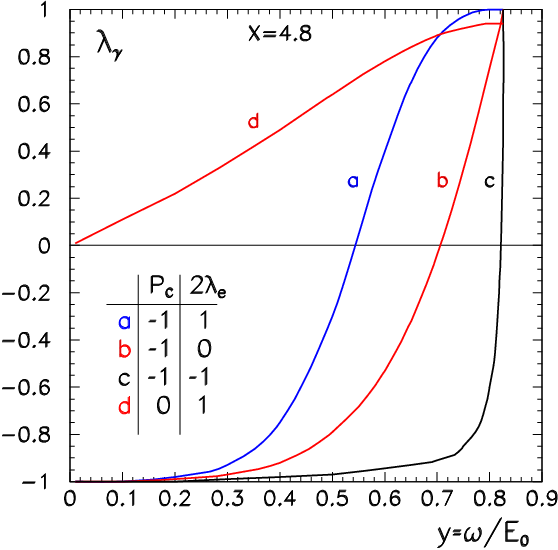
The helicity of the final state photons is given by

The right plot of figure 1 shows the photon helicity for different values of the electron and laser polarisation. $2\lambda_{e}P_{c}=-1$ results in a high and relatively constant polarisation in the high energy peak with a strong variation at lower energies. For $2\lambda_{e}P_{c}=0$ polarising the electron beam is the preferred option.

The photon spectrum in a real collider is more complicated than the one given from pure Compton scattering for two reasons. The laser power is so high that non-linear effects have to be taken into account [6, 7, 8, 9]. They can be parametrised by the parameter

where $\bar{F}$ denotes the field strength of the laser field and $n_{\gamma}$ the corresponding photon density. The non-linear effects modify the photon spectrum in two ways. The effective electron mass increases by a factor $(1+\xi^{2})$ reducing the maximum energy to $\omega_{m}/E_{0}=x/(1+x+\xi^{2})$. At the same time a high energy tail develops due to the simultaneous interaction of one electron with several laser photons. Figure 2 shows the photon energy spectrum for different $\xi^{2}$.

In addition the Compton cross section rises for smaller centre of mass energies. The electrons that have interacted once have thus a high chance to interact a second time giving rise to a much enhanced spectrum at low photon energies.

For the calculation of the luminosity spectrum one has to take into account that lower energy photons are produced at larger angles with respect to the original beam direction so that their luminous spot is larger, reducing the luminosity for low centre of mass energies. To calculate the photon spectrum in a real collider, simulation programs have to be used. In this paper the program CAIN [10] is used which calculates the beam-laser as well as the beam-beam interaction taking non-linearity and beam polarisation effects into account. Figure 3 shows the $\gamma\gamma$ centre of mass energy spectrum and polarisation for the chosen laser parameters and $\sqrt{s}_{\rm ee}=500{\,\mathrm{Ge\kern-1.00006ptV}}$.

A photon collider will be operated with two electron beams instead of an electron and a positron beam for several reasons. Electrons can be polarised to a higher degree than positrons resulting in a more favourable luminosity spectrum. Two electron beams defocus each other in the interaction point generating less beamstrahlung than electron-positron interactions. Electron-electron interactions result in no annihilation events which would be a background for the high energy $\gamma\gamma$ interactions. Since the beamstrahlung for identical beam parameters is smaller at the $\gamma\gamma$ collider than in the $\mathrm{e}^{+}\mathrm{e}^{-}$ case, the beams can be focused stronger resulting in a higher luminosity. Table 1 compares a set of conservative [3] and optimistic [2] parameters with the ones of the $\mathrm{e}^{+}\mathrm{e}^{-}$ collider [3] for a beam energy of 250 GeV. For the optimistic set a third of the $\mathrm{e}^{+}\mathrm{e}^{-}$ luminosity can be obtained in the high energy part of the spectrum. Since the optimistic set results in higher backgrounds it will be used, as a worst case scenario, consistently in this paper. To reach the same physics results with the more conservative set the running time has to be doubled. The total luminosity with the optimistic design is around $\mathcal{L}=10^{35}\mathrm{cm}^{-2}\mathrm{s}^{-1}$, where about 10% are in the interesting high energy region. In the physics studies presented in section 2, it will be assumed that a year of running corresponds to $10^{7}$ seconds at design luminosity.

Figure 4 shows the ${\rm e}\gamma$ luminosity for the $\gamma\gamma$ and for the ${\rm e}\gamma$ collider at $\sqrt{s}_{\rm ee}=500{\,\mathrm{Ge\kern-1.00006ptV}}$, where only one beam is converted and all other parameters are left identical to the $\gamma\gamma$ collider. The ${\rm e}\gamma$ luminosity in the high energy part of the spectrum ($\sqrt{s}_{{\rm e}\gamma}>360{\,\mathrm{Ge\kern-1.00006ptV}}$) is $\mathcal{L}=1.3\cdot 10^{34}\mathrm{cm}^{-2}\mathrm{s}^{-1}$ for the $\gamma\gamma$ collider and $\mathcal{L}=2.4\cdot 10^{34}\mathrm{cm}^{-2}\mathrm{s}^{-1}$ for the ${\rm e}\gamma$ collider.

For parity conserving processes only the total $\gamma\gamma$ and ${\rm e}\gamma$ angular momentum matters. The available states are $|J_{z}|=0,2$ for $\gamma\gamma$ and $|J_{z}|=1/2,3/2$ for ${\rm e}\gamma$¹¹ 1 In the following $J_{z}$ always denotes the total angular momentum for the high energy part of the spectrum.. For studies of CP violation in $\gamma\gamma$ the two $J_{z}=0$ states $\lambda_{\gamma}=(1,1)$ and $\lambda_{\gamma}=(-1,-1)$ give different information, while the two states $J_{z}=\pm 2$ follow from each other by a rotation of the coordinate system. Weak processes violate parity, especially the W couples only to left-handed fermions. For this reason the sign of $J_{z}$ is important for many processes in ${\rm e}\gamma$.

Because of the large disruption of the electron beam in the interaction with the laser the spent beam cannot leave the detector through the hole of the incoming one which is limited by the aperture of the final quadrupole. For this reason a crossing angle is needed. The exact value depends on the size of the final focus quadrupole. This study assumes a value of $\alpha=35\,\mathrm{mrad}$, however with recent quadrupole designs [11] a smaller angle seems possible.

For the simulation of the laser-beam and beam-beam interactions many effects must be taken into account. In the laser-beam interaction non-linear effects are important where the non-linearity varies with space and time and particles can interact several times before they leave the interaction region. In the beam-beam interactions apart from the interesting high-energy events one has to consider coherent effects of a particle from one bunch interacting with the coherent field of the opposing bunch, so called beamstrahlung, and incoherent interactions of single particles from the two bunches. In addition all processes can influence the polarisation of the particles.

All processes are included in the simulation program CAIN [10] which has been used throughout this paper. Where possible CAIN has been checked against GuineaPig [12] and the program of V. Telnov [13]. Reasonable agreement has been found in all cases when a comparison is possible.

For physics studies the beam simulations are not appropriate and fast programs have been developed which generate the interacting beam particles and have been tuned to the beam simulation programs. For the studies presented in this paper the programs CIRCE2 [14], based on a histograming technique, and CompAZ [15], based on analytic parameterisations, have been used.

For the Higgs study a total angular momentum of $J_{z}=0$ is used. In this case the cross sections for the direct continuum $\gamma\gamma\to\rm b\bar{\rm b}$ and $\gamma\gamma\to\rm c\bar{\rm c}$ production, the main background processes, are suppressed by a factor $M_{\rm q}^{2}/s_{\gamma\gamma}$, with $M_{\rm q}$ being the quark mass.

The beam spectra at $\sqrt{s}_{\rm ee}=210{\,\mathrm{Ge\kern-1.15005ptV}}$ are simulated using the CompAZ [15] parameterisation. The response of the detector has been simulated with SIMDET4 [25], a parametric Monte Carlo for the TESLA $\mathrm{e}^{+}\mathrm{e}^{-}$ detector. The only difference between this detector and a Photon Collider detector is the acceptance of the latter at low polar angles which is simulated taking for the Higgs reconstruction only the energy-flow-objects reconstructed with a polar angle above 7⁰.

Signal $\gamma\gamma\to{\rm H}\to{\rm b}\bar{\rm b}$ events corresponding to one year of running are generated using PYTHIA 6.2 [26]. Background processes of the type $\gamma\gamma\to{\rm q}\bar{\rm q}$(g) are generated with the SHERPA [27] generator. A detailed description of the simulation of the background processes with SHERPA can be found in Reference [28].

For $\sqrt{s}_{\rm ee}=210{\,\mathrm{Ge\kern-1.15005ptV}}$ about one pileup event per bunch crossing has to be taken into account. A large fraction of this background is distributed at small angles and it is reduced requiring the cosine of the polar angle of the energy-flow-objects to be below 0.95.

The selection of the events originating from the $\gamma\gamma\to$h$\to{\rm b}\bar{\rm b}$ is described in Reference [29]. Events which contain two or three jets are selected. Jet are reconstructed using the DURHAM [30] algorithm. The invariant mass of the jets has to be consistent with the Higgs mass and two of the jets must be produced by the hadronisation of bottom quarks.

Typical selection variables are: the visible energy of the event; the longitudinal imbalance in the event, the cosine of the thrust angle and the output of the Neural Network [31] for tagging bottom quarks for the fastest two energetic jets in the event.

The reconstructed invariant mass for the selected signal and background processes is shown in the left part of Figure 8 if no pileup is overlaid and in the right part of Figure 8 when on average one pileup event is considered per bunch crossing. To enhance the signal a cut on the invariant mass is tuned such that the statistical significance of the signal over background is maximised. Events in the mass region of 116 GeV $<M_{jj}<132{\,\mathrm{Ge\kern-1.15005ptV}}$ are selected. The number of estimated signal and background events in this window are 3676 and 2317, respectively.

The two photon decay width of the Higgs boson is proportional to the event rates of the Higgs signal. The statistical error of the number of signal events, $\sqrt{N}_{\rm obs}/({\it N}_{\rm obs}-{\it N}_{\rm bkg})$, corresponds to the statistical error of this measurement. Here $N_{\rm obs}$ is the number of observed events, while $N_{\rm bkg}$ is the number of expected background events.

can be obtained. For a Higgs boson with a mass $M_{\rm H}$=120 GeV the product $\Gamma(\rm H\to\gamma\gamma)\times\rm BR(\rm H\to\rm b\bar{\rm b})$ can thus be measured with an accuracy of 2.1$\%$ using an integrated luminosity corresponding to one year of data taking at the TESLA Photon Collider of 80 fb^-1 in the high energy part of the spectrum.

In the ${\rm e}\gamma$ case the “real mode”, where only one electron beam is converted into photons, and the “parasitic mode”, where both beams are converted and the ${\rm e}\gamma$ luminosity of the unconverted electrons is used, have been analysed [34]. Possible backgrounds in the real mode are the $\gamma\gamma$ induced process ${\rm e}\gamma\rightarrow e{\rm q\bar{\rm q}}$ and ${\rm e}\gamma\rightarrow eZ$ where the electron is lost in the forward region. In the parasitic mode in addition $\gamma\gamma\rightarrow{\rm q\bar{\rm q}}$ and $\gamma\gamma\rightarrow\mathrm{W}^{+}\mathrm{W}^{-}$ where one W decays leptonically and the charged lepton is lost, have to be considered.

In the analysis the electron beam always has been assumed to be dominantly left-handed and the ${\rm e}\gamma$ angular momentum is set to $|J_{z}|=3/2$, which is the more sensitive configuration because of the missing s-channel.

In a first step of the analysis pileup tracks are rejected. Tracks are rejected if their $z$-impact parameter is inconsistent with the primary vertex. In addition tracks are rejected if they are far away from the reconstructed W-axis where the cut is stronger if the tracks are in the forward region. Figure 10 shows the reconstructed W mass and energy distribution using all tracks, the tracks that pass the impact parameter cut and the tracks that pass in addition the angle cuts. The large tails get reduced significantly by the cuts for the price of a worse mass resolution. In a second step events are selected by a cut on the reconstructed mass and energy of the W. These cuts result in an efficiency of 73% (66%) with a purity of 64% (49%) in the real (parasitic) mode. The background is extremely forward peaked and an additional cut of $\theta_{W}>5^{\circ}$ results in a purity of 95% (72%) basically without a loss in efficiency.

The events are fitted using a Monte Carlo reweighting technique where Whizard [36] is used as a generator. In the fit the W production angle, the two decay angles and the energy are used. In addition to the triple gauge couplings a free normalisation constant is fitted, where the normalisation is constrained to unity with an assumed error on the efficiency and luminosity determination.

Table 2 summarises the results for different fit assumptions assuming one year of running. The precision on $\kappa_{\gamma}$ depends mainly in the precision on the total cross section and thus on the assumed normalisation error. $\lambda_{\gamma}$ has only little sensitivity to the normalisation but is more sensitive to pileup and background. The correlation between $\Delta\kappa_{\gamma}$ and $\Delta\lambda_{\gamma}$ is negligible in all cases.

Several sources of systematic errors have been considered. Assuming $\Delta\mathcal{L}/\mathcal{L}=0.1\%$ the beam polarisation needs to be known to 0.1% in order that $\Delta\kappa_{\gamma}$ is not dominated by this error. At the same time the background has to be known to a precision of better than 3% in the real mode and 1% in the parasitic mode. $\lambda_{\gamma}$ is basically not sensitive to both variations. Both coupling constants are not sensitive to realistic variations in the luminosity spectrum.

A similar analysis has been performed for $\gamma\gamma\rightarrow\mathrm{W}^{+}\mathrm{W}^{-}$ using both angular momentum states $|J_{z}|=0,2$ [35]. The only relevant background for this channel is the process $\gamma\gamma\rightarrow{\rm q\bar{\rm q}}$ where four jets are produced from gluon radiation. Since there are always two W-bosons in the event, typically at low angles, angular cuts are not effective against pileup, which can thus only be rejected by the impact parameter cut. Events are selected by cuts on the reconstructed invariant mass of the W-bosons and the angle between the two jets belonging to one W in the centre of mass frame of the event. With these cuts an efficiency of $\sim 50\%$ and a purity of $\sim 80\%$ has been achieved for both $J_{z}$ states.

The data have also been fitted with a Monte Carlo reweighting technique. In this case the fit has been done in six dimensions, the W-production angle, two decay angles per W and the WW centre of mass energy. Again the two anomalous couplings have been fitted together with a free but constrained normalisation factor. Table 3 summarises the results for the two angular momentum states for one year of running. Like in $e\gamma$ the sensitivity to $\kappa_{\gamma}$ is determined by the cross section measurement while $\lambda_{\gamma}$ is given by the shape of the events. Consequently $\lambda_{\gamma}$ suffers more from the presence of pileup and background. $\lambda_{\gamma}$ is determined better from $|J_{z}|=2$ while for the same luminosity error $J_{z}=0$ is more sensitive to $\kappa_{\gamma}$. However the luminosity can be determined much more precise in $|J_{z}|=2$ so that this mode is the better one for both coupling constants.

Figure 11 compares the precision of the fits to $\kappa_{\gamma}$ and $\lambda_{\gamma}$ for the different machines. For $\mathrm{e}^{+}\mathrm{e}^{-}$ the results for the 5-parameter fit to $g_{Z},\kappa_{\gamma},\kappa_{Z},\lambda_{\gamma},\lambda_{Z}$ are shown. For $\kappa_{\gamma}$ $\mathrm{e}^{+}\mathrm{e}^{-}$ is clearly superior to $\gamma\gamma$ and ${\rm e}\gamma$. For $\lambda_{\gamma}$ the photon collider is better in both modes, however generator studies indicate that LHC could reach a similar accuracy.

In most models the $\tilde{\mu}_{\rm R}$ decays only into $\mu{\tilde{\chi}}^{0}_{1}$ so that for $\tilde{\mu}_{\rm R}$-pair production probably no information on Supersymmetry breaking parameters can be obtained. Nevertheless this process has been simulated inside SPS1a [40]. The process is mainly characterised by an acoplanar muon pair in the detector. Below the $\tilde{\mu}_{\rm L}$ production threshold the main background is W-pair production. The signal can be selected with an efficiency of 85% and a purity of 59% resulting in a precision on the cross section measurement of 1.6% in a month of running ($100\,\,\,{\rm fb}^{-1}$) with $J_{z}=0$. This cross section precision can also be interpreted as a 0.8% precision of the branching ratio $BR(\tilde{\mu}_{\rm R}\rightarrow\mu{\tilde{\chi}}^{0}_{1})$ where it has to be assumed that possible other $\tilde{\mu}_{\rm R}$ decays don’t give any background to the selected channel.

In the SPS1a scenario the study of $\tilde{\mu}_{\rm L}$ decays is much more interesting, since three decay channels are open $\tilde{\mu}_{\rm L}\rightarrow\mu{\tilde{\chi}}^{0}_{1}$ (55%), $\tilde{\mu}_{\rm L}\rightarrow\mu{\tilde{\chi}}^{0}_{2}$ (17%) and $\tilde{\mu}_{\rm L}\rightarrow\nu_{\mu}{\tilde{\chi}}^{\pm}_{1}$ (28%). $\tilde{\mu}_{\rm L}$ pair production has been simulated at $\sqrt{s}_{\rm ee}=600{\,\mathrm{Ge\kern-1.15005ptV}}$ with $J_{z}=0$ where one expects $3\cdot 10^{4}$ events in one year of running [40]. Figure 12 shows the muon momentum distribution from $\tilde{\mu}_{\rm L}$ decays together with the expected background. For the signal one can see three distinct regions. At high momenta there are only muons from the $\tilde{\mu}_{\rm L}\rightarrow\mu{\tilde{\chi}}^{0}_{1}$ decay, the muons at medium momenta are from the $\tilde{\mu}_{\rm L}\rightarrow\mu{\tilde{\chi}}^{0}_{2}$ decay and the ones at low momenta are from ${\tilde{\chi}}^{0}_{2}$ decays.

Selecting the high momentum region one can with similar cuts as for the $\tilde{\mu}_{\rm R}$ analysis measure the cross section $\gamma\gamma\rightarrow\tilde{\mu}_{\rm L}++\tilde{\mu}_{\rm L}^{-}\rightarrow\mu^{+}{\tilde{\chi}}^{0}_{1}\mu^{-}{\tilde{\chi}}^{0}_{1}$ with a precision of around 2% and the corresponding branching ratio ${\rm BR}(\tilde{\mu}_{\rm L}\rightarrow\mu{\tilde{\chi}}^{0}_{1})$ with a precision of around 1%. This branching ratio should be sensitive to the mixing angles in the chargino and neutralino sector.

A chargino can decay either into a W and a neutralino or, if kinematically allowed, into a slepton and the corresponding lepton³³ 3 Other decays like decays into virtual squarks are usually suppressed. The flavour composition of the leptons is non-trivial and depends on the SUSY-breaking parameters. Within SPS1a the ${\tilde{\chi}}^{\pm}_{1}$ decays almost exclusively into $\tilde{{\tau}_{1}}\nu_{\tau}$, so that no meaningful branching ratio measurement is possible. Therefore for a simulation study $m_{0}$ has been changed to $130{\,\mathrm{Ge\kern-1.15005ptV}}$ and $\tan\beta$ to 9. With these parameters the ${\tilde{\chi}}^{\pm}_{1}$ decays in 26% of the cases into $W{\tilde{\chi}}^{0}_{1}$ and in 73% into $\tilde{{\tau}_{1}}\nu_{\tau}$. The process $\gamma\gamma\rightarrow{\tilde{\chi}}^{+}_{1}{\tilde{\chi}}^{-}_{1}$ has been simulated with both charginos decaying into ${\rm W}{\tilde{\chi}}^{0}_{1}$ and the W decaying hadronically. Details of the analysis can be found in [41]. Assuming that the production cross section is known the event rate is proportional to ${\rm BR}({\tilde{\chi}}^{\pm}_{1}\rightarrow{\rm W}{\tilde{\chi}}^{0}_{1})^{2}$.

Because of the huge WW background an efficiency of 24% and a purity of 11% is possible at $\sqrt{s}_{\rm ee}=600{\,\mathrm{Ge\kern-1.15005ptV}}$, leading to a relative branching ratio error of 3.5%. To test the usefulness of this measurement it has been injected into the fit of the low energy SUSY breaking parameters with Fittino using the masses and cross sections from the LC/LHC study [42]. Due to the ${\tilde{\chi}}^{\pm}_{1}$ branching ratio measurements the precision on $\tan\beta$ and on the $\tilde{\tau}$ mixing parameter improve by a factor two to three. However up to now no decay related observables from $\mathrm{e}^{+}\mathrm{e}^{-}$ are used in the fit.

If the mass difference $\tilde{{\rm e}}_{\rm R}{\tilde{\chi}}^{0}_{1}$ is large it is possible that the reaction $\mathrm{e}^{+}\mathrm{e}^{-}\rightarrow\tilde{{\rm e}}_{\rm R}^{+}\tilde{{\rm e}}_{\rm R}^{-}$ is not accessible while ${\rm e}\gamma\rightarrow\tilde{{\rm e}}_{\rm R}{\tilde{\chi}}^{0}_{1}$ can be seen at the same ${\rm e}^{-}{\rm e}^{-}$ centre of mass energy. In mSUGRA this happens e.g. if $m_{0}$ and $m_{1/2}$ are of approximately the same size. If this happens in mSUGRA the chargino and neutralino sector would be accessible in $\mathrm{e}^{+}\mathrm{e}^{-}$ via $\mathrm{e}^{+}\mathrm{e}^{-}\rightarrow{\tilde{\chi}}^{0}_{1}{\tilde{\chi}}^{0}_{2},\,{\tilde{\chi}}^{0}_{2}{\tilde{\chi}}^{0}_{2},\,{\tilde{\chi}}^{+}_{1}{\tilde{\chi}}^{-}_{1}$ so that $m_{1/2}$ could be measured already there while $m_{0}$ can only be obtained from the $e\gamma$ mode. Without gauge unification it is also possible to adjust the parameters in a way that no visible SUSY signal is present in $\mathrm{e}^{+}\mathrm{e}^{-}$.

In most models the $\tilde{{\rm e}}_{\rm R}$ decays dominantly into ${\rm e}{\tilde{\chi}}^{0}_{1}$ so that if R-parity is conserved the experimental signal is a single electron in the detector. There are two irreducible background channels: ${\rm e}\gamma\rightarrow{\rm W}\nu$ with ${\rm W}\rightarrow{\rm e}\nu$ and ${\rm W}\rightarrow\tau\nu\rightarrow{\rm e}3\nu$ and ${\rm e}\gamma\rightarrow{\rm eZ}\rightarrow{\rm e}\nu\bar{\nu}$. In most cases the lightest sfermion is the partner of the right-handed electron, so that the signal is enhanced using right-handed electron beams. This polarisation suppresses simultaneously the W-background which is present for left-handed electrons only. Also the Z-background is reduced slightly in this case.

Signal and background have been simulated using SHERPA [27] where the following SUSY parameters have been used:

resulting in

with the $\tilde{{\rm e}}_{\rm R}$ decaying almost exclusively into ${\rm e}{\tilde{\chi}}^{0}_{1}$ [43]. With cuts in the electron energy and polar angle an efficiency of $\varepsilon=71\%$ and a purity $p=63\%$ can be reached allowing a 1% cross section measurement in one year of running. As shown in [17] the selectron and neutralino mass can be obtained from the two endpoints of the electron energy spectrum in case of monoenergetic beams. For the simulated parameter set the neutralino mass can be measured in $\mathrm{e}^{+}\mathrm{e}^{-}$ running, so that one endpoint is sufficient to obtain the selectron mass. Because of the sharp upper edge of the photon energy spectrum the lower endpoint is approximately preserved. The upper edge gets distorted by the dependence of the $\tilde{{\rm e}}_{\rm R}$-energy from its polar angle but can be reconstructed from the electron transverse momentum. It has been estimated that from the lower endpoint the selectron mass can be measured with a precision of 0.5%. The precision from the upper endpoint is significantly worse.

Inside an optical ring resonator the circulating electric field directly after the input coupling mirror $M_{c}$ is given by a superposition of the transmitted incoming electric field and a scaled replica of the circulating field that emerged from this coupling mirror at the previous round-trip. On resonance the power enhancement factor $A_{q}$ describes a monotonous increase of power after the cavity has been filled with $q$ pulses:

$R_{c}$ represents the intensity reflectivity of the coupling mirror and $V$ the power loss factor for one round-trip.

If the reflectivity of the coupling mirror equals the loss factor $V$ of the cavity, the maximum possible steady-state power enhancement factor of $A_{\infty}=1/(1-V)$ is obtained and all light is absorbed by the resonant cavity. This is known as impedance matching.

On resonance no power will be reflected from an impedance matched cavity in steady state. The reflected power can be used as an indicator for the alignment of the cavity in an automated control system.

To maintain a sufficiently high photon density and hence a high conversion factor, the laser pulse must be focused at the Compton conversion point (CP). When operated at the inevitable high power level optical windows within the cavity would imply the risk of distortion of the circulating optical picosecond-pulse as a result of the non-vanishing B-integral [52, 53]. The Compton-interaction requires therefore operation of the cavity in the vacuum of the accelerator.

Due to space limitations and to avoid vibrations any component of the optical cavity should preferably be positioned outside the environment of the particle detector, a few metres away from the laser focus. As a consequence of the required tight optical focus and the large distance the cross section of the laser beam will increase to more than half a metre at the location of the final focusing mirror.

Compton conversion at each of the counter-propagating electron beams requires two ring cavities as exemplified by Fig. 14. They are interlaced without mutual interference.

Their optical paths are enclosed within the associated optical beam pipes which are needed to maintain the vacuum. For details see [51]. The focusing is accomplished by means of a mirror telescope (inverted beam expander) and a second, identical telescope is used for re-collimation.

The focal spot size at the CP and the influence of the finite diameter of the mirrors were calculated numerically [51]. Total correction of the aberrations introduced by the telescope mirrors was thereby assumed. That necessitates e.g. the use of off-axis parabolic mirrors. The diameter of the final focusing concave mirrors (denoted by the subscript ”cc” in related symbols) determines the minimal collision angle $\alpha_{L}$ between the laser and the electron beam. It should be kept small for high yield of photons. The major effect in reducing the size of the mirrors is a diffractive broadening of the focal spot size. The increased loss due to radiative energy that spills over the boundaries of the mirrors turned out to be much smaller. Figure 15 shows the broadening of the focal spot due to the finite size of the focusing mirror as a function of the radius of this mirror.

In order to calculate the laser-electron crossing angle $\alpha_{L}$ and to specify the beam waist $\widetilde{w_{0}}$ for finite mirror size, diffraction broadening has to be taken into account. To optimise the yield of photons, the crossing angle $\alpha_{L}$, the mirror diameter $2\,a_{cc}$, the waist size $\widetilde{w_{0}}$, the laser pulse energy $E_{pulse}$, as well as the laser pulse duration $\tau_{pulse}$ are all interdependent parameters. Their respective values were determined by a numerical optimisation process using the program CAIN [10] to calculate the yield. CAIN assumes that charged particles interact with a Gaussian optical beam. The centre-of-mass energy was set to 500 GeV. The aperture $2\,a_{cc}$ of the final focusing concave mirrors $M_{4}$, $M_{5}$ at distance $L_{image}$ from the conversion point CP in Fig. 16 sets an upper limit for the opening angle $\theta_{cc}$ of the laser cone that emerges from the beam waist:

Replacing $L_{image}$ by the far field divergence angle $\theta$ originating from a Gaussian beam waist $w_{0}$ results in the latter equation. $w_{cc,G}$ represents the beam radius on each of the concave mirrors. If the electron beams cross each other in the horizontal ($x-z$) plane, the laser beams should run in the vertical ($y-z$) plane. To allow for an opening angle of the outgoing beampipe of 14 mrad and the finite size of the focusing quadrupole, it is assumed that the lower edge of the laser beampipe stays away from the horizontal plane by 17 mrad. If the quadrupole can be smaller a lower offset angle is possible allowing for a slightly smaller laser power or higher luminosity. The projection of the different pipes in the $x-y$ plane at the front face of the final quadrupole is shown in figure 17.

The crossing angle $\alpha_{L}$ is thus expressed as

This relation was encoded into CAIN via the optical Rayleigh length $z_{R}=\pi\,w_{0}^{2}/(M^{2}\lambda$) and the relation $\theta=w_{0}/z_{R}$. The beam quality factor $M^{2}$ equals $1$ only for Gaussian beams [54]. For more general beams holds $M^{2}$ $>$ 1, and the waist can be expressed as $\widetilde{w_{0}}$ = $M^{2}\,w_{0}$. It turned out that near the focus the diffraction broadened beam is well approximated when substituting $M^{2}$ by $\gamma$, and hence $\widetilde{w_{0}}$ = $\gamma\,w_{0}$ has been used instead of the Gaussian beam waist $w_{0}$. Fig. 18 shows the resulting luminosity as a function of the crossing angle $\alpha_{L}$ for different mirror sizes $a_{cc}/w_{cc,G}$ and a laser pulse duration of $\tau_{L}=3.5$ ps FWHM ($\sigma$ = 1.5 ps). In the examined range the luminosity rises with decreasing diameter of the mirrors. A value of $a_{cc}/w_{cc,G}=0.75$ is therefore selected. An acceptable crossing angle is then $\alpha_{L}\,\approx\,55$ mrad. This corresponds to a Rayleigh length $z_{R}$ $\approx$ 0.63 mm, a diffraction broadened beam waist of $\widetilde{w_{0}}$ $\approx$ 14.3 $\mu$m⁴⁴ 4 $\widetilde{w_{0}}$ is given in the $1/e^{2}$ convention, designating the radius that is defined by a drop of the intensity to $1/e^{2}$ $\approx$ 13.5 % of its maximum value at the beam centre. Given in Gaussian $\sigma$ its value is a factor two smaller. and a nominal Gaussian waist of $w_{0}$ $\approx$ 6.5 $\mu$m.

The behaviour at small crossing angle has been verified by a program calculating the overlap integral of the electron beam and the laser and can be understood as follows. Because of the offset the length of the overlap region increases with $\sqrt{z_{R}}$, i.e. smaller crossing angles. On the other hand the beam widens in two directions so that the photon density decreases with $1/z_{R}$ resulting in a $1/\sqrt{z_{R}}$ decrease of the conversion probability. Without the offset the length increases in principle with $z_{R}$, however the length of the overlap region is limited by the duration of the laser spot. At large crossing angle the overlap integral continues to increase. However the conversion probability is limited to one and because of the increasing non-linearity the spectrum is shifted to lower energies which are not considered in our definition of the luminosity.

A total luminosity⁵⁵ 5 Here $z_{max}$ is defined as $z_{max}=x/(x+1+\xi^{2})$ consistent with the definition in [2]. of ${\mathcal{L}}(z>0.8z_{max})=1.1\cdot 10^{34}\,{\rm cm^{-2}s^{-1}}$ can be achieved for these parameters with a pulse energy of 9 J [55]. A non-linearity parameter $\xi^{2}=0.3$ can be maintained in accordance with reference [2], however the required laser power is 80% larger. In proportion to the laser pulse energy the required average laser power has also gone up to $9\,{\rm J}\times 2820\times 5\,{\rm Hz}\approx 130\,{\rm kW}$. All resulting parameters for the Compton interaction zone of a $\gamma\gamma$-collider based on 250 GeV electron beams are compiled in Tab. 5.

According to the results obtained in [51] all mirrors could have a diameter of about 120 cm. In this case cutoff occurs at approximately 75 % of the hypothetical Gaussian beam radius $(1/e^{2})$ at the final focusing mirror which represents the dominant aperture at which diffraction will occur.

An estimated fractional power loss due to diffraction of roughly $LF_{\rm diff}\geq 0.9998$ per round trip and a reflectivity of between $R_{HR}$ = 99.99 % and 99.95 % for presently available standard mirror coatings would permit a steady-state impedance matched power enhancement between 1100 and 270, for otherwise perfect conditions⁶⁶ 6 Such reflectivities are currently readily available only for mirror substrates of a few cm diameter. This is not limited due to any principles of physics. For optical gravitational wave detection similar mirrors of about 30 cm diameter have already been manufactured. This topic certainly requires further technological effort.. The enhancement becomes the more sensitive against any impedance mismatch, the larger $A_{\infty}$ is.

The optical energy fluence of $\approx$ 13 J/cm² is expected to be well below the damage threshold of mirror substrates and coatings. However, no data for trains of ps-pulses separated on nano- to microsecond time scales which accumulate to the stated fluence exist. For a final judgement an experimental study with a representative of the ILC bunch structure would be required.

Any misalignment of a mirror position and orientation generally results in displacement and broadening of the intra-cavity beam waist. According to our calculations, the displacement of the beam waist remains smaller than the Rayleigh length, i.e. the depth of the focus. This shift of the beam waist is hence negligible.

Transversely the laser beam has to collide with the electron beam which requires a precision of $<10\,\mu\mathrm{m}$. Feedback algorithms for this need to be developed. They could use the power of the high energy photon beam as well as the optical radiation leaking through one of the focusing mirrors around the Compton interaction point

Maintaining the power enhancement factor e.g. above 90 % of its optimum value $A_{\infty}$ demands sub-nm precision for controlling the circumference. Technical solutions for such a precise length stabilisation are well-known [56]. Even more stringent restrictions are common in interferometrical detection of gravitational waves. For the latter case control loops for automatic alignment have been developed. Despite the different operation modes, the use of bursts of optical ps-pulses for the $\gamma\gamma$ collider and continuous-wave (cw) laser radiation in optical interferometers for gravitational waves, the cavity for the $\gamma\gamma$-collider should benefit from that knowledge. In addition, adaptive optics appears to be essential for operation of such a cavity for the photon collider [51].