Parametric instabilities in magnetized multicomponent plasmas
Abstract
This paper investigates the excitation of various natural modes in a magnetized bi-ion or dusty plasma. The excitation is provided by parametrically pumping the magnetic field. Here two ion-like species are allowed to be fully mobile. This generalizes our previous work where the second heavy species was taken to be stationary. Their collection of charge from the background neutral plasma modifies the dispersion properties of the pump and excited waves. The introduction of an extra mobile species adds extra modes to both these types of waves. We firstly investigate the pump wave in detail, in the case where the background magnetic field is perpendicular to the direction of propagation of the pump wave. Then we derive the dispersion equation relating the pump to the excited wave for modes propagating parallel to the background magnetic field. It is found that there are a total of twelve resonant interactions allowed, whose various growth rates are calculated and discussed.
pacs
52.35.Bj, 52.35.Mw, 52.30.Ex, 52.25.VyI Introduction
The basic natural modes of magnetized plasmas such as those that occur in molecular clouds, cometary plasmas and stellar atmospheres are of great interest. When the frequencies are low then a class of linear waves, referred to collectively as Alfvén waves, are known to exist and are of importance to the understanding of many basic plasma phenomena Movspitz; Movpil. The linear approximation to these waves breaks down at large amplitudes where nonlinear effects become important in their propagation. One such large amplitude wave is a magnetoacoustic wave, which modifies the background magnetic field in an oscillatory fashion, and so can be considered as a pump wave that drives other waves nonlinearly. Such large-amplitude pump waves may occur in conditions such as seen in solar and space plasmas. For example, solar shock waves can set up large amplitude standing magnetoacoustic waves in coronal loops or magnetic flux tubes MovSakai1; MovSakai2; Movdurrant.
By considering perturbations of this large amplitude pump, we can investigate the possibility of exciting natural modes of the system, such as Alfvén waves, due to a resonant interaction between the pump wave and the natural waves. In the single ion species case this basic phenomenon was predicted by MovMont; MovVahal, and subsequently pursued by several authors MovCramer; MovMjol; MovMoral. For a pump magnetic field parallel to the background magnetic field in a single ion species plasma, the excited waves are Alfvén waves travelling in opposite directions along the magnetic field MovMont; MovVahal. If ion-cyclotron effects are included, the excited waves are the fast and slow (ion–cyclotron) Alfvén waves travelling in opposite directions MovCramer. More general behavior is allowed in the case where the excited waves are permitted to travel obliquely to the magnetic field MovCramer76.
The parametric excitation of waves in a dusty magnetized plasma has been investigated in Ref. MovHertz, but in the approximation where the dust is taken to be immobile. In that case the oppositely travelling pair of waves are modified, with the presence of a cutoff frequency in the fast Alfvén wave. Furthermore, an interaction between a pair of fast waves or a pair of slow waves was found to exist. The corresponding growth rates of the slow-fast and fast-fast pairs were maximized as a function of the dust concentration.
Many space and laboratory plasmas are multicomponent, i.e., contain multiple ion species. It is therefore of great interest to investigate the effects of the additional species on the linear and nonlinear properties of the waves in the plasma. For instance, it is often the case that in the presence of an additional ion component an extra mode is excited, or forbidden regions of frequency are introduced. One area of study of multi-ion plasmas is the bi-ion plasma. The inclusion of one extra ion species often captures the basic information of several extra species. The bi-ion plasma has particular importance in plasma fusion, laboratory plasmas and in astrophysical environments, with the secondary ion usually positively charged.
A dusty plasma adds another level of interest to the topic of multicomponent plasmas, due to the dust properties. Dust is an additional impurity of large mass and often of negative charge. Under the simplest approximation, all the dust grains may be considered to have the same mass and equilibrium charge, and so are equivalent to a second ion species. This is the case considered in this paper. It is known that the inclusion of dust in a plasma may introduce cutoff frequencies into the basic Alfvén waves, and introduce a low frequency mode, whose nature is different from that in a bi-ion plasma due to the dust grain’s extremely high mass MovVlad; MovCrambk. Qualitative differences to the bi-ion case arise when charge perturbations of the grains are included, leading to an additional damping mechanism Movvlprop, or when a spectrum of dust grain sizes and charges is allowed for Movspectrum. Dust is found, in varying amounts, in many astrophysical and space environments such as molecular clouds and the rings of Saturn. Dusty plasmas have also been studied closely experimentally, since the heavy grain mass introduces low frequency effects that may be studied in real time.
An immediate consequence of the presence of an additional ion species is its modification of the background free-electron number density. This influences the propagation of plasma and electromagnetic waves Movvlprop; Movvlscat; Movcrvl. If in the case of a dusty plasma we fix the grain charge, then the grain becomes entirely defined in terms of its mass and charge, and as such acts just like another ion in the plasma (albeit of negative charge). The state of charge neutrality may be written as:
| (1) |
Here is the number density of plasma electrons (with the charge ), and the two ion species (of signed charge and ), respectively. For laboratory dusty plasmas, the grain charge is negative (i.e., ) and large (), so that an appreciable proportion of the negative charge in the plasma may reside on the dust particles. For astrophysical dusty plasmas, may only be of the order of unity, which is often the case for a canonical bi-ion plasma. In environments such as the interstellar medium, where the dust grain is in an electron-proton plasma with little ultra-violet radiation present, the dust grains acquire a negative charge. On the other hand, exposure to ultraviolet light from nearby stars can cause ionization of the grains, leaving a residual positive charge.
In this paper, we investigate the propagation of plane hydromagnetic waves (Alfvén waves and magnetoacoustic waves modified by the presence of a secondary ion or dust species in a bi-ion plasma), propagating parallel to the pumped magnetic field of a large amplitude magnetoacoustic wave. We generalize Ref. MovHertz where the second heavy space was assumed immobile, to the case where both ions are fully mobile. A further generalization is the inclusion of pressure. The background magnetic field and plasma density are taken to be uniform, at frequencies well below the electron plasma and cyclotron frequencies. First, we find the dispersion equation of the pump wave, and then concentrate on pump waves of large wavelength. We then obtain a coupled pair of equations of motion governing the perturbed plasma. Resonant interactions are sought, and growth rates of the waves parametrically excited by the pump are calculated and discussed.
II Multifluid Model
The most general set of equations used to describe two mobile ion-like species, plus electrons, is a three-fluid model. In this picture we employ three momentum equations for the electrons and the two ion species, where we include both the ions’ inertia terms, while ignoring the electron inertia. This is valid if the frequencies of interest are well below the electron cyclotron frequency. In addition we use Maxwell’s equations and two mass continuity equations for each of the ion species, ignoring Maxwell’s displacement current.
The primary species (assumed positively charged) shall be denoted with a “1” subscript, and the secondary species (either positively or negatively charged) shall be denoted with a “2” subscript. In this notation we may write the current density as
| (2) |
where the two ion species and electrons have velocities denoted by , , and , respectively. We employ the parameters and , which measure the distribution of charge in the plasma amongst the ions. Employing the total charge neutrality condition, given in Eq. (1), we may write this as
| (3) |
in terms of these parameters. Note that in the limit of a single (primary) ion species, we have and .
Ignoring collisions, but including the effects of pressure, the starting equations for the velocities, electric and magnetic fields and each number density are the momentum equations, the two ion continuity equations, and Ampere’s law neglecting the displacement current:
| (4) | |||||
| (5) | |||||
| (6) | |||||
| (7) | |||||
| (8) | |||||
| (9) |
Here, are the two heavy species and electron pressures, and are the heavy masses. The magnetic field includes the background magnetic field .
Finally, by assuming either an isothermal or an adiabatic equation of state, we have
| (10) |
for each species, where are the individual sound speeds. Though it is not imperative, we shall assume isothermal changes, which permits us to write down in terms of the plasma temperatures, i.e., is the square of each thermal speed, where is each temperature and is Boltzmann’s constant.
At this point we choose to eliminate the electron variables from Eqs. (4)–(9), and use Faraday’s law to eliminate the electric field . There are then two choices for the way to proceed. We can add and subtract the momentum equations and deal with a total fluid velocity and the current density . Instead we shall employ the most direct method, which is to deal with the ion velocities and separately, since our equations will exhibit the most symmetry this way. By employing the charge neutrality condition to all orders, the following system of nonlinear partial differential equations is found:
| (11) | |||||
| (12) | |||||
| (13) | |||||
| (14) | |||||
| (15) | |||||
In Eqs. (11)–(15) are the densities of each massive component of the plasma and are the corresponding (signed) cyclotron frequencies, with . Also and are pseudo-squared thermal speeds associated with the electron pressure (if we allow to be imaginary). The presence of both and in both equations of motion, is a consequence of the elimination of the electron variables from the equations. To be more explicit, the electron density fluctuations generate fluctuations in both the ion densities through the charge neutrality condition, which produces this coupling in the momentum equations. The second term on the right hand side of Eq. (13) is the Hall term; it is important when the wave frequency is comparable to either of the cyclotron frequencies. Also, we see that the two species are strongly coupled through the momentum equations, via the third term on the right hand side in each. This is an additional Hall-type term associated with the relative motion of the two species. Note Eqs. (11)–(14) reduce, in the case of a single species plasma (, assuming local charge neutrality is maintained), to the equations used in Ref. Movmio; Movmjolh76; Movspsh; Movmjwy86; Movovendon where nonlinear Alfvén waves were investigated. They are then known as the (collisionless) Hall-MHD (magnetohydrodynamics) equations.
The neglect of the displacement current in Maxwell’s equation is justified when the electron current is much greater than the displacement current, which leads to the conditions
| (16) |
where is the wave frequency and are the Alfvén speeds associated with each ion. The charge neutrality condition implies that the wave frequencies are restricted to the regime , which may be restated as
| (17) |
There exists a wide range of physical environments for which all of the above mentioned conditions are met.
III Magnetoacoustic Pump Wave
Suppose there is a constant background magnetic field in the -direction, given by . We now periodically pump the field, with a periodic modulation:
| (18) |
where is the pump frequency. Here is a constant dimensionless quantity which determines the amplitude of the pump. More precisely, is an expansion parameter, which permits us to keep track of our terms, by matching powers of . The parameter on the other hand is a dimensionless quantity that we include to capture any necessary frequency information, i.e., , such that the average of over is . By specifying a particular choice of normalization condition, we may solve for . We later in fact impose the condition that the energy density in the pump system is a constant over , and calculate the resulting . Since we are interested in a large amplitude pump wave, will typically be .
However, since this field has no spatial dependence, it does not satisfy our wave equations. Hence this is an approximation to a wave with a large wavelength. We must therefore modify the pump with an envelope of some wavelength. Since the pump wave magnetic field points in the -direction, the wavevector should point perpendicular to this to satisfy . For a planar geometry plasma, we choose the axes such that the wave varies in the -direction, with wavenumber . By denoting the pump magnetic field (and all subsequent pump fields) with a “0” superscript, we have
| (19) |
In a cylindrical plasma, with denoting the radial distance from the cylindrical axis, we have
| (20) |
where is the 0th order Bessel function of the first kind. Note that in Eqs. (19) and (20).
In the absence of a wave, we shall suppose that the plasma is stationary, with ion densities and charge ratios of . The effect of pumping will be to modify the velocity, density and charge imbalance to order , so that
| (21) | |||||
| (22) | |||||
| (23) |
These quantities define the pump wave, and we now proceed to solve the equations (11)–(15) to order (i.e., the linear solution).
By inspecting the form of the magnetic field in Eq. (19) [or (20)], and Eqs. (14) and (15), we note that the velocity cannot have a -component. Hence, the velocities of the ion species must be of the form
| (24) |
for planar waves. From the resulting pair of equations we ascertain the form of each velocity component and density:
| (25) | |||||
| (26) | |||||
| (27) |
where and are amplitudes independent of space and time, to be determined. Then, from the continuity equations, we have
| (28) |
For the cylindrical plasma case, we make the substitutions: , , and , where is the azimuthal angle and is the 1st order Bessel function of the first kind. Then it is found that all the relationships (24)–(28) still hold. It follows that the modes in the planar and cylindrical plasmas satisfy the same dispersion equation.
Upon substitution of Eqs. (25)–(28) into Eqs. (11)–(15), written to first order in , the following dispersion equation of the pump wave is obtained:
| (29) |
Here, we have defined
| (30) | |||||
| (31) | |||||
| (32) | |||||
| (33) | |||||
where is a hybrid cutoff frequency as . Also we have introduced , , and which allow us to specify the cold/warm plasma regimes, with and related through: . Note that as (i.e., a single species) we are left with the nondispersive relation
| (34) |
where is the combined sound speed in this limit. This is the familiar fast magnetoacoustic wave characteristic for . However, in the presence of a secondary ion species the fast magnetoacoustic wave gains an additional mode and the relationship is dispersive, see Fig. 1.


It is easy to show that the parameters and are always positive, while for the cold plasma and is positive if any of are nonzero. Although Fig. 1 is for a plasma in which the secondary ion species is positive, the same basic qualitative features are present when the second ion species is negative. For the warm plasma the effect of the term in the dispersion relation is to cause the lower branch to increase without bound as , as indicated in Fig. 1(a). Physically, it can be thought of as the fast magnetoacoustic mode being converted into an acoustic mode for large due to the inclusion of pressure. However, if the plasma is cold (i.e., ) then the lower branch experiences a resonance as , as indicated in Fig. 1(b). In this limit becomes the square of a resonance frequency, given by
| (35) |
which gives rise to a forbidden frequency region between and , since whenever .
The ratio of the -velocity amplitudes to the magnetic field parameter are of particular importance to our later discussion, so we briefly discuss them here. In terms of the frequency and wavenumber, we find,
| (36) |
where
| (37) |
Finally, to complete the set of pump quantities, we find that the velocity in the -direction is given by
| (38) |
with given similarly. This is quite different to the single ion species case, where .
The behavior of is dramatically altered by the choice of branch from the dispersion relation; see Fig. 2, where for brevity we plot only.
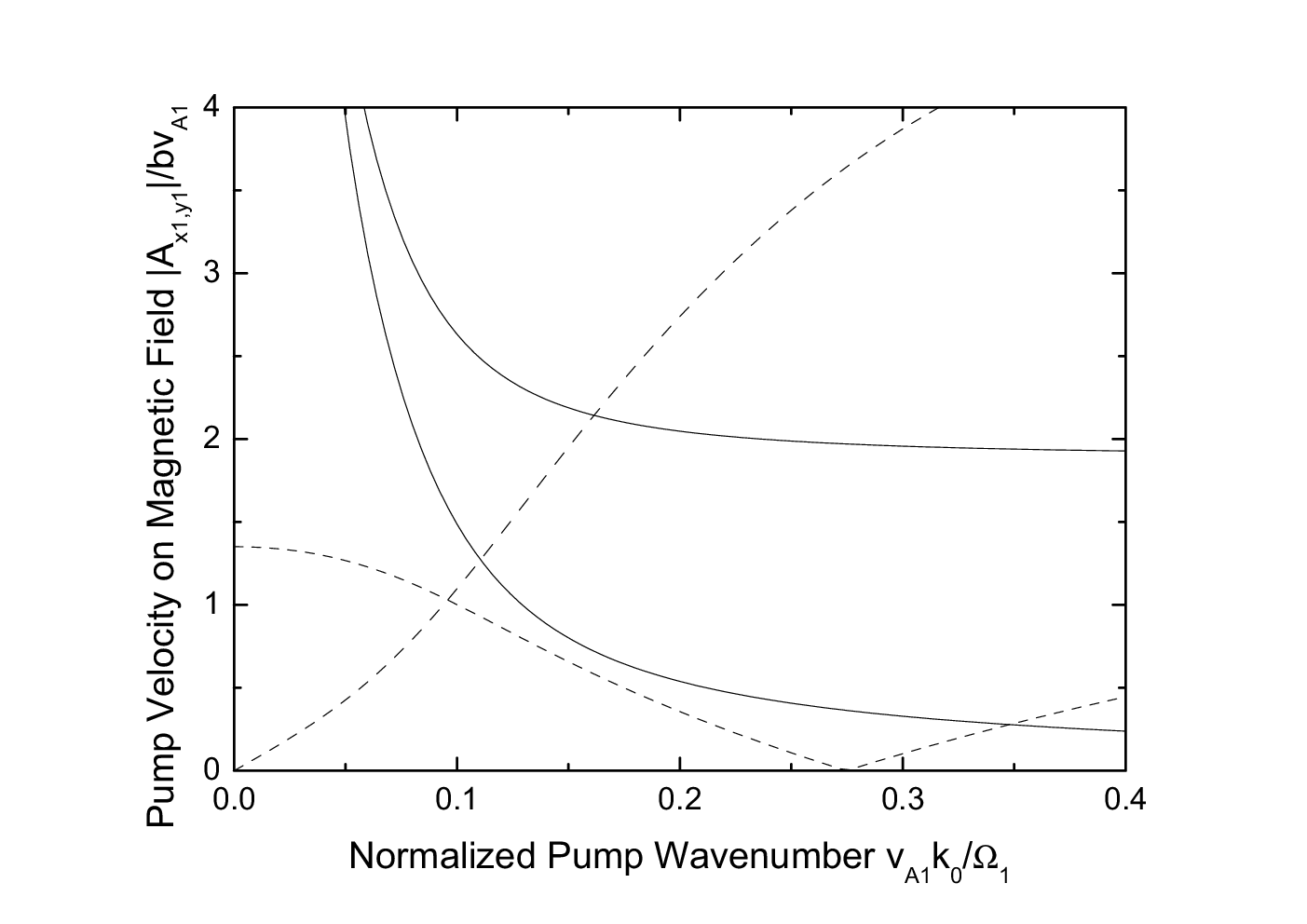
We see that as , the -component approaches a finite positive value while the -component approaches zero for the upper branch of the dispersion relation. On the other hand the -component approaches large values and the -component passes through zero for the lower branch of the dispersion relation.
Note that the two branches stemming from the upper branch of the dispersion relation become singular as . This motivates the need for a normalization condition relating the pump field amplitudes of the velocities , magnetic field , and density . A reasonable way to proceed is to assume that as we vary the energy density in the pump system is fixed. The appropriate relation in a fluid description for general magnetoacoustic waves is (e.g. Movmelrose),
| (39) | |||||
where , and the summation in the final term is over each plasma species. In our approximations the electric energy term may be neglected compared to the magnetic energy. By switching to dimensionless units and setting , then all our variables are given uniquely in terms of the basic plasma parameters. By using the expressions for and we may solve for . The result is
| (40) |
[using from Eq. (38)]. A plot of versus wavenumber is given in Fig. 3 for each branch .

It is important to note that as for the upper branch. It follows that all the velocity amplitudes are well behaved near .
The remaining pump quantities to solve for are the charge ratios . These may be obtained by imposing the charge neutrality condition on both the background plasma and on the perturbations to the equilibrium. This is justified since we are interested only with frequencies that are much less than that of the electron plasma frequency. This means the electrons have sufficient time to respond to the perturbations from the equilibrium and neutralize the plasma at each point in space. Thus, on the perturbed plasma we impose the condition,
| (41) |
where we have ignored the effects of dust (or ion) charging, that is, is constant. It is then straightforward to obtain the charge ratios in terms of the densities, and subsequently in terms of the velocity amplitudes and , as follows:
| (42) |
This implies that the amount of charge that resides on each species is temporally coupled to the other.
Using the derived set of quantities characterizing the pump wave we may, in principle, investigate the possibility of excited modes propagating at arbitrary angles with respect to the -axis, as in Ref. MovCramer76. However, by removing the -dependence in the pump waves our calculations become much more tractable, with the requirement that our excited waves are restricted to parallel propagation along the -axis, see Ref. MovCramer.
For an infinitely extended medium, the perpendicular wavenumber of the excited waves is then zero. However, this would clearly be inconsistent with wavenumber matching of a propagating pump with finite perpendicular wavenumber. We therefore envisage this analysis to apply to a standing wave (in the transverse direction) pump in a finite geometry system, such as a cylindrical or toroidal laboratory plasma, or an astrophysical magnetic flux tube; by seeking localized solutions for distances transverse to the magnetic field such that in a planar plasma, or in a cylindrical plasma, we can recover the initially proposed form for the magnetic field Eq. (18). In other words, we are taking small rather than small, to ensure that the fields will look approximately uniform in the perpendicular direction, i.e. that the wavelength is effectively very long on the length scale of interest. In the parallel direction, however, the pump fields are uniform, we place no such restriction on distances and excited wavelengths, and we can apply wavenumber matching of the excited wave fields in that direction, as discussed in Section VI.
Then in the region near the -axis we have
| (43) | |||||
| (44) | |||||
| (45) | |||||
| (46) |
correct to . Since the magnetic field has now simply a periodic variation in time it resembles a canonical parametric pump. The problem then resembles a parametric amplifier, such as a harmonic oscillator with a time-varying spring constant. For use in the excited wave equations we must also compute the derivatives near the -axis, given here:
| (47) | |||||
| (48) | |||||
| (49) | |||||
| (50) |
Note that the velocity has a finite derivative, even though the velocity itself is zero in this regime.
IV Perturbation Method
Next we wish to test the stability of the self consistent linear solution given in Eqs. (43)–(50), now regarded as a finite-amplitude pump wave, to the excitation of waves propagating along the magnetic field direction. We must however be careful since this is only a linearized pump solution. To proceed we will adopt the basic methodology of Refs. MovVahal; MovCramer, but shall attempt to refine the argument.
The basic technique is to perturb each quantity, i.e., , , , , by an arbitrarily small amount as measured by an expansion parameter . For example, take an arbitrary field, say , with a known linear representation of the pump field: . Then Refs. MovVahal; MovCramer proceed by perturbing this quantity in the following way:
| (51) |
However, since has neglected terms of , the term of is even more so negligible in this expansion (recall that is arbitrarily small). The problem lies in the fact that we are ultimately interested in the stability of the exact pump solution, say , with
| (52) |
Thus, we shall perform the following expansion instead:
| (53) |
Upon substitution into our set of nonlinear differential equations (11)–(15), we obtain a set of equations of the following structure (no approximations):
| (54) | |||||
where are differential operators acting on their respective arguments which we may treat as functions (for brevity we have suppressed their dependence on fields other than ). Now by definition of an exact pump solution. Also, the term of can certainly be neglected. Next, we Taylor expand and write
| (55) |
We are then permitted to neglect this term of when inserted back into Eq. (54). This gives us a set of equations for the perturbation , in terms of the , to sufficient accuracy, i.e.,
| (56) |
Note that has served two purposes. First, it gives us an approximate description of the corresponding exact solution , and second, it allows us to investigate its stability without ever having to find .
V Equations of Motion and Natural Modes
Our task then is to ascertain the primed variables which are the excited fields. As stated previously, we are interested only in plane waves that travel parallel to the -axis. In this case, any longitudinal components will decouple completely and merely describe a linear acoustic wave, so we may set the -component of the primed velocity to zero. Hence, both primed velocities have the following form:
| (57) |
Thus, , and from each of the two continuity equations we have
| (58) |
where we have imposed the [or ] condition. Hence we have , i.e., there are no perturbations in the densities of the excited fields. From this it also follows that .
By taking the derived expressions for , , and and substituting into Eqs. (13) & (14), and using the stability analysis procedure conveyed in Eq. (56), we obtain
| (59) | |||||
| (60) |
Here the terms of , which occur on the right hand side, should be thought of as driving terms from the pump wave. Note that there exist two further equations of motion under the index interchange . Note also that there are no acoustic terms on the left hand sides of these equations because of the decoupling of the longitudinal motions: however there are still acoustic influences in the pump fields on the right hand sides of the equations.
Now in order to treat the and components of the and vectors on an equal footing we form a complex vector out of each component of these partial differential equations, utilizing the variables . The spatial variation is assumed to be periodic in the -direction with wavenumber , as follows: . Given this, the following pair of linear ordinary differential equations are obtained:
| (61) | |||||
| (62) |
Let us define the sense of polarization in reference to the screw sense of the fields in the direction of propagation in the -direction. Then corresponds to a left hand circularly polarized wave for positive frequencies and a right hand circularly polarized wave for negative frequencies, while corresponds to a right hand circularly polarized wave for positive frequencies and a left hand circularly polarized wave for negative frequencies. Also, is defined similarly. With these definitions may be eliminated entirely from these expressions. Note that the presence of a second moving ion species introduces coupling through terms of the form: , and an additional term on the right hand side in Eq. (62) due to density variations.
In an analogous way to the classic driven pendulum problem MovPippard, we have found that the velocities of the two species satisfy a pair of generalized Mathieu equations. Furthermore, the two species and magnetic field are strongly coupled. To proceed, we move from the time domain to the frequency domain, under the Fourier transform:
| (63) |
where is the frequency of the excited waves. Using the linearity of our pair of differential equations, we compute the Fourier transform of both. Upon eliminating and in favor of , we obtain:
| (64) | |||||
where,
| (65) | |||||
| (66) | |||||
| (67) | |||||
| (68) |
and . Eq. (64) is obviously not an algebraic expression from which we can uniquely obtain the dispersion equation between and . Instead it provides us with a functional relationship between the Fourier transforms with arguments , and .
Nevertheless, we may proceed by noting that the right hand is , which is small. For the left hand side to be small we must ensure that the frequency is near a root of the polynomial on this side with a correction of , i.e.,
| (69) |
where is defined to satisfy,
| (70) |
These define the naturally occurring modes in the absence of pumping, (i.e., if then ). The solutions of these algebraic expressions give the dispersion relations characterizing plane transverse waves propagating parallel to the background magnetic field in a two species plasma. The last term of is only present when a secondary moving ion-like species resides in the plasma. It is an additional Hall-type term, associated with the relative motion of the two charged species. In the one species limit this relation simplifies to
| (71) |
and we are left with the familiar fast and slow (ion-cyclotron) transverse waves MovCramer.
The important feature of the two-species result in Eq. (70) is that it is a cubic in and hence another mode of excitation has been added. Moreover, since we may choose or it follows that there are a total of six solutions; three are left hand circularly polarized and three are right hand circularly polarized. However, only three of these are physically different. This is because if satisfies , then satisfies , and vice versa. We may then concentrate on the positive frequency solutions.
If the secondary species is positively charged then there are two left hand modes of excitation MovCrambk. These we denote by and , where the “s” denotes slow, and the “f” denotes fast. There is also a single right hand mode, denoted by . The corresponding dispersion relations are plotted in Fig. 4(a).


Note that the right hand mode intersects with the fast left hand mode. Also, the two left hand modes both experience a resonance as . For it is given by , and for it is given by (where we have assumed ).
For a negatively charged secondary species there are also three modes of excitation, however the combination of polarizations has changed. In this case there are two right hand modes and , and a single left hand mode ; see Fig. 4(b). Here has a resonance at , and has a resonance at . In the dusty plasma case, further properties of these modes were investigated in Refs. MovVlad; MovMendis; MovMeuris.
Note that the upper curves (fast modes), regardless of the sign of the species, experience a nonzero cutoff frequency which coincides with that of the pump frequency, see Eq. (30).
VI Growth Rates of Parametric Interaction
From the above analysis we see that may be any one of , , for a positively charged secondary species, or , , for a negatively charged secondary species. Since the frequency describing the excited wave is a perturbation of a natural mode frequency, we denote the change by which is allowed to be complex, where
| (72) |
Now by returning to the Fourier transform relationship in Eq. (64) we can see what effect (i.e., pumping) will have on . Without any pumping (i.e., ) the spatial solutions would be a linear superposition of three pure monochromatic exponentials. Hence the Fourier transform would be a sum of three Dirac- functions; see Fig. 5(a) for a representation.


The effect of pumping is to modify this and provide frequency shifts. The modified solution will have some broadened frequency spectrum, since it is the case that Dirac- functions do not solve the Fourier transformed equations in the presence of a pump. These types of modifications will occur near each natural frequency; see Fig. 5(b) for a simplified representation of this effect. In fact an exact solution would be more complicated with the identification of harmonics etc, but this figure should illuminate the key feature of the interaction.
This is described as a parametric interaction between the excited fields due to the pump fields. In order to proceed we consider the case in which the interaction is greatest, as in Refs. MovVahal; MovCramer. It is clear that this effect will be greatest when the right hand side of Eq. (64) is large, which is the resonance condition. This occurs when one of the Fourier transforms on the right hand side is resonant, in other words when their arguments are near one of the ’s, as conveyed in Fig. 5. Since the right hand side of Eq. (64) involves terms of the form: and , it follows that there will be a large parametric interaction when or satisfies this. Now, as mentioned earlier we are restricting our attention to positive (without loss of generality). Under this condition, it is found that only can satisfy this. Moreover, there are three choices for this interaction: a left hand mode interacting with a right hand mode, a left hand mode interacting with a left hand mode, or a right hand mode interacting with a right hand mode.
To illustrate, suppose the secondary species is negatively charged and (i.e., ). Then we can have or (left hand mode interacting with right hand mode) or (left hand mode interacting with left hand mode). In other words, the resonance condition is that the pump frequency satisfies
| (73) |
respectively, which is a statement of conservation of energy. That is, the resonance condition describes the coupling of a pump wave with two daughter waves.
Moreover, if then we can have , or and the same conditions for resonance apply. Similar rules apply for and for a plasma where the secondary species is positive.
Let us now address the issue of the treatment of the wavenumber in our pair of interacting waves. First, note that in the -direction the pump wavenumber is zero. For the natural modes we have that a wave given by is physically equivalent to a wave given by . Thus our two interacting waves will be given by and , where are any combination of . Hence the wavenumbers associated with each interacting wave are equal and opposite, i.e.,
| (74) |
which is a statement of conservation of momentum in the -direction. The fact that the right hand side is zero reflects the spatial uniformity of the pump wave. This tells us that if the approximately spatially uniform standing pump wave decays, then it does so into two daughter waves of equal wavelength travelling in opposite directions. Since the wavenumber magnitudes are equal we may just consider the wavenumber without referring to the sense of polarization. This is a direct generalization of the previous investigations in MovVahal; MovCramer; MovCrambk.
With the above framework we now proceed to solve for from the Fourier transform relationship. We discuss the method involved in obtaining in the case where a left handed wave interacts with a right handed wave, denoted . Here we may assume, without loss of generality, that in Eq. (72), where is any one of . This will interact with (i.e., may be any one of ).
Following the methodology of Ref. MovNishikawa we form another equation corresponding to (64) under the transformation . In the resulting two equations, we neglect the obviously nonresonant terms and . Additionally, due to our particular choice of interaction, i.e., left-right, we neglect and , and retain only and . We find the following:
| (75) | |||||
where
| (76) | |||
| (77) |
In these expressions we implicitly have that and , are related by: and .
In the one ion species analysis, it is at this point that the conservation of energy and momentum rules are used to explicitly obtain . The procedure is to use to solve for in terms of . These solutions are then added together and equated to . The resultant expression is then solved for and subsequently substituted into the expressions for . This process explicitly shows that the resonance condition, for a given value of pump frequency , uniquely determines the frequencies and wavenumbers of the excited waves. Now, this is all possible since the solution of in the one species limit is merely a quadratic, see Eq. (71). However, in our case we must solve a cubic. As such, the resulting expressions for are too complicated to be reproduced here. Let us just note that it is still true that determines them uniquely.
In order to solve for in Eq. (75) we Taylor expand around to order , then use the fact that , to obtain
| (78) |
where
| (79) |
while can be treated similarly. Hence is obtained from:
| (80) | |||||
Although this was derived assuming we were near a natural frequency of a left hand mode, we obtain the same expression for for the right hand case (viz. ) with the modification that is of the opposite sign.
This technique may also be applied to both the left-left interactions and the right-right interactions. This includes the possibility of a slow wave interacting with a fast wave (e.g., and ), and waves of equal frequency interacting. These sorts of interactions occur only because of the velocity derivative terms in (48) & (49). In obtaining we must retain and neglect the appropriate selection of Fourier transforms according to the choice made. Here we introduce and as two (possible equal) left hand modes, and and as two (possible equal) right hand modes. The corresponding frequency changes are obtained from
| (81) | |||||
| (82) | |||||
for the left-left and right-right interactions, respectively.
It is worth noting that in other types of parametric problems, such as modulational and beam instabilities, a graphical approach is useful in classifying the instabilities; they occur where two normal mode lines cross and reconnect MovLongtin; MovGomberoff. In those cases the number of interacting modes is finite, and the nonlinear dispersion relation can be obtained in closed form. In our case, however, we cannot obtain the nonlinear dispersion relation in closed form, due to the infinite number of interacting modes; the decay interaction of the two excited modes with the pump is postulated in the first approximation, and the classification of the instability is relatively straightforward.
VII Numerical Analysis
From the expressions for it is easy to see that these quantities are real valued when we are in a frequency-wavenumber regime such that a pump wave can propagate. Hence is either purely real or purely imaginary. If is real then what we have found is a correction to the natural mode frequency which adds an extra Fourier component to the field expansions. If is imaginary then the daughter waves will either undergo exponential growth or decay. Moreover, since there will exist both a positive and a negative imaginary frequency solution and since the frequency is conserved, this implies that one of the daughter waves will grow and the other will decay. In such cases the presence of one exponentially growing daughter wave implies that anywhere in which is a region of instability. In this case is the growth rate.
In Fig. 6 we plot the full complement of (normalized) squared frequency changes.


That is, we plot versus pump frequency for the upper “” and lower “” branches of the pump dispersion relation for each mode of interaction. This figure is for a warm plasma in which the second heavy species is positively charged. The same basic features are present in the negatively charged case. All curves labelled “”, i.e., “” and “”, correspond to the combination between and , that is the slow interaction. The curves labelled “”, i.e., “” and “”, are for the fast interaction between and .
In Fig. 6(a), where , the full spectrum of perturbations to the natural modes is seen. The interaction is unstable and monotonically decreases, approaching the single species result for large . Hence this is indeed consistent with the single ion analysis, given by
| (83) |
The interaction is also unstable, however it experiences a minimum (corresponding to a maximum growth rate), about which it turns over and approaches zero. For our choice of parameters, in this figure, this occurs near . Moreover the intersection with occurs at . Next, we see that the interaction, is small and positive, and hence it is weakly stable. Note, however, that if higher order terms are included in the field expansions then this may in fact prove to be weakly unstable. Finally, we see that the interaction, which is only present in a warm plasma, is strongly unstable, with a growth rate that approaches infinity at a rate considerably faster than or .
As we decrease the number density of the second species in Fig. 6(b) to some interesting features appear. The curve shows a sharply varying growth rate at just above the cutoff frequency. The minimum shifts to a lower value (lying beyond the range of the plot). The interaction has actually become unstable in the frequency region just above the cutoff frequency. Also, the manner in which our bi-ion result approaches the single species result as is interesting: the envelope of the three modes , , and form in the domains , and , respectively.
In Fig. 7 we plot the range of left-left interactions for the positively charged secondary species case.

As can be seen in Fig. 4(a) this case has two left handed branches (slow and fast). Hence we may form the slow-slow, fast-fast and slow-fast combinations. This combined with the lower and upper branches of the pump dispersion relation gives a total of six interactions. Of these six we find that all are unstable, except the “” combination which experiences a point of maximum stability at just below . Note that the “” interaction decreases without bound as This is acceptable given that for the slow-slow case the excited wavenumber experiences a resonance as (with pump wavenumber small). Although it lies below the range of the plot the “” interaction starts at a finite value, when . Also note the curious feature wherein the “” interaction has a corresponding growth rate which is large in the range only.
Finally, in Fig. 8 we plot the range of right-right interactions for the negatively charged secondary species case.

Again by inspection of Fig. 4(b) it makes sense that there are six values of . This plot shares many features in common with the previous plot. However, an important change is that the interactions has a minimum and approaches zero as . Also, the maximal growth rate has shifted to much higher values of pump frequency. The interaction has stability as increases.
Hence, we have seen that the introduction of a second species adds a range of extra behaviors, even with a small number density. Note that in the special case where the frequencies of different modes coincide, the selection of resonant Fourier transforms to generate these plots is actually invalid. In particular, this occurs at the point seen in Fig. 4(b) where . At that point there are actually more terms resonant than have been accounted for. However, since this occurs on a set of measure zero, it has been ignored.
VIII Conclusions
This paper has outlined an investigation into a certain class of instabilities in a bi-ion or dusty plasma, allowing full mobility of all species and the inclusion of pressure. The results should be applicable to a wide range of laboratory and space plasmas where secondary ion species or charged dust grains occur. The immediate consequence of the presence of an extra heavy species is its increase or reduction of the number of free electrons in the plasma through the charge neutrality condition. We obtained a pump wave with spatial variation transverse to the background magnetic field, which contained an upper and lower branch, and made the approximation of spatial uniformity of this pump. The stability of this structure was investigated by perturbing the pump wave, as we looked for parametric instabilities wherein the pump wave generates excited waves. Three natural transverse modes were found to be excited propagating parallel to the background magnetic field; two left handed when the second species is positive and two right handed when the second species is negative. Two out of each of these three are the modified fast and slow (ion-cyclotron) modes. There were three basic types of interactions allowed; left-right, left-left and right-right, each of which has several combinations dependent on both the choice of branch from the pump wave (upper and lower) and the choice of natural mode (slow and fast), giving rise to twelve interactions in total for any particular plasma.
We derived the frequency changes to the natural modes, corresponding to growth rates when the perturbation to the frequency was imaginary. We can summarize the main features of the instabilities for the left–right interactions (opposite sense circular polarization) as follows:
(i) Of the four combinations allowed, three are unstable when the number density of the second massive species is substantial, and all four are unstable when the number density of the second massive species is low.
(ii) As the single species case is approached (), the envelope of three different growth rates approaches it in the domains and .
(iii) The two interactions corresponding to the lower branch of the pump dispersion relation are strongly unstable, with the experiencing a local maximum and unbounded.
Next we investigated the left-left and right-right interactions (same sense circular polarization):
(i) These interactions involve six and two combinations respectively when the second species is positive, and the reverse when the second species is negative. This follows simply from the assortment of handedness of natural modes.
(ii) Of these only the interaction is stable, while the others display interesting behaviors. In particular, in the positive case, the curve approaches as where the excited wavenumber experiences a resonance, while its growth rate is maximal at just below in the negative case.
(iii) In contrast to the left–right interactions, the upper pump mode can give the strongest instabilities. The interaction has a large growth rate between and in the positive second species case, and at higher values of pump frequency in the negative second species case.
In several of the above interactions the growth rate starts at a nonzero value. This occurs in the cases where the starting value of have a corresponding nonzero value for , so the velocity derivative terms are nonzero.
A possibility for further work would be to allow the excited waves to be fully oblique, rather than simply parallel to the background magnetic field. In doing so we would be able to remove the long pump wavelength assumption, which may lead to interesting features. In the single ion case this was treated in Ref. MovCramer76, albeit without pressure. It is anticipated that implementation of the accompanying additional wavenumber matching rules, in both the and directions, would be algebraically complicated.
References
- (1) L. Spitzer, Jr., Physical Processes in the Interstellar Medium, (Wiley, New York, 1978).
- (2) W. Pilipp, T.W. Hartquist, O. Havnes, and G.E. Morfill, Astrophys. J. 314, 341 (1987).
- (3) J.I. Sakai, T.Kawata, K. Yoshida, K. Furusawa and N.F. Cramer, Astrophys. J. 537, 1063 (2000).
- (4) J.I. Sakai, R. Minamizuka, T.Kawata, and N.F. Cramer, Astrophys. J. 550, 1075 (2001).
- (5) R.J. Bray, L.E. Cram, C.J. Durrant and R.E. Loughhead, Plasma loops in the solar corona, (Cambridge University Press, Cambridge, 1991).
- (6) D. Montgomery and R. Harding, Phys. Lett. 23, 670 (1966).
- (7) G. Vahala and D. Montgomery, Phys. Fluids 14, 1137 (1971).
- (8) N.F. Cramer, Plasma Phys. 17, 967 (1975)
- (9) E. Mjølhus, J. Plasma Phys. 19, 437 (1978).
- (10) G. Morales, Phys. of Fluids 19, 849 (1976).
- (11) N.F. Cramer, Plasma Phys. 18, 749-760 (1976).
- (12) M. P. Hertzberg, N. F. Cramer and S. V. Vladimirov, Phys. Plasmas 10, 3160 (2003).
- (13) S.V. Vladimirov and N.F. Cramer, Phys. Rev. E 54, 6762 (1996).
- (14) N.F. Cramer, The Physics of Alfvén Waves, (Wiley-VCH, Berlin, 2001).
- (15) S.V. Vladimirov, Phys. Plasmas 1, 2762 (1994).
- (16) N.F. Cramer, F. Verheest, S.V. Vladimirov, Phys. Plasmas 9, 4845 (2002).
- (17) S.V. Vladimirov, Phys. Rev. E 50, 1422 (1994).
- (18) N.F. Cramer and S.V. Vladimirov, Phys. Scr. 53, 586 (1996).
- (19) K. Mio, T. Ogino, K. Minami, and S. Takeda, J. Phys. Soc. Jpn. 41, 265 (1976).
- (20) E. Mjølhus, J. Plasma Phys. 16, 321 (1976).
- (21) S.R. Spangler and J.P. Sheerin, J. Plasma Phys. 27, 193 (1982).
- (22) E. Mjølhus and J. Wyller, Phys. Scr. 33, 442 (1986).
- (23) C.R. Ovenden, H.A. Shah, and S.J. Schwartz, J. Geophys. Res. 88, 6095 (1983).
- (24) D.B. Melrose, Plasma Astrophysics, Vol. 1, (Gordon and Breach, New York, 1980).
- (25) A.B. Pippard, The Physics of Vibration, Vol. 1, (Cambridge University Press, Cambridge, 1978).
- (26) D.A. Mendis and M. Rosenberg, Ann. Rev. Astron. Astrophys. 32, 419-463 (1994).
- (27) F. Verheest and P. Meuris, Phys. Lett. A 198, 228-232 (1995).
- (28) K. Nishikawa, J. Phys. Soc. Japan 24, 916-922 (1968).
- (29) M. Longtin and B.U.O. Sonnerup, J. Geophys. Res. 91, 6816-6824 (1986).
- (30) L. Gomberoff, K. Gomberoff and A.L. Brinca, J. Geophys. Res. 107, A7, SSH 5-1-7 (2002).