Magnetic Susceptibility: Further Insights into Macroscopic and Microscopic Fields and the Sphere of Lorentz
Abstract
To make certain quantitative interpretations of spectra from NMR experiments carried out on heterogeneous samples, such as cells and tissues, we must be able to estimate the magnetic and electric fields experienced by the resonant nuclei of atoms in the sample. Here, we analyze the relationships between these fields and the fields obtained by solving the Maxwell equations that describe the bulk properties of the materials present. This analysis separates the contribution to these fields of the molecule in which the atom in question is bonded, the “host” fields, from the contribution of all the other molecules in the system, the “external” fields. We discuss the circumstances under which the latter can be found by determining the macroscopic fields in the sample and then removing the averaged contribution of the host molecule. We demonstrate that the results produced by the, so-called, “sphere of Lorentz” construction are of general validity in both static and time-varying cases. This analytic construct, however, is not “mystical” and its justification rests not on any sphericity in the system but on the local uniformity and isotropy, i.e., spherical symmetry, of the medium when averaged over random microscopic configurations. This local averaging is precisely that which defines the equations that describe the macroscopic fields. Hence, the external microscopic fields, in a suitably averaged sense, can be estimated from the macroscopic fields. We then discuss the calculation of the external fields and that of the resonant nucleus in NMR experiments.
INTRODUCTION
Overview
NMR spectroscopy is notable for its contributions to the study of the chemical and physical properties of heterogeneous samples including living cells and tissues. Variations in the magnetic characteristics of a sample often bring about readily observable changes in resonance frequency and spectral line shapes, thus providing unique probes of cellular function (e.g., 1–4). A knowledge of the physics of systems with multiple compartments of differing magnetic susceptibility has already laid the foundation for new sorts of NMR experiments. The insightful article by Chu et al. (5) explains some fundamental aspects of contrast enhancement in magnetic resonance imaging (MRI) that are brought about by paramagnetic metal–ligand complexes; and, the comprehensive review in this journal by Levitt (6) gives an independent explanation of some key phenomena. Both articles emphasize the nature and value of the magnetic field “experienced” by a nucleus in a magnetically polarizable medium. They use the theoretical construct of the, so-called, “sphere of Lorentz” in their analysis. However, this theory provoked us into some deeper questions that seemed to warrant exploration; and, with this insight came the expectation of a better understanding of experimental data and new experimental methods.
The accompanying (preceding) article illustrates the results from some simple practical NMR experiments in which samples were chosen in which there were differences in magnetic susceptibility across the (micro) boundaries of the heterogeneous samples. The experiments were conducted on solutions, an emulsion in the presence of a solution of the same substance, and a suspensions of red blood cells (RBCs) made relatively paramagnetic.
Fields in NMR
NMR spectroscopy is based on the interaction of the spin and magnetic moment(s) of a nucleus with the magnetic field in its neighborhood. To simulate NMR experiments, the magnetic field in the immediate vicinity of the nucleus in the “host” atom must be calculated. The atom itself may be free or bonded as part of a molecule or in rapid exchange between these states. In what follows, we refer to the nucleus as residing in a host molecule with the understanding that “molecule” should be interpreted as simply the host atom when it is not chemically bonded. An NMR spectrometer has a magnet that is designed to produce a strong uniform field, which we shall refer to as the applied field, into which the sample is placed. As a result of its introduction, the field in and around the sample is perturbed by the interaction of the field with the magnetic moments of the molecules in the sample. Most molecules possess no intrinsic magnetic moment because the electrostatic binding forces lead to a net cancellation of the orbital and spin angular momenta of the electrons. In the presence of an applied field, the orbital moments precess and generate an extra component that is aligned opposite to the field; this is the diamagnetic effect. On the other hand, a few atoms, ions, and molecules, in which the angular momenta of the electrons do not cancel, possess an intrinsic dipole that is much larger than the induced moment at room temperature. These molecules tend to adopt the least-energy state in which the intrinsic dipole moment is parallel to the applied field; this is the paramagnetic effect. The intrinsic paramagnetic dipole is much larger than the induced diamagnetic dipole at room temperatures, so paramagnetic molecules are often introduced as “agents” to make a deliberate modification to the applied field (e.g., 5). However, the magnetic field experienced by a nucleus in the host molecule is modified by the fields produced by all the molecules that are external to the host in which it is located and by the field produced by the host molecule itself. The former field is sometimes called the local field but because it is in the immediate external environment of the host molecule we shall refer to it as the external field. The field from the host molecule we shall refer to as the host field. The external field is dependent on the composition and geometry of the whole sample and is a macroscopic entity, whereas the host field depends solely on the structure of the particular molecule and is a microscopic entity. The change in resonance frequency due to the former is called the bulk magnetic susceptibility shift (BMS) and that due to the latter is the chemical shift. (See our preceding article for illustrations of chemical and BMS shifts that occur in samples in containers with spherical and cylindrical geometries.)
Both effects are the result of the electromagnetic properties of charges in motion and are therefore described by the Maxwell equations (e.g., 7, 8). In microscopic form, these equations describe exactly the electric field e and the magnetic induction b produced by each constituent-charged elementary particle. Hence, these equations can be used to calculate the host field and the chemical shift at a nucleus. However, it is not realistic to solve the array of Maxwell equations for all the molecules in the sample, let alone all those in the microscopic system in the vicinity of the nucleus of interest. Therefore, it is necessary to invoke a simplification that uses the Maxwell equations for the macroscopic system, and then we work down to the microscopic system. The macroscopic equations describe approximately the bulk electric field E and the bulk magnetic induction B, given the constitutive relationships between the electric field and the electric displacement D, and between the magnetic induction and the magnetic field H. These relationships incorporate the effects due to the paramagnetic and diamagnetic properties of the bulk medium, described above. But, the macroscopic field calculated using the macroscopic Maxwell equations does not provide the average field at a point where the nucleus resides within the host molecule. The macroscopic field at any point in fact contains an average contribution from the host molecule itself based on the assumption that the point is distant from the host molecule, not within it. This average host molecule field contribution must be removed from the macroscopic field to estimate the average field across the molecule due to the applied field and the contributions of all the other molecules, the external (or local) field. The actual field experienced by the nucleus is obtained by adding the external field component and the internal contribution from the host molecule, namely, the microscopic host field (see Fig. 1).
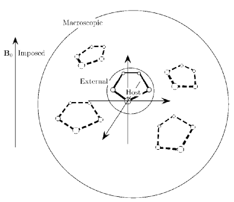
Analytic Strategy
The commonly used prescription for estimating the field at the nucleus of interest (the host field) is based on the idea of the sphere of Lorentz (e.g., 5, 6, 9). It was introduced in electrostatics by Lorentz (10) but applies equally well to magnetostatic situations (e.g., 11). It was first used in the context of NMR by Dickinson (12). The sphere of Lorentz is a notional sphere drawn around a nucleus; it is large enough for all the molecules external to it to be treated as a macroscopic continuum that is locally uniform. Within the sphere the host molecule is imagined to reside in a vacuum surrounded by individual molecules whose net electromagnetic effect is taken to be vanishingly small. The effect of introducing a spherical cavity into a uniform continuous medium is significant and yet the field arising from it can be readily calculated; hence, this provides the estimate of the external field.
The disadvantage of this approach is that it mixes the microscopic and macroscopic pictures and the justification for the field estimates at each level is not entirely clear. It has thus assumed an almost “magical” air; for example, Springer (9) writes “For an imaginary object, the sphere of Lorentz produces amazingly profound real effects.
Aims, Approaches, and Outcomes
In this article, we set out to demystify the estimation of the external fields from the macroscopic field(s). We show that the results obtained by using the sphere of Lorentz argument are in agreement with our new more rigorous approach and are of general validity. This is important because the sphere of Lorentz argument is simple to apply and can yield a semiquantitative description of BMS effects in variously shaped objects.
Our new analysis requires only that the measurement “polls” a sufficiently large number of molecules that are in random positions with respect to their neighbors for the sample average to be equivalent to the average of a single molecule surrounded by a randomized medium. Then, local isotropy, i.e., spherical symmetry, produces the same result as the sphere of Lorentz construction for a nucleus residing at its center in the otherwise empty space.
We first summarize the derivation of the expressions that describe the macroscopic fields, which are the average of the effect of all molecules present in the sample; this averaging takes place over macroscopic length and/or time scales. On the microscopic scale, all charged particles are taken to be in motion so that the electric and magnetic properties are coupled, so we must analyze the full set of Maxwell equations. It is only on the macroscopic scale that experiments can realize time scales that are sufficiently long that the macroscopic equations governing the magnetic field may be solved independently of those governing the electric field. At this stage we confine our discussion to the magnetic field in the slowly time-varying situation. Next, we examine how the average fields produced by all the other molecules at the site of a particular molecule can be estimated by using the macroscopic equations. The method of solution of the macroscopic equations is summarized in the appendix; hence, the calculation of the BMS shift in NMR experiments is completed.
The detailed treatment of the chemical shift produced by the internal field of the host molecule at any of its nuclei is beyond the intended scope of this article (e.g., 9, 12, 13) but, for completeness, we provide an estimate of the host field in the spirit of the treatment of the BMS shift so that the relative magnitudes of the combined effects can be seen.
MICROSCOPIC AND MACROSCOPIC FIELDS
Maxwell Equations
The Maxwell equations are treated in all standard texts on electromagnetism (e.g., 7, 8), so we present them with little discussion.
The microscopic electric and magnetic fields and produced by the moving charges of the submolecular particles are described by the following equations:
| (1) |
where the constants and are the electrical permittivity and magnetic permeability of free space, respectively. We must treat the microscopic electric and magnetic fields together in a coupled system because the microscopic charge density and current density vary on short time scales due to the rapid motion of the point-like charges.
The Maxwell equations are written here in their differential form using vector differential operators. The properties of these operators and their application in electrostatics are described in (14). But, their integral form is more readily visualized. Two are obtained by integrating the two equations on the left over a volume and transforming the left sides to integrals over the surface of , using Gauss’s theorem (12):
| (2) |
These are illustrated in Fig. 2.
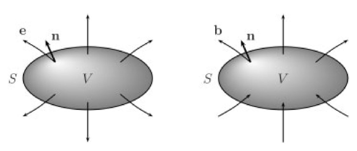
The unit vector normal to the surface at any point is denoted so that the scalar product, , is the component of in the direction normal to the surface. The first equation thus states that the normal component of integrated over the surface, the electric flux across the surface, is proportional to the total charge contained within the volume . This is Gauss’s law. The second equation states that the total magnetic flux across the surface surrounding any volume must vanish. The inward flux exactly balances the outward flux. This is due to the empirical fact that there are no sources of magnetism corresponding to point charges.
The other two forms are obtained by integrating the two equations on the right in Eq. [1] over a surface that is bounded by a closed curve , and then transforming the left side to line integrals around , using Stokes’s theorem (14):
| (3) |
Here, represents a small vectorial increment in the path around . These are illustrated in Fig. 3.
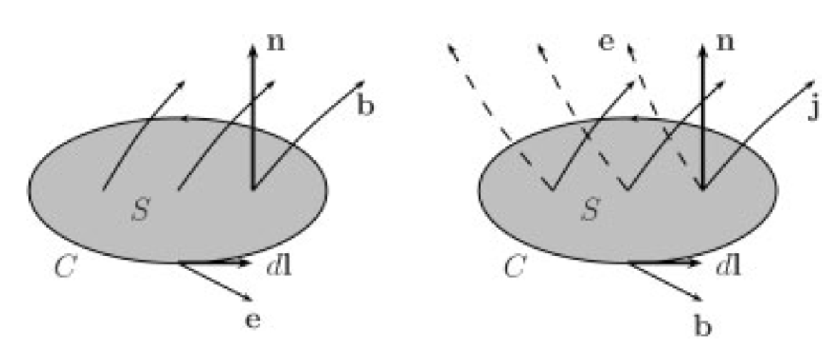
The first equation states that the line integral of the electric field around a closed path , known as the electromotive force, is equal and opposite to the rate of change of the magnetic flux across the surface . This is Faraday’s law of induction. The second equation states that the line integral of the magnetic field around a closed path is governed by two quantities. The first term on the right side is the current crossing the surface , i.e., threading . This term expresses Ampere’s law. The second term is proportional to the rate of change of the electric flux across S. This term was introduced by Maxwell, who called it the displacement current, and is essential for the existence of electromagnetic waves.
These equations can be solved by eliminating the electric field to derive the equation governing the magnetic field and vice versa. The result in each case is a wave equation with source terms provided by the electric charge and current densities:
| (4) | |||||
| (5) |
where is the speed of light. The wave equation can be solved formally in terms of an integral, over all space and all time, of the sources on the right sides of these equations. They admit both “advanced” and “retarded” solutions, i.e., one in which the effect of the source propagates backward in time with the speed of light and one in which it propagates forward in time. The advanced solution is discarded to avoid violating causality. The resulting retarded solution can then be expressed as an integral over all space of the contribution from every source at the retarded time. This time is simply the time at which the electromagnetic signal, traveling at the speed of light, must have left the source point to arrive at the selected point of space where the fields are measured at the selected time .
This formal integral solution can be written in a variety of different ways. The Jefimenko form (e.g., 7) is one of the most illuminating:
| (6) | |||||
| (7) | |||||
Without the final term, Eq. [6] is Coulomb’s law and, again without the final term, Eq. [7] is the Biot–Savart law. In these equations, is the retarded time referred to above, and the integration is taken over all of space. In the steady state, only the first terms of the right side of Eqs. [6] and [7] appear, so that the electric field is seen to depend only on the charge distribution, and the magnetic field depends only on the current distribution. The size of the second term relative to the first is 1:(), where and are the characteristic distance and time scales of the system. If the system changes only slowly (viz., over time scales long compared with , the time for light to travel a distance ), the second terms and the variation in the retarded time can be neglected; we call this situation the quasisteady case. At the microscopic level, the time scale is determined mainly by the orbital speeds of the electrons that are an order of magnitude less than c. At the macroscopic level in NMR experiments, the time scale is governed by diffusion, i.e., the thermal speeds of the molecules and these are many orders of magnitude smaller than c. The quasisteady approximation is, therefore, good in the latter case, but more care needs to be taken at the microscopic level.
We now focus on the conceptual steps involved in proceeding from the microscopic picture in which the molecular constituents of the material are described as charged particles in motion in a vacuum, for which the solutions can be written down exactly, to the macroscopic picture, which involves systematic averaging over the sample. Only by doing this is the relationship between the two pictures revealed. Because there are several steps that are mathematically independent but logically connected, we use a notation that, although somewhat cumbersome, does help keep track of the steps.
Temporal and Spatial Averages
The development presented by Jackson (7) is based on Russakoff (15) and we follow his approach here: The Maxwell equations are linear so they can be averaged over space or time to describe the average microscopic electric and magnetic fields and . These are expressed in terms of the sources of the fields, which are the charge density and current density that are averaged in the same manner, namely,
| (8) |
The form of these equations is precisely that of Eq. [1] so that the integral forms and the general solution applied to the averaged fields in the sources are replaced by the averaged sources.
Significance of Linearity
The property of linearity enables the fields to be obtained by averaging the sample point over a volume in space or interval in time; this is precisely the value of the field that would be obtained if it were measured at a fixed point but arose from sources that were averaged over an equal volume or equal time interval. As a further consequence of linearity, the average fields and sources of any system are equal to the sums of the average fields and due to the average sources and representing each of the molecules present in the system. Specifically, . Thus, each average molecular field is described by the Maxwell equations, Eq. [8], with the corresponding average molecular sources.
Suppose that the th molecule consists of charged particles, namely, electrons and protons; it also contains neutrons that generate no electromagnetic effects per se. We shall not be interested in following the submolecular motion, so we first average over a time scale that is long compared with that of the orbital motion of the electrons but short compared with that of the motion of some reference point (usually taken to be the center of mass) of the molecule. We denote any time-averaged value of a property with an overbar:
where the temporal smoothing function is normalized so that and it vanishes for time scales longer than that of the submolecular motion. By treating each submolecular particle as a discrete point charge, the charge and current density due to the th charge in the molecule can be expressed in terms of a delta function (which has, it should be noted, units of volume-1) as
| (9) |
Here, and are the position and velocity of the center of mass of the th molecule; is the charge of the th submolecular particle in this th molecule; and and are the position and velocity of the th submolecular particle with respect to its center of mass (see Fig. 4).
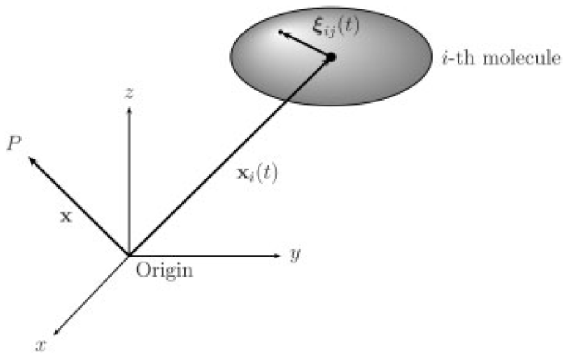
The delta function is a convenient mathematical device for representing a point particle. This function vanishes everywhere except at the point , yet its integral over any volume containing the point is unity. Hence, the quantity is a charge density such that the total charge if the point charge at is outside the volume and the total charge if the point charge at lies within . Likewise, the quantity is a current density such that the current if the moving charge at lies outside and the current if the moving charge at lies within . Here, is just the rate at which the point charge is moving; because its position vector is a function of time, , its velocity is .
Multipole Expansion
At a point external to the molecule the inequality holds, so we can expand the expressions in Eq. [9] as series in terms of increasing powers of the small quantity . This procedure leads to a multipole expansion. Normally, higher-order terms are small enough to be negligible compared with the first one or two terms. Truncation of the series after the second term is referred to as the dipole approximation and it yields the following expressions for the total charge and current densities for the th molecule:
| (10) | |||||
| (11) | |||||
where the total molecular charge (independent of time), electric dipole moment , and magnetic dipole moment are defined by
| (12) |
The significance of each of the remaining terms will be explained below but, in the meantime, these expressions suffice to convey the idea that when averaged over time the whole molecule appears at distant points as if it were a point object. However, it is conceptually convenient in what follows (although not mathematically imperative) to restore the finite extent of the molecule when we deal with its immediate neighborhood. Thus, we smooth the ith molecule over a volume that is comparable to the volume that it occupies. The spatially smoothed quantities are denoted by a double overbar:
where describes the form of the smoothing function around . It vanishes outside and is normalized so that its integral over is unity.
The Maxwell equations written with these averaged sources describe fields that vary smoothly over length and time scales greater than those of the submolecular structure. However, the sources and fields still have features on the scale of intermolecular distances. The macroscopic equations are based on eliminating this fine structure by being smoothed over a volume V of space that is sufficiently large to contain a large number of molecules. These newly smoothed quantities are denoted by angular brackets:
where is another normalized function, like a Heaviside step function, that vanishes outside .
The macroscopic averaging process warrants some discussion. It is implicit in this concept that the result will describe a physical system that can be measured with macroscopic equipment and produce repeatable results, at least within an acceptable error range. As a result, the macroscopic average must be made over a volume large enough to ensure that the movement of the molecular constituents both within this volume as well as in and out of this volume results in little change to the average properties. Further, the average should reflect the results of measurement by different instruments that may sample the volume in a similar, but not identical, manner. So, the macroscopic aver- age should not weight heavily any localized region within itself. It is therefore logical, as well as expedient because it simplifies the mathematical treatment, to take the smoothing function to be uniform over V so that . Thus, we restrict the integration to the volume around , writing
| (13) |
Combining all smoothings, the average charge and current densities become
| (14) | |||||
| (15) | |||||
where
Thus, the charge sources are contributed by the molecular charge density and spatial variations of the electric dipole density; the current sources are contributed by the molecular charge flux, temporal variations of the electric dipole density, and spatial variations of the magnetic dipole density and the electric dipole flux density.
Finally, the macroscopic charge and current sources are obtained from Eqs. [14] and [15] by summing over all molecules. Hence,
| (16) | |||||
| (17) | |||||
where the macroscopic polarization and magnetization are defined to be
| (18) |
At this stage of the analysis, we made the usual assumptions that the molecular charges and charge fluxes sum to zero over a macroscopic volume, so the expressions for both the average charge density and average current density depend solely on the dipole terms. The second term in the expression for the average current density is the spatial average of the (vector) product of the dipole moment and the center-of-mass velocity of the molecules. If there is no correlation between the dipole moment and the velocity (one is microscopic, the other is macroscopic) then the average of the product is equal to the product of the averages. In this case, if there is no bulk motion in the system the average velocity of the center of mass vanishes and the macroscopic current density reduces to
| (19) |
This yields the Maxwell equations that describe, within the approximations detailed above, the macroscopic fields and in their standard form in the absence of free charges:
| (20) |
These equations should be contrasted with the original microscopic form in Eq. [1]. They have exactly the same structure but the source terms are no longer discontinuous functions of the microscopic charges and of the currents produced as they move. Instead, the sources are continuous functions of the electric and magnetic dipole densities, which are the highest-order terms to survive the averaging processes. However, the general solution of these equations is the same as for the microscopic equations given by Eqs. [6] and [7] with the appropriate change in the expressions for the source terms. In the quasisteady case these are
| (21) | |||||
| (22) | |||||
In practice, these are just formal solutions because the dipole moment densities are, in general, not prescribed functions of space and time. Following Maxwell, we must therefore proceed by introducing the new fields
| (23) |
Then, the new Maxwell equations assume the standard macroscopic forms:
| (24) |
We now have four vector field quantities, i.e., 12 scalar quantities, to determine from only eight component equations. This is impossible without additional information about how the four fields are related to one another. But, before considering this question, we can use the prescription for obtaining the macroscopic equations to answer the fundamental question of how such fields can be used to estimate the fields experienced at the site of a constituent molecule, i.e., to calculate what we have defined to be the external fields.
EXTERNAL FIELDS
Key Concept
The key concept in understanding the theoretical construction derived in this article is: The external fields at the site of an individual molecule within a sample differ from the macroscopic fields as calculated above because the macroscopic field already contains an averaged contribution to the fields from the molecule itself. It is obvious that the macroscopically averaged fields experienced by the kth molecule are found simply by solving the macroscopic equations, with sources from the averaged contribution of that molecule subtracted. It is not obvious, however, that the actual external fields will always be such fields obtained by macroscopic spatial averaging. Indeed, in crystals, they may never be.
Crystals
In the case of a crystal with molecules arranged in a regular lattice, there will be no spatial smoothing and the external fields will be similar for all similar molecules and could differ greatly from the macroscopic average. The external fields can only be estimated by solving the full set of microscopic equations for the whole lattice; however, this problem is not discussed further here as it is not pertinent to molecules in solution.
Amorphous Solids
In an amorphous solid, with random structure, an individual molecule also does not experience spatially smoothed external fields. Consider a group of like molecules with random arrangements of their neighbors in a volume . If this volume is used to define the macroscopic average then the external field experienced by the group will be similar to the macroscopically averaged field. The mean field experienced by a smaller group (in a smaller volume) will, in general, differ from the macroscopically averaged field because the system will retain structure on the scale of intermolecular distances. The evaluation of the external fields in the latter case poses an intractable problem.
Averaging Process for Fields and Sources
The question of how to estimate the mean external field thus hinges on the nature of the averaging process. Recall that linearity implies that averaging fields is equivalent to averaging the sources. In a fluid, the molecular sources move around, so a temporal average is equivalent to averaging over the locations of the molecules, i.e., to spatial averaging around a fixed site. This is the ergodic hypothesis of Boltzmann and is plausible, although difficult to prove rigorously in most cases. If a finite volume containing a large number of molecules with host atoms is sampled, each such molecule will be surrounded by other molecules in a series of random realizations. The external field, averaged over such an ensemble of realizations, is again equivalent to a spatial average around a fixed site. The distribution of surrounding sources is then locally uniform and isotropic within the averaging volume V. This property characterizes the macroscopic average and defines how large the necessary macroscopic averaging volume should be. We shall consider this case exclusively.
Focus on this averaged spatial distribution of sources in the neighborhood of an individual molecule, labeled . To maintain the identity of the molecule, we assume that it occupies a volume Vk about the “center” of the molecule at ; all other molecules are excluded from this volume. We now smooth the molecules outside this volume over a spherical volume to produce a continuous distribution that maintains the volume free of sources. As before, we shall take the smoothing function to be uniform over . If does not contain , the sources will be averaged over the whole of so that at points inside and outside. Then, the spatially averaged sources contributing to Eqs. [14] and [15] will take the form
| (25) |
The prime on the sum indicates that the term must be omitted. The second expression follows from the first because vanishes throughout . It is precisely the definition of the macroscopic average in Eq. [13].
Smoothing Over Sources in the Neighborhood of a Host Molecule
If we smooth (average) over a volume that includes any part of we must confine the sources to the volume minus , which is that part of within (see Fig. 5).
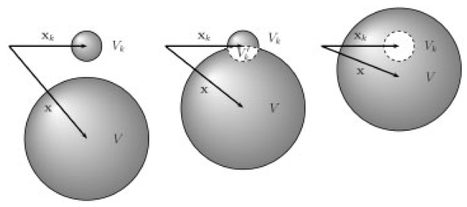
This volume depends on the position of the center, , of the smoothing sphere relative to the center of the molecule . The normalization now gives and the average sources are
because vanishes throughout . This does not match the definition of the macroscopic average but it can be further expressed as
Now, the first integral is the total source within . Because is the macroscopic volume, this source is given by Eq. [25] as . The molecules will be randomly distributed over this volume with an average number density , where is the average molecular “volume” so we can define the average source associated with each molecule to be
unless the total source vanishes, i.e., . The second integral is the source due to the th molecule within . By definition, the source within is
If is uniform within , then it follows that
If is not uniform, we can always write,
where is some smooth function of position with respect to the center of the molecule and is a function of the structure or shape of the kth molecule. When all the molecules are of the same type ; otherwise, we write , where is a proportionality constant that depends on the other molecular structure(s). Then, substitution yields
if . This case describes the contributions of the molecular dipoles and to the sources in Eqs. [14] and [15]. When ,
This case describes the contribution of the possible molecular charge to Eq. [14] because
At locations within we must, of course, set .
Alternative Representation of the Sources
The results of the previous section can be put in an alternative, perhaps more illuminating, form by noting that they differ from the sources for the macroscopic fields only within or when includes some part of . The external fields are therefore obtained from the macroscopic fields and by removing the fields due to the contribution of the th molecule to the sources within , and around . We call these the self-fields. They are produced by the sources, as follows:
or, if ,
The shape functions,
| (28) |
contain all the effects of the particular structure of the kth molecule. The other quantities are all macroscopic quantities.
The expressions for the self-fields then result from solving the Maxwell equations with charge densities:
and current densities:
Prescription for External Fields
The previous section provides a prescription for evaluating the external field experienced by an individual molecule due to a surrounding randomized configuration of other molecules. The equations may be solved if the structure and dynamics (position, orientation, and velocity) of the molecule are known. In practice, the dynamic state of individual molecules will not in general be known, so this formalism has limited utility. However, in NMR experiments the signal is generated by a large number of nuclei residing in molecules, all in different dynamic states. Therefore, we can perform another averaging: This time it is done over the velocities and orientations of the host molecule. If there is no net flux of the molecules in question, i.e., there is negligible bulk motion, the velocity-dependent terms will average to zero. If we also average over all orientations then the newly averaged sources must be distributed with spherical symmetry. The host molecule is thereby replaced by one that is spherically symmetrical, as in Fig. 6.
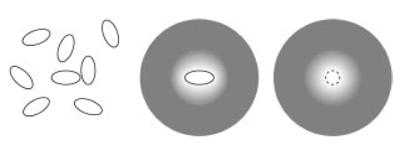
The molecular volume will then be a sphere and all spatially dependent factors in the shape functions will depend only on distance from the center at .
If we recall that the point is some reference point in the molecule, not necessarily the center of mass, it is clear that we can now choose that point to be the location of the nucleus in the host molecule. When the orientations of the molecule are averaged about this point, the averaged sources due to all the other molecules become spherically symmetrical about the nucleus. The average fields experienced by that nucleus are those due to the spherically symmetrical source distributions, evaluated at the center, i.e., at .
We can now construct the sources explicitly. Letting be the radius of , and the radius of , the charge densities are given by
and the current densities are given by
where and are the macroscopic polarization and magnetization around .
Isolated Molecules
Consider the idealized case in which there is a single molecular species (so and ) and set and so that each molecule occupies the same exclusive spherical volume that is equal to the molecular volume. Then, the shape functions vanish, leaving only the uniform sources and within . Substitution into the quasisteady expressions Eqs. [21] and [22] yields explicit estimates of the selffields at that are given by
| (32) |
The contribution from the polarization to integrates to zero at the center of the sphere. This does not occur at other points within the sphere. However, in the strictly time-independent case the fields are uniform within a sphere with uniform polarization and magnetization so Eq. [27] gives the estimate of the static self-fields at all points within the sphere. This case reproduces the result obtained from the sphere of Lorentz construction, even though the spheres are differently conceived and are of different size. The contradictions inherent in this simplistic view of the sphere of Lorentz are apparent, however, so we pursue the rigorous treatment.
Rigorous Treatment
If we wish to identify values averaged over V in the general case with the macroscopic averages, we must take . The macroscopic sources are then uniform throughout and its surroundings, within the much larger volume about the molecule. Thus, in the surrounding shell only the shape functions vary and then only with respect to the radial coordinate . The importance of this property was noted by (6); substitution of these forms in Eqs. [21] and [22] produces exactly the same estimates as those in Eq. [27] for the fields at the center of Vk. Away from the center, the time-varying polarization will again contribute to Bself. In the strictly time-independent case, the fields will again be uniform throughout , so these estimates will apply at all points within .
The external fields experienced at any position within an averaged molecule in averaged surroundings are the macroscopic fields less the self-fields. In the static case, these are
| (33) |
In the time-varying case, these expressions are exact at the center of the symmeterized molecule and approximate the fields close to the center.
The most significant conclusion, however, follows from the fact that the nucleus of the host molecule is placed, by construction, at the center of the symmeterized distributions. The expressions in Eq. [28] therefore give the average fields experienced by the nucleus as a result of the surrounding molecules exactly, even if the fields are not static.
Alternative Expression for the External Field
An alternative form for the expression for external fields can be obtained by recognizing that our assumptions allow us to rewrite Eq. [18] as
| (34) |
where is the number density of molecules and and are the mean molecular electric and magnetic dipole moments in the sample. Then,
| (35) |
In the case of diamagnetic and paramagnetic molecules, which are of considerable interest in NMR experiments, the external fields experienced by a molecule determine its microscopic (molecular) electric and magnetic dipole moments. The mean moments of all the molecules in the sample are linearly related to the external field by the expressions
| (36) |
where is the average molecular polarizability and is the average molecular magnetizability; these quantities are provided by the analysis of molecular dynamics and have the dimensions of volume. (Note that these , parameters are not the magnetogyric ratio that is usually denoted by this symbol in NMR theory.) Substituting for the external fields from Eq. [30] it is seen that the moments are aligned with the macroscopic field:
| (37) |
The polarization and magnetization are therefore
| (38) |
and
| (39) |
Susceptibilities
When calculating macroscopic fields, it is more usual to introduce the susceptibilities and , which are defined by
so that
| (40) |
where and are the permittivity and permeability of the material, respectively.
Thus, in terms of the susceptibilities, P and M are given by
| (41) |
hence,
| (42) |
The external fields can now be evaluated directly from the macroscopic fields using Eq. [37], where the macroscopic fields are found by solving the Maxwell equations, Eq. [24], together with the constitutive relations, Eq. [35].
Review
So far, we have developed the theory of external fields for both the electric and magnetic fields for several reasons. First, it is based on a model of microscopic charges for which the electric and magnetic fields are strongly coupled because of the rapid motion of the submolecular particles. Second, the macroscopic fields remain coupled, but much more weakly because the macroscopic motions are much slower than the microscopic ones and produce changes in the macroscopic properties only over much longer time scales. Third, the external fields can be analyzed systematically when both the magnetic and electric fields are varying slowly, the analysis leading to the remarkable generalization of the sphere of Lorentz construct to cases in which time variations are present. The results of the construction may therefore be used when an electric field is imposed on a sample in an NMR experiment or when the applied magnetic field fluctuates.
We can therefore safely adopt the simplification made in most NMR applications that the system is in a macroscopically stationary state because any real deviations from this state will not affect the manner in which the external fields can be estimated. The advantage of the stationary assumption is that the equations governing the electric and magnetic fields are then decoupled, allowing one to be treated independently of the other. Therefore, in the examples that follow to illustrate the theory attention is restricted to the static magnetic field. Then, the calculation of the external magnetic field from Eq. [37] requires a knowledge of the expression for the macroscopic field . This is found via the macroscopic Maxwell equations; the time-independent forms are
Their formal solution is treated in standard texts such as (7, 8) and an outline in the context of NMR is given elsewhere (e.g., 16) and in the appendix.
HOST FIELD
General
The macroscopic fields, and the fields from the charged particles, are calculated using the approximation in Eqs. [10] and [11], which is appropriate for points at a large distance from the system of charges that constitute each molecule. When calculating the fields experienced by the nucleus of a host molecule, there are contributions—the host fields—from the system of charges constituting that molecule. This situation requires us to evaluate the fields at an internal point of the host molecule. Due to the proximity of the electrical and magnetic field sources, these fields will in general be more intense than those generated by the other, distant, molecules. Their effect on the NMR resonance frequency of a nucleus, called the chemical shift, is likely to be greater than that of the external field, which produces the bulk susceptibility shift. The host fields must therefore be determined with care for each atomic nucleus in each molecular species and it requires the full panoply of quantum mechanics. This has been applied by many authors from Ramsey (17) onward and is beyond the intended scope of this article. However, the effect may usefully be illustrated by a simple model.
Simple Model
In the absence of an applied field, there will be no preferred direction for a molecule and so the averaged sources will have a distribution with spherical symmetry about any fixed reference point, the nucleus in the host molecule, for example. Suppose first that the nucleus is at the center of a host atom so we assume that the positive charge resides at the center. The negative charge due to the averaged electron cloud will appear as a spherical shell around it. In the presence of an external field, the first-order perturbation of the spherical shell will be a dipole term with its axis in the direction of the applied field. Take the preferred direction to be that of the unit vector . We can take the nucleus as the origin of the coordinate system without loss of generality. Then, the mean charge density due to the electrons about the nucleus can be written as
where is the distance of the point from the center. The charge density is here a negative quantity and the center of the distribution is shifted in the negative direction due to the Lorentz force due to the local applied field. The mean current density can likewise be written
Note that the spherically symmetrical current term vanishes and the first-order term is a circular current system about the axis . When is positive this represents a paramagnetic effect; when negative, it represents a diamagnetic effect.
The quasisteady microscopic host fields at the origin are found by substituting these forms into the appropriate terms of Eqs. [6] and [7] and performing the integrations, giving
We can also evaluate the average electric and magnetic dipole moment of these distributions from
The electric dipole is always oriented antiparallel to the applied field and the magnetic dipole is parallel to the applied field for paramagnetic molecules and antiparallel for diamagnetic molecules. Hence,
The internal electric field is always antiparallel to the electric dipole moment and the internal magnetic field is always parallel to the magnetic dipole moment. The exact relationship between the dipole moments and the internal field, of course, depends on the electronic structure of the molecule. The result can be written in terms of the effective volumes of the molecule and , defined by
| (43) | |||||
| (44) |
Similar expressions will therefore arise in the more complicated cases that occur when the host atom is chemically bound to a molecule. Averaging all possible orientations of the molecule will produce charge and current distributions with spherical symmetry about the reference point, which is the nucleus of the host atom. The external field will produce first-order perturbations of these distributions that give rise to net dipole moments and to the related host field at the nucleus (center) of the host molecule.
DISCUSSION
Sphere of Lorentz Argument
We have shown above that the sphere of Lorentz construct does indeed provide a means of estimating the fields, both electrical and magnetic, at points within a molecule embedded in a macroscopic sample composed of other molecules. Our derivation does not depend on an ad hoc “hard” spherical construction but it can be viewed as sort of “soft” spherical one. The analysis demands that we do not attempt to estimate the fields experienced by an individual molecule, but we estimate the average fields experienced by a large collection of similar molecules so that both the dynamic properties of the molecule and the locations of the neighboring molecules are randomized. Under these circumstances, the microscopic electromagnetic sources in the close vicinity of the molecule display spherical symmetry, as do the macroscopic ones. It is the assumption of spherical symmetry that produces the general results described by Eq. [28], not sphericity. This explains why the radius of the assumed sphere of Lorentz plays no role in the result; the properties within a sphere of any radius drawn around the center of a molecule will be symmetrical and lead to the same result. Our argument is, however, not independent of the distance scale so the size of the averaging sphere is not totally irrelevant. The macroscopic properties of the material are required to be locally uniform, so the size of the macroscopic smoothing volume must be chosen to ensure this apparent homogeneity. This volume must be sufficiently large to randomize the contribution of the least abundant molecular species. Therefore, the smoothing volume will be least when all the molecules in the sample are of the same species. For a macroscopic model to make sense, this volume must be less than that of any macroscopic heterogeneities. Such cases will be illustrated in the examples below.
Chemical Shift
The magnetic field experienced by a nucleus in an atom in a molecule is dependent upon the local bonded structure of the atom. This field is the basis of the experimentally important chemical shift of the intrinsic resonance frequency away from the value that pertains to the isolated atom. In what follows is an explanation of this phenomenon and a model of a molecular system that provides an estimate of the order of magnitude of the chemical shift effect relative to that of the BMS shift.
It is immaterial whether the host atom, in which the nucleus of interest is located, is chemically bonded into a larger molecule or not. In either case, the nucleus will experience, on average, fields that are the sum of the external fields, Eq. [28], and the host fields, Eq. [39]. The size of the host fields will, of course, depend on the molecular environment of the host atom. Nevertheless, the dipole moments of the atom or molecule to which it is bonded are linearly related to the external fields as in Eq. [31] but with the mean molecular polarizability and magnetizability replaced by the quantities specific to the type of molecule in question, say. Carrying out these substitutions gives the host fields at the nucleus, Eq. [39]:
Then, we find the total fields at the nucleus to be
where and are the macroscopic fields. These can be put in a more revealing form by writing in terms of the mean polarizability as
| (45) |
and similarly for the magnetizability. Then,
| (46) | |||||
| (47) | |||||
Now, is the number of molecules per unit volume so is the ratio of the average intermolecular volume to the volume of the molecule, as defined by Eq. [38]. In fluids this ratio is, say, of the order of 10, falling to unity when the molecules are densely packed. The other factor is the ratio of the specific to the mean value of or . If there is only a single species present, this ratio is unity so the chemical shift due to the host field contribution will be an order of magnitude greater than the bulk susceptibility shift due to the external contribution. If the molecules are diamagnetic then in the host field and this reduces the field experienced by the nucleus; so, the effect is referred to as diamagnetic shielding. If the molecule is paramagnetic, and the nuclear field is enhanced. When there are several species of molecules present, the host contribution depends on the properties of the molecule in question relative to the average. It will be greatest when the molecule to which the host atom is bonded is strongly paramagnetic while the mean is weakly diamagnetic. These considerations simply emphasize the need to have accurate estimates of the host field at the site of the nucleus of the host atom when the molecule is averaged over all orientations. In this situation the required analysis of chemical shifts is sophisticated and computer intensive (e.g., 9).
ILLUSTRATIVE EXAMPLE
In the following we illustrate the theory by evaluating the external field and the susceptibility shift in a suspension of RBCs following the procedure outlined by Wolber et al. (18).
Susceptibility-Induced Shifts
These authors begin their analysis with a system in which a uniform strong magnetic field B0 is created in a material of susceptibility . There is then uniform magnetization in the material given by Eq. [36]. If a sample with susceptibility is now introduced then the new field will be the sum of the original field and the field due to the change in magnetization
| (48) |
inside the sample and
| (49) |
outside the sample. But, also satisfies the following equation (see appendix, Eq. [75]) for the case of a single surface :
| (50) |
where is the surface of the sample. As noted in the appendix, these equations do not provide a full general description of the field. For a full solution, it is usual to solve the Laplace equation, Eq. [77], with appropriate boundary conditions, for the scalar potential (e.g., 16). However, Eq. [45] does provide a useful approximate form of the expression when the magnetic susceptibilities are small. In practice, is of the order of cgs-emu ( SI units) so that is also of order . Hence, to first order in small quantities we can write
| (51) |
inside the sample and outside. Again, to first order,
| (52) | |||||
The new macroscopic field inside the sample is thus, approximately,
| (53) | |||||
The integral over the surface of the sample is a function solely of the geometry of the surface. In general, it is a function of the position x of the point within the sample. For ellipsoidal surfaces (including the special case of a spherical surface), however, the result is independent of ; in other words, the field within the sample is uniform. For a sphere,
| (54) |
so the macroscopic field is
| (55) |
In general, we may write
| (56) |
where is the geometric demagnetizing factor that is described by (18) among others; and, for a sphere . For an infinite cylinder aligned at right angles to the field, . Of course, there is no surface effect for a cylinder aligned parallel to the field and . A table of such factors is provided by Chu et al. (5). The geometric factor is the same at all points within these objects and in all objects with ellipsoidal surfaces (16); the field is therefore uniform within them. For other objects, the geometric factor will be a function of position and the field will not be uniform. In either case, we can write the macroscopic field as
| (57) |
and the external field as
| (58) | |||||
to first order in the susceptibilities. This expression describes the external field in absolute terms, i.e., it is the field experienced at a point surrounded by a local vacuum in the sample. The expression agrees with (5) but it agrees with Eq. [1] in (18) only if the original material is taken to be a vacuum, i.e., .
The difference arises from the focus of the latter authors on the frequency shift observed in NMR experiments. This shift is governed by the change in the external field as a result of introducing the sample. Before the introduction the macroscopic field is so the external field at the site of a nucleus is approximately
while the external field at the site after the introduction of the sample is given by Eq. [53]. The change is therefore
which is Eq. [1] in (18).
Sample Heterogeneity
Wolber et al. (18) also consider the case in which the sample is heterogeneous, consisting of plasma and RBC. If the magnetic field in the sample is averaged over a volume large enough to contain many erythrocytes, the system can be considered to be uniform with a volume-average susceptibility given by
| (59) |
where the subscripts and denote erythrocyte and plasma, respectively, and is the average volume of an erythrocyte and the average volume of plasma surrounding each erythrocyte. The macroscopic field that determines the external field at a nucleus can then be calculated as outlined above from the averages bulk properties. If sample size is not large compared to the size of the heterogeneities in the system, account has to be taken of the detailed distribution of erythrocytes in the neighborhood of the nucleus in question. To do this, these authors conceptually surround the site by a sphere, , that is comparable in size to the averaging volume (see Fig. 7).
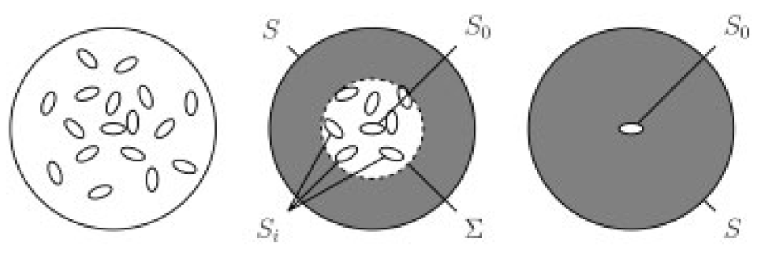
The field source outside this sphere contributes at the center an approximate field, called the “far” field, that is described by
| (60) | |||||
the normal being directed out of the sample in the first integral and into the sphere in the second. As a result, the two terms will almost cancel one another if the averaging volume is comparable to the sample volume; however, the purpose of the construction is to place as much as possible of the sample outside the surface so that it can be treated in an average manner. Using the results from above, these expressions yield
| (61) | |||||
This is the generalization of Eq. [3] of (18) for . To this must be added the “near” field contributed by sources within the sphere; this field is estimated by taking an alternative macroscopic average over a volume smaller than that of an erythrocyte but larger than that of any internal structures. This construction ensures that the susceptibilities and are uniform within the erythrocyte and the surrounding plasma, respectively. The macroscopic system is thus divided into a hierarchy of macroscopic systems, each of which contribute to the macroscopic field at the site of a nucleus. Then, the changes of magnetization within the spherical volume, which are given by
| (62) |
produce an approximate near macroscopic field at a point in the plasma of
| (63) | |||||
| (64) |
Here, the sum is taken of the integrals over the surfaces of all the erythrocytes within the sphere with the normal at the surface pointing into the erythrocyte; and, the final term is the integral over the surface of the surrounding sphere with outwardly directed normal. The susceptibility at points on this sphere will vary according to whether the point lies in plasma or erythrocyte. However, the sphere will, by construction, intersect a large number of erythrocytes and so the integral may be approximated by replacing by the average bulk susceptibility on the surface. In this approximation
| (65) |
which, of course, cancels the contribution of the surface of the sphere to the field .
The near contribution to the macroscopic field in an RBC is, in the same approximation, given by
| (66) | |||||
| (67) | |||||
| (68) |
where is the surface of the selected RBC and the sum is taken over all the others ( in total) in the sphere, the normal now pointing out of each RBC. The first integral is evaluated at an internal point and can be treated as before in Eq. [51], replacing s by , which is the geometric factor appropriate to the shape of the RBC. The integral over the sphere is treated as before but it appears to have been omitted by (18). After making this correction, the total macroscopic field at a point in an RBC is
| (69) | |||||
where
| (70) |
To first order in the susceptibilities, the external field experienced by a nucleus in an RBC will be
| (71) | |||||
This expression corrects and generalizes Eq. [5] in (18). These authors introduced a further term to describe the contribution of the particles within a sphere of Lorentz drawn about a nucleus within the RBC; then, they argued that it vanished “because of symmetry.” We have shown above that the contribution is in fact included in the estimate of the external field if the particles are randomized within the “local” macroscopic volume that surrounds the nucleus, so the final result is the same.
Wolber et al. (18) then claim that vanishes due to symmetry. However, in general, there will be no symmetry in the distribution of the other RBCs about the selected cell. An exact evaluation is then impossible. We argue that this contribution can be estimated only if the experiment samples enough RBCs (either in volume or time) that the configuration external to any individual RBC is randomized. Then, the structured medium can be replaced by a homogeneous medium with a mean susceptibility given by Eq. [54]. In this case
and the external field becomes
| (72) | |||||
Of course, this is exactly the same result as that which would be obtained by ignoring the first spherical construction and applying Eq. [75] directly to the surfaces that define the selected erythrocyte and the sample volume. The selected RBC is, on average, completely surrounded not by plasma alone but by plasma containing other RBCs, so the susceptibility in the surrounding medium is , not . If we set , we obtain
| (73) | |||||
which corrects the result given by (16),
| (74) |
CONCLUSIONS
In conclusion, we can finally consider the validity of the assumption of spherical symmetry for a molecule averaged over all its orientations: Exact spherical symmetry would result if there were no preferred directions. However, applied electric or magnetic fields do provide preferred directions and the molecules (especially macromolecules) may be distorted systematically as a result. These departures from spherical symmetry will lead to a second-order correction being required to the estimate of the external field. But, the first-order effect estimated above is of order , so second-order effects will be of order so they will be negligible. The expressions in Eq. [28] therefore provide accurate estimates of the averaged external fields. Hence, we have shown that the mathematical constructs presented above are well defined and allow the bulk susceptibility shift to be calculated on a more rigorous basis than hitherto.
In practice, an NMR experiment samples a large number of nuclei in a macroscopic volume over a macroscopic time interval, and each will experience a fluctuating environment as the neighboring molecules move around. As a result, the molecules will not experience a single average field but a spread of field strengths. This fluctuation will appear as a broadening of the resonance line about the mean value that can be calculated as described here. In principle, the size of the fluctuations can be estimated from the width at half height of the NMR spectral line if the geometric factors are known accurately (see previous accompanying article).
APPENDIX
The steady-state solution of the Maxwell equations that describes the magnetic field in a sample is given by the first term in Eq. [22]. Recalling the fact that the integration is performed over all space, this expression can be transformed into two alternative forms by integrating by parts and assuming that the surface integral vanishes sufficiently far from the sample nuclei. These expressions are
| (75) | |||||
These two forms are equivalent for arbitrary volumes.
The first form displays the construction of the field from the vector potential
because the Maxwell equation guarantees that we can write .
The second can be rewritten as
| (76) | |||||
which exhibits the construction from the scalar potential
because the Maxwell equation guarantees that we can write .
If is everywhere differentiable and the integral is taken over all space, the scalar potential can be rewritten as
| (77) |
which is the solution over all space of the Poisson equation
| (78) |
The Poisson equation is just a form of the wave equations [4] and [5] when there is no time dependence. The solutions can therefore be obtained from the solutions of the wave equation, Eqs. [6] and [7], by performing the trivial integration over time when the integrand has no time dependence. This produces Eq. [72].
If space contains media with discontinuous distributions of , the field may be determined from either of the two equivalent forms of Eq. [70], but the volume integrals need to be evaluated with some care.
Suppose space is divided into regions with volumes within which is differentiable. Let and have a common surface , which may have zero extent (Fig. 8).
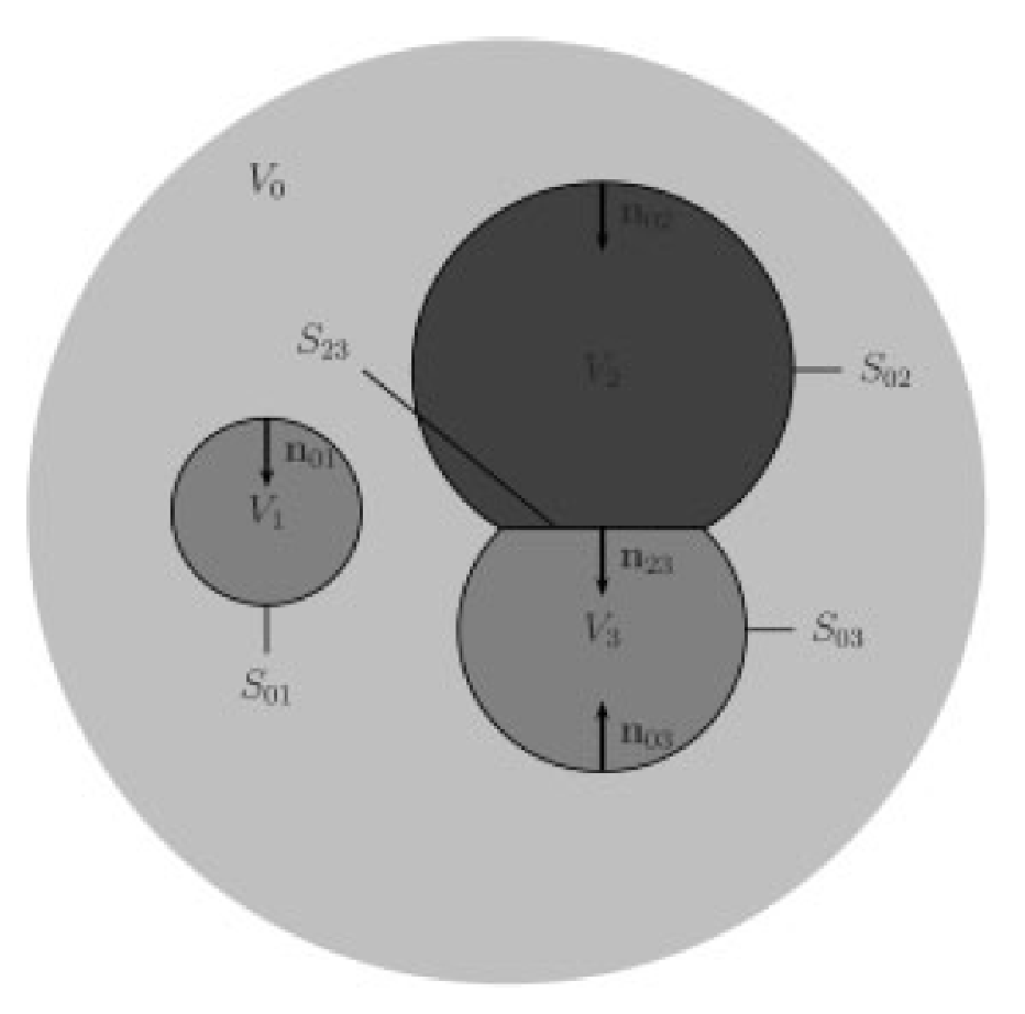
Then, we can transform the vector potential to obtain a contribution from both within each volume and from each surface
Here, the magnetization in the surface integral is evaluated just inside the volume , the primed sum excludes the term with , and is the outward normal from to on .
If the magnetization is uniform within , within and the volume integral vanishes. If the medium is uniform so is constant within , then within . In the magnetostatic case, the volume integral will again vanish.
If space is composed only of such regions
and the terms can be paired because and to give
where now is now evaluated just outside the volume . The quantity is the jump in magnetization as the boundary is crossed from to (in the direction of at the point .
The field follows immediately:
| (79) |
Alternatively, we may work from a similar version of the scalar potential:
Under the same conditions as before and the volume integrals vanish, leaving
The magnetic field is now given by
| (80) |
where is the appropriate magnetization at the point .
In this form it is easier to implement the boundary conditions when the materials are diamagnetic or paramagnetic. In either case, is the normal component of the magnetization at the boundary and
because Maxwell’s equations require the normal component of to be continuous across a boundary.
Hence,
| (81) |
This appears to be an equation that defines implicitly everywhere but it cannot be implemented as such because it does not define the discontinuous tangential component of fields on the surfaces . The general method of solution when everywhere is to solve Eq. [73] with vanishing right side:
| (82) |
This is Laplace’s equation, a version of Poisson’s equation without sources. Because there are no sources, the construction in Eq. [72] is not applicable and the solution of Laplace’s equation must be determined from the conditions imposed on the boundaries. The boundary conditions on at the surfaces between the different media are fully determined by the Maxwell equations, namely, that is continuous across the boundary so that the components of parallel to the boundary are continuous and the component of normal to the boundary is continuous, i.e., is continuous.
These prescriptions allow the magnetic field to be found exactly in all circumstances. In practice, however, the smallness of the susceptibilities allows approximations to be made that greatly simplify the estimation of the field. This is demonstrated in the illustrative example in the text above.
REFERENCES
- 1.
Brindle KM, Brown FF, Campbell ID, Grathwohl C, Kuchel PW. Application of spin echo nuclear magnetic resonance to whole cell systems: membrane transport. Biochem J 1979; 180:37–44.
- 2.
Endre ZH, Chapman BE, Kuchel PW. Cell volume dependence of 1H spin echo NMR signals in human erythrocyte suspensions: the influence of in-situ field gradients. Biochem Biophys Acta 1984; 803:137–144.
- 3.
Kirk K, Kuchel PW. The contribution of magnetic susceptibility effects to transmembrane chemical shift differences in the 31P NMR spectra of oxygenated erythrocyte suspensions. J Biol Chem 1989; 263:30–134.
- 4.
Matwiyoff NA, Gasparovic C, Mazurchuk R, Matwiyoff G. The line-shapes of the water proton resonances of red-blood-cells containing carbonyl hemoglobin, deoxyhemoglobin, and methemoglobin—implications for the interpretation of proton MRI at fields of 1.5-T and below. Magn Reson Imag 1990; 8:295–301.
- 5.
Chu SC-K, Xu Y, Balschi JA, Springer CS. Bulk magnetic- susceptibility shifts in NMR-studies of compartmentalized samples: use of paramagnetic reagents. Magn Reson Med 1990; 13:239–262.
- 6.
Levitt MH. Demagnetization field effects in two-dimensional solution NMR. Concepts Magn Reson 1996; 8:77–103.
- 7.
Jackson JD. Classical Electrodynamics, 3rd Ed. New York: John Wiley & Sons; 1999.
- 8.
Shadowitz A. The Electromagnetic Field. New York: Dover; 1975 (reprinted).
- 9.
Springer CS. Physicochemical principles influencing magnetopharmaceuticals. In: Gillies RJ, ed. NMR in Physiology and Biomedicine. San Diego: Academic Press; 1994. p 75–99.
- 10.
Lorentz HA. The Theory of Electrons and Its Applications to the Phenomena of Light and Radiant Heat, 2nd Ed. New York: Dover; 1915 (reprinted 1942).
- 11.
Feynman RP, Leighton RB, Sands M. The Feynman Lectures on Physics. London: Addison-Wesley; 1964.
- 12.
Dickinson WC. The time average magnetic field at the nucleus in nuclear magnetic resonance experiments. Phys Rev 1951; 81:717–731.
- 13.
Ramsey NF. Chemical effects in nuclear magnetic resonance and diamagnetic susceptibility. Phys Rev 1952; 86:243–246.
- 14.
Schey HM. Div, Grad and All That. New York: Norton; 1997.
- 15.
Russakoff G. A derivation of the macroscopic Maxwell equations. Am J Phys 1970; 38:1188–1195.
- 16.
Kuchel PW, Bulliman BT. Perturbation of homogeneous magnetic fields by isolated cells modelled as single and confocal spheroids: implications for magnetic resonance spectroscopy and imaging. NMR Biomed 1989; 2:151–160.
- 17.
Ramsey NF. Magnetic shielding of nuclei in molecules. Phys Rev 1950; 78:699–703.
- 18.
Wolber J, Cherubini A, Leach MO, Bifone A. Hyperpolarized 129Xe NMR as a probe for blood oxygenation. Magn Reson Med 2000; 43:491–496.