A nonadiabatic semi-classical method for dynamics of atoms in optical lattices
Abstract
We develop a semi-classical method to simulate the motion of atoms in a dissipative optical lattice. Our method treats the internal states of the atom quantum mechanically, including all nonadiabatic couplings, while position and momentum are treated as classical variables. We test our method in the one-dimensional case. Excellent agreement with fully quantum mechanical simulations is found. Our results are much more accurate than those of earlier semi-classical methods based on the adiabatic approximation.
pacs
32.80.PjOptical cooling of atoms; trapping and 03.65.SqSemiclassical theories and applications1 Introduction
One of the most spectacular achievements in the field of laser cooling is the discovery of cooling below the Doppler limit in optical lattices, so called Sisyphus cooling let88. An optical lattice is a standing wave of laser light, forming a periodic light-shift potential for atoms moving in the laser field jes96; gry01. In the optical lattices used for cooling the frequency of the lasers are tuned close to an atomic resonance. The atoms thus undergo cycles of absorption followed by spontaneous emission. Under the right experimental conditions, the spontaneous emission causes an overall loss of kinetic energy of the atoms, i.e., cooling.
Optical lattices are also widely used in Bose-Einstein condensation experiments blo05 and for quantum state manipulation mon02. These lattices are tuned far from atomic resonances, in order to avoid spontaneous emission which would destroy the coherence of the condensate. Therefore these far detuned lattices do not provide any cooling.
The name Sisyphus cooling comes from the first theoretical model for the process dal89; ung89. This model is based on optical pumping between the magnetic sublevels of the light shifted atomic ground state. However, at least in its original form it relies on a number of simplifying assumptions, such as a semi-classical approximation, spatial averaging, and a simplified level structure (a ground state with angular momentum , and an excited state with angular momentum ). Whereas this model correctly predicts some qualitative features of cooling in optical lattices, it is too crude to provide an overall quantitative agreement. Instead, a number of more advanced theoretical methods have been developed. The most accurate of these is the Monte-Carlo wavefunction technique cas95, a fully quantum mechanical method based on stochastic wavefunctions.
In this paper, we develop and test a new semi-classical method for simulating the motion of atoms in a near-resonant optical lattice. The most important approximation of our method is that the position and momentum of the atoms are treated as classical variables. Other approximations include a classical treatment of the light field, and adiabatic elimination of excited states of the atoms, but otherwise we make as few approximations as possible. In particular, the internal states are treated quantum mechanically, allowing for any kind of coherent superposition between magnetic sublevels.
Even though more exact fully quantum mechanical theoretical methods exist, semi-classical methods are valuable, partly because they are less demanding numerically, but also because they provide a simpler conceptual framework in which it is easier to formulate an intuitive picture of e.g. the mechanisms involved in the cooling process. Up to now, all semi-classical methods for laser cooling in optical lattices have been based on atoms that are pumped between definite internal states as they move through the lattice. To this end a basis of so-called adiabatic states, diagonalizing the light-shift potential at every position, has been used instead of the diabatic basis of the magnetic substates pet99. Coherences between adiabatic states have not been included in the description, and neither have so-called nonadiabatic couplings arising from the position dependence of the adiabatic basis. Thus, the motion of the atoms is described by purely classical equations, albeit the various potentials, pumping rates and diffusion coefficients have been derived from a quantum-mechanical origin. These adiabatic semi-classical methods reproduce some of the qualitative features of Sisyphus cooling, e.g. a linear relation between temperature and irradiance at high irradiances jer03. However, we show that even at very high irradiances the slope of this linear dependence does not agree with fully quantum-mechanical simulations. At the lower irradiances relevant to most experiments the adiabatic semi-classical method deviates even more severely from the fully quantum-mechanical results. Both these problems are solved by the nonadiabatic semi-classical approach.
2 Theory
In this section we develop the basic semi-classical equations of motion, on which our simulations are based. For generality the theory is developed in three dimensions. The angular momenta of the ground and excited states of the lattice transition are denoted by and respectively, and the corresponding magnetic quantum numbers are and . Although the derivation is more general, we shall in the end apply the theory to the case . Also, the light field creating the lattice could take different forms, but will in the end be assumed to have a linlin configuration in one, two or three dimensions gry01. That is, the lattice is created by the interference pattern of light fields, forming lattice sites with alternating and polarizations.
We start from the optical Bloch equations for an atom in a standing wave laser field coh90. They can be derived under very general conditions, and represent for practical purposes an exact fully quantum mechanical description of atomic motion in an optical lattice. Our first important approximation is that the population of the excited state is sufficiently low to allow its adiabatic elimination. The condition for this is that the saturation parameter
| (1) |
Here is the detuning from resonance, the natural width of the excited state, and is the Rabi frequency11 1 We use the Rabi frequency based on the total laser field. This is the same convention as was used, e.g., in Ref. pet99. Sometimes the Rabi frequency is instead on the laser irradiance per beam, which for a one-dimensional linlin configuration is half the total irradiance.. The details of the adiabatic elimination of the excited states can be found e.g. in Ref. coh90. This approximation is an important simplification, since it reduces the master equation for the full density matrix, to an equation for the density matrix of the ground states. The resulting equation for the evolution of reads
| (2) |
The first term on the right-hand side of this equation represents the Hamiltonian part of the evolution. The second term represents the non-Hermitian evolution due to spontaneous emission. The Hamiltonian contains the kinetic term and the light-shift potential,
| (3) |
where is the momentum operator of the atom, its position, , and the operator is given by
| (4) |
Here is an operator that promotes an atom from the ground to the excited state, while is responsible for the reverse process. In the basis of circular polarization vectors
| (5) |
they have simple expressions in terms of Clebsch-Gordan coefficients
| (6) |
In the basis of the magnetic substates the operator is represented a matrix .
For the simple model atom with and is a diagonal matrix. However, most atoms of interest have a more complicated level structure, including non-diagonal couplings in the potential. Therefore previous semi-classical methods have used an adiabatic basis, where the atomic states are the eigenstates of . Whereas is diagonal in the adiabatic basis, the position dependence of the basis gives rise to nonadiabatic couplings between adiabatic states. In the adiabatic approximation these couplings are neglected. In our method we keep all off-diagonal couplings. The results are then independent of the basis used, and the simplest choice is to stay with the magnetic levels , the diabatic basis. Since this basis is the same for all , all couplings are included in , and their functional form can be calculated analytically for a given laser configuration.
The second term on the right-hand side of Eq. (2) contains processes associated with spontaneous emission. Writing the matrix elements of in the position representation, , its form is
| (7) |
where . The matrices are given by
| (8) |
Hence, represents the excitation of an atom by the laser field, and its subsequent return to the ground state via spontaneous emission of a photon with polarization . The factors represent the atomic recoil from a spontaneously emitted photon with wave vector . The integration is over the directions of the emitted photon, and the summation is over any basis spanning the allowed polarization vectors. The recoil momentum of the atomic transition is .
Our goal is to approximate Eq. (2) by a semi-classical equation where every atom has a definite position and momentum, i.e. every atom follows a trajectory in phase space. This is of course not allowed in quantum mechanics, because of the uncertainty principle. Hence, a quantum mechanical phase space cannot be defined, but it is still possible to introduce a “coarse grained” version of phase space through the Wigner function
| (9) |
In this work the Wigner function is a matrix with dimension . The Wigner transformation of Eq. (2) becomes
| (10) |
Here and are the Fourier transforms
| (11) | ||||
| (12) |
No approximation has been made in going from Eq. (2) to Eq. (2), the Wigner transformation is just another representation of the same physics. Now, we introduce the semi-classical approximation. According to this approximation the momentum distribution varies smoothly and slowly over typical momentum transfers in Eq. (2). Since and have the same periodicity as the laser field, i.e. , Eqs. (11) and (12) show that the typical size for is the recoil momentum. Thus, the semi-classical approximation assumes that the momentum distribution changes little for emission/absorption of a single photon. As long as the atomic momenta are several recoil units large, and the effects of quantization of the atomic states are small, this approximation can be expected to work well.
Invoking the semi-classical approximation we can make a second-order Taylor expansion around of the Wigner distribution
| (13) |
Using this expansion it is possible to replace and by their counterparts in position space. The resulting equation for the semi-classical Wigner function, which now can be interpreted as a phase-space distribution, is
| (14) |
In this equation we use the short-hand notation , , where are the Cartesian coordinates. The constants come from the integration over the direction of the spontaneously emitted photon, and are given by
| (15) |
Although the equation is somewhat lengthy, it is possible to give physical interpretations to its terms. The left hand side is simply the kinetic term, i.e. the full derivative . On the right, the terms where appear without any derivative represent transfer of population between states, either by couplings from non-diagonal terms of the light-shift potential , or by optical pumping. The terms containing describe the motion of the atoms due to forces from light-shift potential and the radiation pressure. Terms containing second derivatives of both and first or second derivatives of or describe the momentum diffusion due to fluctuations in the number of photons absorbed. Finally, the term containing , but no other derivatives, contains the momentum diffusion due to the recoil kick from spontaneously emitted photons.
Equation (14) is the most complete semi-classical approximation for the time-dependent distributions of atoms in and space. It is classical in the sense that the atoms are assumed to be particles with definite positions and momenta. The internal states, however, are treated fully quantum mechanically, including all off-diagonal couplings and coherences. It is thus not possible to assign an atom to a definite internal state, nor is it described as a classical probability distribution over the different internal states, but as a quantum-mechanical superposition of internal states.
In order to solve Eq. (14) we recast it into a Langevin-type equation. That is, instead of calculating distributions of atoms, we shall calculate phase-space trajectories and of individual atoms. In doing this, we still want to keep the quantum mechanical description of the internal states. That is, the probability distribution of an atom is
| (16) |
Here is a matrix of dimension containing the internal-state density matrix of the atom at time . Inserting this form into Eq. (14), and integrating over position and momentum, the evolution equation for is obtained
| (17) |
Here and below, we use the simplified notation for and for . It is, however, important to understand that these are now time-dependent functions representing position and momentum of a single atom, which are conceptually very different from the variables in Eq. (14). Using that etc., we derive the equations for the evolution of and (see, e.g., risken)
| (18) | ||||
| (19) |
Here is a force and is a fluctuating force with the properties
| (20) |
The force is given by
| (21) |
The first term above is the force arising from the second-order light-shift potential, while the second term is the radiation pressure. The diffusion coefficient is
| (22) |
The first term arises from the recoil from photons spontaneously emitted in random directions, while the second term is connected to fluctuations in the radiation pressure. The latter term is in general anisotropic.
3 Numerical implementation
We simulate the equations (2), (18) and (19) in one dimension. The laser field has the form
| (23) |
At the start of every time step the system is in a pure quantum mechanical state. For every time step , , and are evolved using a second-order Runge-Kutta method. The fluctuating force is included as a term
| (24) |
where is a random number with zero average and unit variance. This term only needs to be evaluated once every time step hon92.
At the end of a time step, the system will not be in a pure state anymore. Its internal-state density matrix can, however, be decomposed into pure states
| (25) |
The coefficient are the eigenvalues, and the corresponding eigenvectors, of . Since is a density matrix, the eigenvalues satisfy the properties and , and can be interpreted as classical probabilities of the different states peres. Hence, at the end of each time step the system has the probability to make a “jump” into the pure state . Even though a density matrix in general has an infinite number of decompositions into pure states, the decomposition above is unique in the sense that it is the only one into a set of linearly independent pure states.
For numerical efficiency the eigenvalues were obtained using first-order perturbation theory, which is sufficiently exact if is short enough. In practice, one of the eigenvalues will be very close to one, while the others are small or zero. Thus, one can interpret the system as either staying in the same state, or jumping to a new state. When the eigenvalues obtained by perturbation theory indicate that the system makes a jump, the accuracy is increased by a full diagonalization of . The expense in computer time for this improvement is modest, since jumps are comparatively rare.
4 Results
In our simulations we used the parameters for the D2 line in cesium, i.e. , , and natural width MHz, and recoil energy J steck. The diagonal elements of the diabatic potential for this transition are displayed in Figure 1. We first investigated the steady-state momentum distributions. For potential depths the samples contained 5000 atoms, and were iterated for the time . To improve statistics the momentum distribution was averaged over the last of the evolution time. For low potential depths convergence is slower. Therefore we used 20000 atoms for , and the evolution time , with averaging over the last . For all runs the time step was , and the initial state a spatially uniform distribution with temperature of 10 K.

Results for as a function of potential depth for a detuning are displayed in Figure 2. Our results are compared to a full-quantum simulation using the Monte-Carlo wave function method cas95. The two methods are in excellent agreement. The relative difference is at most about 20%. It is not clear how much of this deviation can be attributed to the fundamental difference between the two methods, and how much is due to e.g. statistical uncertainties or other numerical errors. For deep potentials both methods give the same linear slope, although with a slight offset. The agreement continues all the way down through décrochage, i.e. the point where the curve turns around and starts to increase again for small potential depths, although statistical fluctuations in the full-quantum data make comparisons more difficult here.
It also evident from Figure 2 that the present method is a substantial improvement of the adiabatic method used in Ref. pet99. The methods do not even agree at large potential depths, where one would expect the nonadiabatic corrections to become small. Improving upon this method by including non-diagonal diffusion terms (for details see Ref. pet99) does not substantially change the situation. We note that even in the limit of vanishing nonadiabatic corrections our method differs from that in Ref. pet99 by allowing for coherences between the internal states. In the adiabatic basis the potential does not induce any coherences between internal states, but such coherences are still induced by optical pumping.

The semi-classical method also makes it possible to follow the motion of a single atom as it moves through the lattice. In Figures 3 and 4 we show the position, momentum, energy and internal state distribution as a function of time for a single atom in optical lattices with detunings , and potential depths and respectively. The energy was calculated as the sum of the kinetic energy and light-shift potential, i.e.,
| (26) |
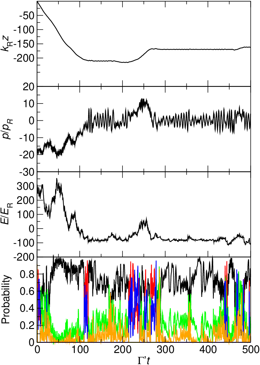
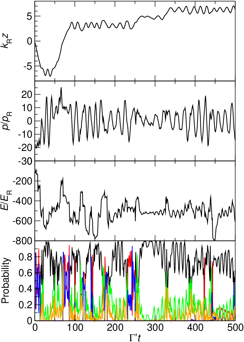
The ratio between the potential, pumping and diffusion terms in Eq. (14) depends on only, and is hence the same in both graphs. The only difference lies in the inertial term . Increasing , while keeping the ratio constant, is equivalent to increasing the mass by the same factor. This can be seen comparing the graphs, since the atom is less mobile in Figure 4.
At both potential depths the atom shows, after an initial cooling phase, a high degree of localization. While localized the atom populates mostly the extreme magnetic states . The energy is more or less constant, fluctuating around half the potential depth. The amplitudes of the oscillations in momentum and position vary somewhat due to diffusion, but tend to stay within certain bounds as long as the atom remains in the same potential well. We cannot see any clear trend towards smaller oscillation amplitudes while the atom remains trapped in a site, i.e., we see no local cooling.
The periods of localization are interrupted by brief phases where the atom acquires enough energy to travel over many potential wells, before once again getting localized. These excursions are most prominent at lower potential depths. The periods when the atom is untrapped are associated with abrupt changes of the internal state of the atom, usually from odd to even magnetic states. (The light-shift potential only induces odd–odd and even–even couplings between magnetic states. Thus any pure quantum mechanical state is a superposition of only odd or only even magnetic states.) During all periods of localization the atom is in a state with similar internal-state distribution and energy. Even when the energy sometimes drops below this stationary value the atom is soon returned to the same state.
These results are in qualitative agreement with our earlier conclusion that Sisyphus cooling, especially at low potential depths, works through a transfer of atoms between a hot and a cold mode cla05. The cold mode has a momentum distribution, with a width that does not change over time. This mode corresponds to the population of atoms in the trapped state. The cooling process is in effect a transfer of atoms from the untrapped to the trapped state.
In Fig. 5 we compare the semi-classical approximation to the time evolution of the momentum distribution (where is the number of atoms with momentum ) to the results in cla05, for . The bimodality of the distribution is very clear also in the semi-classical results, and the agreement with the quantum-mechanical results is very good. The distribution of the hot mode is identical to within statistical uncertainties. This shows that the physics of untrapped atoms, including their rate of transfer to trapped states, is well described by our semi-classical method. The semi-classical method gives a slightly more narrow cold mode, in agreement with the results in Fig. 2.

5 Discussion
We have developed a semi-classical method to simulate the dynamics of atoms in optical lattices. Our results for the average momentum distribution of the atoms, including its time dependence, agree excellently with those of the fully quantum mechanical method. To achieve an accurate description it is necessary to include both populations of and coherences between the internal states of the atom. The external degrees of freedom may, at least in some situations, be described classically, i.e., as particles with definite positions and momenta.
The semi-classical approximation was introduced as a second order Taylor expansion in of the Wigner function. According to our results , and hence this expansion should be a fairly good approximation. Nevertheless, there are some situations where the semi-classical description must necessarily break down. One is when effects from the quantization of bound states are important. Such effects will be most prominent when the atoms are localized near the bottom of the potential wells. Another is the coherent splitting of a wave packet. If the atomic wavefunction is, e.g., partially transmitted to the next potential well, the semi-classical method will describe this as a classical probability (some atoms are transmitted, some are not), while any coherence effects between the two parts of the wave packet will be lost.
The conceptual simplicity of the semi-classical descriptions makes it a useful aid in visualizing complex physical processes. It is also a flexible tool, which is relatively easy to adapt to different physical situations. In the near future we plan to extend the method to double optical lattices ell03. Further studies of the cooling process, e.g. to deepen the understanding of the bimodal velocity distributions observed in experiment and full quantum simulations, are underway.
Acknowledgments
We thank Robin Kaiser for useful discussions. This work was supported by the Swedish Research Council (VR), Carl Tryggers stiftelse, and Kempe stiftelserna. Part of the calculations were performed using the resources of the High Performance Computing Center North (HPC2N).
References
- (1) P. Lett, R. Watts, C. Westbrook, W. D. Phillips, P. Gould and H. Metcalf, Phys. Rev. Lett. 61, 169 (1988)
- (2) P. Jessen and I. Deutsch, Adv. At. Mol. Phys. 37, 95 (1996)
- (3) G. Grynberg and C. Robilliard, Phys. Rep. 355, 335 (2001)
- (4) I. Bloch, Nature Physics 1, 23 (2005)
- (5) C. Monroe, Nature 416, 238 (2002)
- (6) J. Dalibard and C. Cohen-Tannoudji, J. Opt. Soc. Am. B 6, 2023 (1989)
- (7) P. J. Ungar, D. S. Weiss, E. Riis, and S. Chu, J. Opt. Soc. Am. B 6, 2058 (1989)
- (8) J. Dalibard, Y. Castin and K. Mølmer, Phys. Rev. Lett. 68, 580 (1992)
- (9) K. I. Petsas, G. Grynberg, and J.-Y. Courtois, Eur. Phys. J. D 6, 29 (1999)
- (10) J. Jersblad, H. Ellman, L. Sanchez-Palencia, A. Kastberg, Eur. Phys. J. D 22, 333 (2003)
- (11) C. Cohen-Tannoudji, in Fundamental systems in Quantum Optics, Les Houches summer school of theoretical physics 1990, session LIII, edited by J. Dalibard, J. M. Raimond and J. Zinn-Justin (Elsevier Science Publishers, Amsterdam, 1992), p.1
- (12) H. Risken, The Fokker-Planck Equation, 2nd edn. (Springer, Berlin, 1996)
- (13) R. L. Honeycutt, Phys. Rev. A 45, 600 (1992)
- (14) A. Peres, Quantum Theory: Concepts and Methods, (Kluwer, Dordrecht, 1995)
- (15) D. A. Steck, Cesium D Line Data, http://steck.us/alkalidata
- (16) C. M. Dion, P. Sjölund, S. J. H. Petra, S. Jonsell and A. Kastberg, Europhys. Lett. 71, 369 (2005)
- (17) H. Ellmann, J. Jersblad and A. Kastberg, Phys. Rev. Lett. 90, 053001 (2003); H. Ellmann, J. Jersblad and A. Kastberg, Eur. Phys. J. D 22, 355 (2003)