The Spectrometer System for Measuring ZEUS Luminosity at HERAJournal: NIM in Physics Research, Section A
Abstract
The upgrade of the HERA accelerator has provided much increased collider luminosity. In turn, the improvements have necessitated a new design for the ZEUS luminosity measurements. The intense synchrotron radiation field, as well as the high probability of a bremsstrahlung photon in each bunch crossing, posed new experimental constraints. In this report, we describe how these challenges were met with the ZEUS luminosity spectrometer system. The design, testing and commissioning of the device are described, and the results from the initial operational experience are reported.
1 Introduction
ZEUS is one of two detectors accumulating data from electron-proton beam collisions at the HERA accelerator operated by the DESY laboratory in Hamburg, Germany. Analyses of such data have provided quantitative values of cross sections and derivative information related to the proton’s quark and gluon content, Quantum Chromodynamics, and other issues relevant to the Standard Model and beyond. In September 2000, HERA completed an eight year running period (HERA-I), which provided measurements of deep inelastic scattering (DIS), photoproduction, and other processes in a newly accessible kinematic regime. HERA underwent a luminosity upgrade in 2001 [1]. The goal was to increase the HERA-I peak luminosity by a factor of 5. In addition to the accelerator modifications necessary to achieve this, spin rotators were installed to provide electron beam longitudinal polarization of about on average. A new physics program (HERA-II) began in 2002 to make accurate measurements of small cross sections with polarized beams.
Precise knowledge of the luminosity is required for precise determination of a cross section associated with any process; such measurements depend on luminosity integrated over time, , to normalize the numbers of events observed during the same time period. Luminosity had been measured [2, 3, 4] in HERA-I using the rate of high energy photons from the bremsstrahlung process, , produced by the colliding beams. This process is well understood, has a high rate and an accurately calculable cross section. Produced photons follow the direction of the colliding beam electrons and are observed about 100 m downstream, after the electron and proton beams have been magnetically separated. The ZEUS HERA-I technique, with a calorimeter to directly measure all bremsstrahlung photons faces new difficulties at HERA-II, including the following:
- •
A significant increase in direct synchrotron radiation (SR) flux from the electron beam occurs due to the higher beam currents and to a new beam focusing scheme to optimize high luminosity near the interaction region.
- •
Much larger numbers of overlaid bremsstrahlung events (pile-up) occur. Colliding bunches producing more than one photon are not separated in the calorimeter technique. HERA-II luminosity implies a significant probability (approaching unity) for several final state photons with GeV in each bunch-crossing.
- •
There are additional requirements for accurate cross sections using polarized beam electrons (or positrons).
The HERA beams each consist of 220 bunches separated by 96 ns. A few bunches are unfilled; the empty bunches are used for monitoring purposes and they are also needed for the proton beam abort system, and the unpaired bunches are used to measure small backgrounds resulting from the electron or proton beam interacting with residual gas near the intersection region. After acceleration, the polarization of the electron beam [5] rises from to over a period of about minutes and the beam polarization might be different for each bunch. Therefore, the luminosity must be measured accurately for bunch over time intervals much less than . In addition, a fast luminosity measurement is essential for obtaining collisions, and monitoring and optimizing luminosity during a fill.
The required accuracy in the luminosity measurement for HERA-II is , which is similar to the most accurate luminosity measurement achieved at HERA-I. The luminosity spectrometer described in this paper utilizes a new method of measuring luminosity at ZEUS which addresses the new problems of synchrotron flux, pile-up, and other requirements, while meeting the specifications for luminosity accuracy required by ZEUS physics goals.
In the spectrometer system, the bremsstrahlung photons are detected through their well understood pair conversion, , in material of a beam-pipe exit window well downstream of the interaction region where these photons have been spatially separated from the circulating beams. After the converted electron pair 11 1 In this paper, ”electron” is meant to specify both electron or positron. Note that, aside from the direction of bend in the field, their interactions are identical at these energies. has been spatially split by the magnetic field of a dipole magnet, the particles are individually detected by two small electromagnetic calorimeters placed at transverse distances separated from the direct synchrotron radiation and unconverted bremsstrahlung beams. The observed rate of converted photons is proportional to the luminosity, as described in Sec. 4.
This setup reduces dramatically the requirements on data rate for the spectrometer calorimeters, since the primary photon beam bypasses them and the magnet insures that the large flux of low energy electrons from synchrotron photon conversions in material upstream of the magnet are swept away from the detectors. Due to the small conversion fraction () in the window and the limited accepted energy range, the pile-up problem is reduced by two orders of magnitude, so that multiple observed photons constitute only a few percent of the rate even at the highest luminosities expected for HERA-II.
With the relaxed rate requirements on the spectrometer calorimeters, their design can be sophisticated enough to simultaneously provide relatively precise measurements of the converted electron energies and positions — in turn giving similarly precise information for the bremsstrahlung photon. The redundancy and precision of the measurements provide important assurance on many aspects of the acceptance which must be known accurately with this technique. In general, the technique is simple and accurate, and works well at high luminosities.
The structure of this paper is as follows: in Sec. 2 are presented the details of the design of the luminosity spectrometer, including the calorimeter modules and a brief description of the data acquisition system. The detector calibration in a momentum analyzed electron test beam, and the reconstruction of photon properties from the calorimeter measurements are described in Sec. 3. The method of calculating the luminosity is described in Sec. 4, and the calibration and operating performance during the first months of HERA-II operation are presented in Sec. 5.
2 Spectrometer design and components
A schematic layout of the spectrometer system is shown in Fig. 1. The coordinate system is defined with the positive -axis along the photon beam direction, pointing upwards and along the line away from the center of the HERA ring. Here we describe each component in the order encountered by a photon, beginning at the exit window of the photon beam pipe, through the collimators, magnet, and the calorimeters. Relevant aspects of the data acquisition system are also described.

The bremsstrahlung photons from the intersection region travel through a long vacuum pipe terminating at an exit window, at 92 m from the nominal intersection point (IP). Upstream of the window inside the vacuum chamber (not shown in Fig. 1) are various aperture restrictions such as collimators, magnets, and other apparatus. Figure 2 shows the picture of a foil sensitive to synchrotron radiation, which was located in the beamline near the front face of the calorimeters. The foil clearly indicates the aperture delimited by upstream obstacles. For scale, the maximum horizontal extent of the aperture is 9 cm. The maximum vertical limits are representative of the 7 cm aperture of the fixed collimator.

The window, at the upstream end of the spectrometer system, terminates the vacuum so that the remainder of the detection system is in air. Approximately of the photons convert into pairs in the window. The typical energy of photons of interest is about GeV. The distributions in and photon impact positions at the window within the acceptance region reflect primarily the angular divergence of the primary beam electrons as they collide in the upstream ZEUS interaction region.
The converted electron pairs that successfully traverse subsequent collimators closely follow the original photon direction, until they encounter the magnetic dipole where they are split vertically. The magnetic field is such that a typical 10 GeV electron (positron) will then travel in the directions with a vertical angle of about rad, and encounter the calorimeters, whose vertical midpoints are displaced approximately cm from the incident photon beam. The calorimeter modules permit measurements of the electrons’ and positions with resolution of about 1.0 mm, and energies with resolution of about at 10 GeV. Calibrations in an electron test beam (described in Sec. 3) and in operation with the spectrometer (described in Sec. 5) verify these calorimeter measurement precisions.
Events with electrons detected in both calorimeter modules are used to reconstruct the original photon’s energy and transverse coordinates. The measured coincidence rate permits calculation of luminosity, as described in Sec. 4. The bremsstrahlung position distributions, while relevant to luminosity calculations, also provide a diagnostic of the interaction region for HERA operation.
The locations of the different spectrometer elements were obtained from optical survey and verified with beam data. Transverse distances are known to a precision of order 1 mm while the dimensions along the direction of the beam are known with a precision of better than 1 cm. These accuracies satisfy the requirements for the luminosity measurement.
2.1 Exit window
The composition of the exit window is shown in Tab. 1:
| Material | Percent by Weight |
|---|---|
| Aluminum | 85.3 |
| Silicon | 10.9 |
| Iron | 0.3 |
| Copper | 2.7 |
| Magnesium | 0.3 |
The diameter of the window is 100 mm. The window thickness was measured at several positions; the average thickness was mm with an RMS of 0.0054 mm, implying at least that level of uniformity. The fraction of converted photons in the window is therefore also uniform over the surface of the window. The variation in the cross section for photon energies between 5 GeV and 20 GeV is [6]; within the narrower energy window used for luminosity measurements, the energy dependence is very small and well simulated.
The radiation length of the exit window alloy is cm, which means that the exit window itself represents , so that about of interesting photons convert in the window. Converted electrons traveling through the material may subsequently radiate and lose a fraction of their energy. This effect is small, well understood, and simulated accurately. Also simulated is the multiple scattering of converted electrons, which leads to typical RMS deflections of rad and a transverse spread at the calorimeter front surface of mm. The resolution of reconstructed photon conversion positions is dominated by this multiple scattering of electrons in the window.
2.2 Collimators
The collimators are used to select observed photons within a rectangular region inside the transverse dimensions of the vacuum pipe and within the uniform field region of the magnetic field.
The fixed collimator is a block of stainless steel, 30 cm long, with internal aperture . It shields the calorimeters and the magnet from exposure to direct bremsstrahlung or synchrotron radiation photons from the circulating electron beam. However, measurements from synchrotron radiation indicate that beam elements upstream of the exit window more stringently limit the photon aperture, as shown in Fig. 2 and verified with bremsstrahlung measurements described in Sec. 4.
The moving (slit) collimator is a 15 cm long, water-cooled block of copper. When inserted, it restricts bremsstrahlung photons to pass through a narrow () slit 22 2 The height was optimized for high rate while maintaining small edge effects.. During normal running conditions, the moving collimator is out of the beam. When inserted it allows precise calibration of the absolute energy scale of the calorimeter channels (see Sec. 5).
2.3 Dipole magnet
The spectrometer uses a 60 cm long dipole magnet with a 10 cm horizontal aperture and typical field strength of T. The bottom of the proton beam pipe passes only a few centimeters above the top of the bremsstrahlung aperture and the effect of the dipole field on proton beam operation must be minimal. Hence magnetic shielding is arranged in the vicinity of the magnet around the proton beam-pipe. The shielding is a cylinder of diameter 85 mm, and centered at mm, mm with respect to our coordinate system (and the center of the magnet).

The magnetic field was measured, using a Hall probe, as a function of position at several different magnet currents [7]. The integrated magnetic field in the central region versus excitation current, shown in Fig. 3, indicates that the field is linear over the range of normal operation, and saturates slightly at the highest excitation currents used. The position dependent measurements have been interpolated using Maxwell’s equations supplemented with a Jacobi relaxation method to obtain the full and continuous magnetic field map. This map was implemented in the simulation program. The systematic errors have been estimated using the OPERA program [8, 9]; the differences are shown in Fig. 4 over a region which encompasses the full transverse aperture. Uncertainties thus estimated were typically less than throughout the acceptance region encompassed within mm, with an average uncertainty less than near the region of highest flux. Therefore, the magnetic field is well understood and creates an even smaller uncertainty on the precision of the luminosity measurement.

2.4 Calorimeters
The two calorimeter modules were originally constructed as “Beam pipe calorimeters” (BPCs) in ZEUS to measure DIS processes at very low values of [10]. They were designed to measure positions and energies of electrons near the HERA beam energy (27.5 GeV). The original description of their construction can be found in [11, 12]. For this application, one module was rebuilt in order to fit within the space constraints. The main parameters are listed in the Tab. 2 and the relevant properties and changes are elaborated here.
| Calorimeter Specifications | |
|---|---|
| Depth | |
| Moliere radius | 13mm |
| Energy resolution (stochastic term) | |
| Energy scale calibration precision | |
| Energy uniformity | |
| Linearity | |
| Position resolution | mm |
Both BPC modules are segmented tungsten-scintillator sampling calorimeters, permitting simultaneous measurement of the electron’s energy and transverse position of impact. The passive layers contain 26 plates of 3.5 mm thick tungsten alloy. These 24 electromagnetic radiation lengths () are more than adequate for longitudinal containment in this application. The active elements consist of scintillator fingers, alternating after each plate in the and directions, each finger 7.9 mm wide and 2.6 mm thick. One end of each finger is aluminized to provide an efficient end reflector. Each scintillator is optically decoupled from its neighbors by a wrapping of aluminum foil. The net effective width of each finger, including wrapping and air gaps, is 8.0 mm.
The other end of each scintillator finger rests against a wavelength shifting (WLS) bar 7 mm wide and 2 mm thick. The scintillator fingers oriented in alternate layers, in the longitudinal direction, are observed with one WLS bar representing a single readout channel. Each bar is viewed by a photomultiplier (PMT) from the rear. The WLS is aluminized at the front end to reduce attenuation effects. To compensate for remaining attenuation in the WLS bars, they were wrapped in reflective correction masks to ensure longitudinally uniform response from each scintillator located along the length of a bar. The geometry of some WLS bars required redesign for this application; they were bent and pointed toward the new locations of the Hamamatsu R5600U-03 PMTs [13].
Each module has 16 channels for -position reconstruction. For the -position, the lower module has 15 channels and the upper 11 channels, reflecting limitations imposed by the small separation between the photon beam and the proton beam pipe. The 84 mm transverse separation of the modules is maintained by rigid brass bars. Since the calorimeter containment vessels incorporate 5 mm of tungsten on surfaces adjacent to the beam, the net transverse distance between inner scintillators of the two modules is 94 mm. These positions and the trajectories of electrons after traversal of the magnetic field are discussed more fully in Sec. 3.
In order to protect the calorimeters from radiation due to scattered synchrotron radiation, the unconstrained sides and rear were shielded by bricks and sheets made of lead. Also, a thin (5 mm) sheet of lead was placed in front of the modules. A system of light emitting diodes (LEDs) provides fast light pulses to all PMTs of a module simultaneously under remote command. This system permits the relative PMT gains to be monitored for short term changes. The LED system also provided an independent monitor of deadtime effects.
The relative channel-to-channel gains were initially set using test beam electrons, described in Sec. 3. The relative response of each channel was monitored with calibration runs as described in Sec. 5. The calibration runs were important, especially during early running when unstable beam operation created changes in channel-to-channel response. (These were found to primarily arise from irradiation of WLSs near the PMTs.) Changes were monitored and compensated to maintain the relative gains of all readout channels within a module as well as the relative average gains of the two modules.
2.5 Data Acquisition System
One important challenge in this application is accurate digitization of the calorimeter PMT signals, which are separated by the 96 ns HERA bunch spacing. In order to minimize noise, analog processors were located in the HERA tunnel close to the detectors. These electronics are inaccessible during normal HERA running. The digital electronics is accessible, located in the ZEUS main hall about 100 m upstream of the luminosity detectors. The spectrometer data acquisition system (DAQ) was designed and constructed by the ZEUS Krakow group [14] and DESY electronics development group, and is common to the luminosity calorimeter system and the 6 meter tagger[15]. The latter system records the energies of final state bremsstrahlung electrons with energies complementary to those accepted by the spectrometer.
Figure 5 outlines the full system. The digitized signal is used immediately in the triggering system and retained for the luminosity calculation. In more detail, the readout system consists of the following components:
- •
The front-end electronics (FEE) is the analog system of amplifiers and drivers used to shape and transmit the analog PMT signals to the digital system.
- •
The digital electronics includes eight flash analog-to-digital converter (FADC) boards, four memory boards (MB), and one trigger board (TB). Each MB performs operations on the data as well as storage. All are located in a single VME crate.
- •
A PC, operating under LINUX, for online processing of the data and calculation of the ZEUS luminosity.

The signal from each PMT is transferred through a 6 m long cable to the FEE crates. The FEE amplify and shape these signals and drive them through the 135 m long RG213 transmission lines to the digitization units in the ZEUS hall. Additionally, the FEE crates each contain driver modules for an LED (input to the PMT cathodes) and charge-injector to the FEE amplifiers. These can be independently triggered to test both the PMTs and the remainder of the DAQ system. The analog signals are integrated with a time constant of 65 ns and subsequently digitized by 12-bit FADC modules operating at about 10 MHz, synchronously with the HERA beam bunches. Each FADC board consists of a pole-zero filter, which shapes the input analog signal to reduce the decay tail. Digitized values from each PMT for each bunch crossing are transferred to the 16-channel MBs residing in the same VME crate. The MB performs the following operations on each signal:
- •
A subtraction is made of the stored digital value from the previous bunch crossing to provide a dynamic pedestal subtraction. In the process, low frequency noise (compared to 10 MHz) is removed. The low rates in all channels of the spectrometer ensure few mistakes due to signals in consecutive bunches.
- •
Sums are made of all the channels in each dimension of the upper (, ) and lower (, ) calorimeters, resulting in four energy sums (, , , ) in each crossing contained in the four MBs. These sums are retained with the signals from the individual channels. The sums are also sent to the TB where they are used for triggering decisions (data retention) on each beam crossing.
- •
Meanwhile the data have been placed in a buffer to await the trigger decision. For events in which the TB flags the event as useful, the data are copied sequentially to output buffers. These buffers are read continuously via VME at a rate up to 10 kHz.
The TB, in the VME crate with the MBs, communicates with the MBs through a custom backplane. The programmable TB decides when an event satisfies specified criteria; if so, it sets an ACCEPT signal on the backplane. The criteria utilize two digital sums: one () from all the and channels; the other from the corresponding sum () in the down detector. Only events that pass a nominal threshold value in each of the two detectors are passed on for further consideration.
If the MB buffer were to become full, data acquisition must halt until buffer space is available. This is a situation requiring deadtime corrections, which are best minimized. Therefore, at the highest luminosities, a trigger prescale factor is applied to maintain an average rate well below the maximum trigger rate of 10 kHz. The TB provides counters that record (1) the total number of HERA bunches and (2) the number in which the MB buffer is not full and active. When the MB buffer is full and incoming data must be discarded, the active-time counter stops counting. These counter values, sent to the online PC each second, provide a continuous deadtime correction for the luminosity calculation and also permit this deadtime to be monitored. The deadtime correction and the prescale factor are independently measured using light test events by recording both the LED signal rate and the rate at which these events are recorded. The prescale factor was set to 3 during HERA high luminosity running.
Data from accepted events are transferred to output MB buffers and sent via VME bus to the online PC. The information is used to reconstruct the energy and position information for the detected photon, as described in Sec 3, and is stored in histograms for monitoring purposes. The ZEUS luminosity is calculated offline using histograms and counters saved to tape every 16 seconds, as described in Sec. 4.
3 Calorimeter Reconstruction of Electrons and Photons
3.1 Reconstructing electron energies and positions
The functions of the calorimeter modules are to measure the energies and transverse coordinates of the two electrons, respectively in the up () and down () calorimeters, using the information recorded from the PMT channels associated with the horizontal and vertical strips. The calorimeters were extensively tested in a DESY-II electron beam at energies up to 6 GeV, prior to installation in the HERA tunnel. Described here are the algorithms used to transform the charges recorded by the PMTs into the incident electron energy (energy calibration) and the transverse position coordinates, as well as the tests performed in the electron test beam. The measurements show that the calibration precision is more than adequate for the present task. The position and energy resolutions, leakage effects, as well as remaining attenuation in the scintillator strips were also measured with the test beam. The measured leakage and attenuation effects with test beam have been used to correct the energy reconstruction of data. Further calibration checks on the modules were performed in the spectrometer configuration, as described in Sec. 5, in order to maintain the calibration during operation.
The preliminary settings of the PMT gains were set using an LED system. Also, by varying the high voltages applied to the PMTs, an empirical function was obtained providing the relative gain variation with high voltage, independently for each channel. Additional tests, including absolute calibrations, were carried out in the test beam.
The test beam setup located each module on a movable table, which could be translated horizontally and vertically by known amounts with a stepping motor. The electron test beam was focused, steered, and momentum defined by magnetic beam elements. Counters constrained the beam to be within a transverse circle of 3.0 mm diameter. Initially, the module was located with the 5.0 GeV beam incident near its center. The gains of the PMTs were set to nominal values, and the resulting net charge (in ADC counts) from each PMT channel was recorded for each event as the module was scanned horizontally or vertically. Using these scans, the PMT gains were then adjusted, by changing the applied voltage according to the empirical functions previously measured, so that the peak charge was the same for all channels. This procedure converged after a single iteration.
Figure 6 shows typical data (points) from four adjacent channels in such a horizontal scan. The points joined by a continuous curve represent a single channel’s response. Recalling that an individual scintillator width is 8.0 mm, the figure also illustrates that electron showers typically deposit a substantial fraction of their energy in at least two channels, but very little energy is outside four channels.

By repeating such horizontal scans at different vertical positions, any uncompensated light attenuation in the scintillator was measured so its effects could be corrected during analysis. The overall gains were set so that the total energies for electrons incident at the midpoint of the module from the horizontal and vertical channels were equal. From the known beam energy, the charge response was calibrated directly to the sampled energy as a parameter for the channel as energy divided by average recorded charge. These parameters were then used to reconstruct shower energy as described below.
To minimize noise, only strips near the shower maximum were actually used for reconstruction. The energy of the incident electron sampled from the -strip sum is
| (1) |
where the sum runs over a cluster of the four highest energy adjacent strips; is the charge from the channel (in ADC counts), corrects for transverse energy leakage (a small effect except at the edges of the calorimeter) and corrects for the small residual attenuation as measured in the test beam. The positions () of the shower centroid were also obtained from the event, as described below. The measurement of , the energy sample of the -strips, was obtained in a similar manner.
The total energy of the electron was
| (2) |
The position coordinates were calculated using linear energy-weighted means over the deposited energy. For the upper calorimeter, the internal -coordinate for the shower, , was obtained from 33 3 A logarithm weighted algorithm though slightly more precise was not used here because it was found to be too time consuming for the online processing, and it is not well described by the simulation.
| (3) |
where is the known central location of the channel strip within the calorimeter. Only channels above a threshold energy of 60 MeV were used for these sums. The position in the spectrometer coordinate system for the electron in the up detector, is given by
| (4) |
where is the known alignment offset relative to the coordinate system of Fig. 1 for this calorimeter. The shower -coordinate, , was obtained similarly.
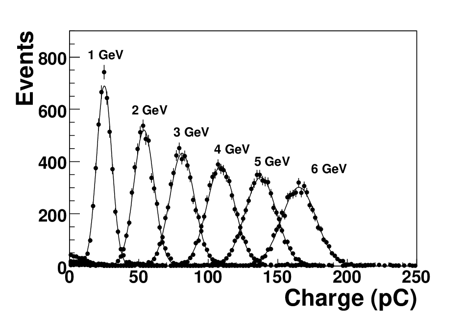
The reconstructed energy response was measured with differing known test beam energies; the spectra for six different energies are shown in Fig. 7 and illustrate that the measurements show the expected results. Figure 8, showing the mean response as a function of the beam energy, demonstrates that the response is linear up to at least 6 GeV. The intrinsic linearity of calorimetry and the tested linearity of the electronics implies linearity for even higher energies.
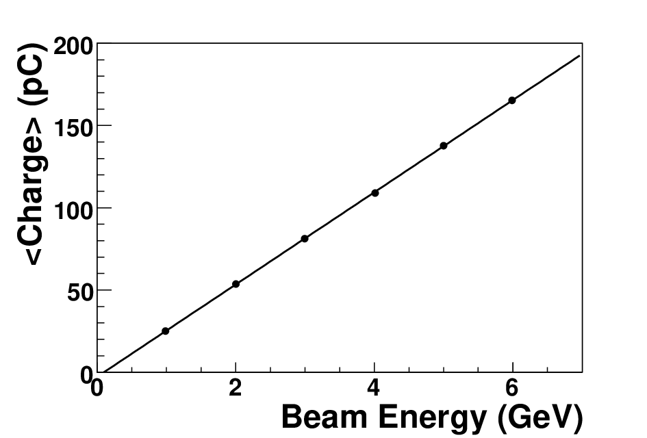
Figure 9 depicts the RMS deviation from the mean as a function of energy: the parameterization indicates that in the region of intended measurement, around 9 GeV, the RMS is mainly proportional to the stochastic term, as expected for a sampling calorimeter.

3.2 Reconstructing bremsstrahlung energy and position
The operation of the calorimeter modules in the bremsstrahlung beam is discussed in detail in Sec. 5. We note that, in this geometry where the and calorimeters measure the two electrons, the original photon may be directly reconstructed from these measurements. The energy of the photon is
| (5) |
The transverse -position of the photon is
| (6) |
and the transverse -position (bend plane of magnet) is
| (7) |
The energy weighting in the last equation arises because the magnet imparts equal transverse momentum to each electron.
4 Luminosity Calculation
Colliding beam luminosity is quantitatively related to the circulating beam currents and the spatial overlap as they intersect. By definition, the integrated luminosity in the collision region provides the normalization for any cross section so that, if events of a specific process are observed during the time period during which the integrated luminosity is known, then the cross section for that process is
| (8) |
where is typically specified in units of inverse picobarns .
4.1 Instantaneous and specific luminosities
The instantaneous luminosity () is defined, for the purposes of this paper, to be the luminosity averaged over the period between accelerator bunch crossings (96 ns). Since scales with the product of the electron () and proton () currents, it is convenient to define the specific instantaneous luminosity
| (9) |
where the sum includes the currents in all colliding bunches.
4.2 Luminosity Measurement

The most accurate method for measuring luminosity is to measure the rate from a process whose cross section is large and well known. At HERA, luminosity is calculated from the measured rate, , of photons created in the bremsstrahlung process . The energy spectrum of bremsstrahlung photons is accurately described by the Bethe-Heitler formula [16], shown in Fig. 10 as the product of energy and differential cross section, in millibarns, as a function of photon energy. Additional corrections from radiative processes affecting the spectrum at energies above 5 GeV are well understood and incorporated into calculated cross sections. The photons of interest here are those whose converted electrons have energies appropriate to enter and trigger both calorimeter modules. As discussed below, the nominal magnetic field and geometry are such that the photon energies of interest are typically near 20 GeV.
Luminosity is obtained from the equation
| (10) |
where is the bremsstrahlung cross section integrated over the same energy interval as the measurement of . The parameter, , represents the fraction of photons in the bremsstrahlung beam that convert into electron pairs in the material upstream of the magnet, primarily in the exit window. The acceptance, , includes the overall probability (not included in ) for a photon created at the intersection region to be observed as an pair in the spectrometer. Imprecise knowledge of creates the largest uncertainty in the measurement, as will be discussed in detail below. The acceptance of the luminosity system depends primarily on two issues:
- •
obstacles upstream of the entry to the luminosity system that remove photons from the edges of the bremsstrahlung beam;
- •
the fraction of the converted pairs in which both electrons are accepted into the fiducial areas of the calorimeters.
The conversion fraction and these two contributions to the acceptance will be discussed in turn.
4.3 Conversion fraction, f

The fraction of photons converted into pairs depends on (a) the absolute and energy-dependent pair production cross section and (b) the details of the conversion material in the exit window and the air between the exit window and the magnet. 44 4 The gas in the entire vacuum pipe upstream of the exit window is negligible. The materials and thickness of the exit window are well understood, and described in detail in Sec. 2. The total pair production cross section on each nucleus is largely independent of photon energy and is given to good accuracy by a simple formula that depends on the radiation length and other well-understood properties of the converting material. The differential cross section for one electron of the pair to retain a fraction, , of the photon energy, shown in Fig. 11, is also largely independent of energy.
The conversion efficiency and acceptance used in this analysis were calculated using the full GEANT 3.21 simulation. Subsequent propagation and interactions of the electrons used the fully parameterized magnetic field map discussed in Sec. 2.
4.4 Upstream Obstacles
The acceptance includes a correction for incoming photons obscured by upstream obstacles. The unobscured region was delineated in two independent ways: (a) the aperture obtained from a foil sensitive to synchrotron radiation described in Sec. 2; and (b) measurements of the transverse tails of the bremsstrahlung beam obtained by moving its centroid across the aperture. The two methods agree in detail as shown in Fig. 12, where the sharp contour delineates the region indicated by illumination of the foil shown in Fig. 2. The elliptical contours show regions observed from bremsstrahlung photons due to beam collisions at the intersection region as the electron beam was steered through various incident angles. The regions from the bremsstrahlung runs in Fig. 12 can be seen to outline the same aperture as that indicated from synchrotron radiation.

With beams steered in their nominal directions, Fig. 13 shows a typical measurement of the contours due to bremsstrahlung produced by the intersecting beams. Note that the intersecting beam profile has a clear elliptical shape, wider in the horizontal than the vertical. The major axis of the ellipse is seen to be rotated around the beam direction. The detailed shape was found to fit orthogonal Gaussians at axes rotated by about 10 degrees to the horizontal. Typical distributions, projected along the orthogonal rotated axes, had standard deviations about 2 cm along the more horizontal axis and 1 cm along the more vertical axis. The fitted 1D distributions are discussed further in Sec. 5.

The acceptance correction for the photons blocked by the upstream aperture typically amounted to , depending primarily on the photon beam properties at the time.
4.5 Converted Pairs Accepted into Calorimeter
The spectrometer acceptance depends on the fraction of photons converted upstream of the magnet for which electrons of the pair enter the calorimeters. This acceptance depends strongly on the distribution in shown in Fig. 11 and on the energy of the interacting photons, , because of the deflection of each electron by the magnetic field.
Most of the acceptance dependence on and can be understood from elementary arguments. Consider photons traveling along a beam axis transversely located midway between the calorimeter modules with 55 5 The actual vertical coordinate origin described here is offset about 0.5 cm in our system. (See Figs. 1 and 18.) A hypothetical simplified case is used here for pedagogical reasons.. Each electron acquires the same transverse momentum, in opposite directions, from the field traversal: , where the integral represents the integrated magnetic field (in Tm) along the path through the magnet. At the nominal running current (225 A), the value of GeV. The deflection of an electron of momentum (in GeV/c) in the magnetic field can be approximated as
| (11) |
where is the distance from the center of the magnet to the calorimeters. Only when the values of for each electron are such that both enter “good” calorimeter regions are events accepted. If the fraction of the photon energy acquired by the upwardly deflected electron is , the other electron acquires a fraction of the photon energy. It follows that and are directly related to the electrons’ locations. The locations of the electrons in the upper () and lower () calorimeter modules are related to and as follows:
| (12) |
The inner and outer -limits of the fiducial areas of the two calorimeters therefore delineate limits in the plane of versus that are accepted. This is illustrated in Fig. 14, where the limits due to the outer and inner -limits of the upper and lower calorimeter modules define the accepted region to be that internal to the curves.

If all photons arrived with coordinate , the acceptance at fixed would be the integral of the function in Fig. 11 over the accepted -range shown cross-hatched in Fig. 14. This simple acceptance function is shown as the solid line in Fig. 15. The result of a more detailed Monte Carlo calculation for this beam configuration, the points in the same figure, shows that this simple model gives the major features of the acceptance. Note that the coincidence requirement of two electrons without any restriction on energy provides an acceptance approximating that shown in Fig. 15. This description, as discussed more fully in Sec. 5, permits luminosity to be measured which only indirectly depends on energy calibration. At the same time, consistent comparisons of the relevant data distributions with predictions validate the calibration.
The actual acceptance, however, varies slightly from the curve shown in Fig. 15 because the photon beam’s finite extent in creates complications. Photons displaced from the beam centroid shifts the contours in Fig. 14 by amounts of order for each centimeter of -displacement. In addition, though the calorimeters sample the full transverse range of the transmitted beam, the correlations between vertical beam coordinate, photon energy, and acceptance require that we address the beam properties in the acceptance calculations. Full acceptance calculations include the entire spectrometer setup, the measured beam shape, and the complete shower development in the calorimeters as described in Sec. 5.

4.6 Small Corrections and Uncertainties
The magnet current was chosen so that, during normal operation, the data cover the flat part of the bremsstrahlung energy spectrum in Fig. 10. This ensures that the sensitivities to energy scales and alignments are minimized. Certain additional, small corrections were included, as described here.
The measured rate requires correction for backgrounds from electron beam interactions with the residual gas in the beam pipe. This is determined by utilizing the measured coincidence rates corresponding to pilot bunches with electrons unpaired with proton bunches. For typical running conditions this effect on the luminosity measurement is , and the uncertainty is much less. Proton beam related backgrounds are negligible. Correction for multiple photons observed in a single bunch crossing is also negligible. The overall precision of the luminosity measurement is discussed more fully in Sec. 5
5 System Operation
Luminosity measurements provided by the spectrometer system utilize spectra of the bremsstrahlung photon position and energy from the calorimeters. procedures allowed for continuous validation of the precisions for these quantities. Specifying accurately (a) the axes of the beam coordinate system relative to the calorimeter modules; and (b) the relative and absolute energy measurements by the calorimeters were necessary in circumstances in which these changed over time. These issues are discussed in turn.
5.1 Position Measurements
The photon position is derived directly from the measurements of the individual electrons as specified in Eqns. 6 and 7. Measurements in the two transverse directions have somewhat different precisions.
Because electrons are deflected by the magnetic field primarily in the vertical plane, the horizontal positions in the upper and lower calorimeters should be nearly equal. The average (Eqn. 6) is used to estimate the value of . Fig. 16 shows the complementary difference between up and down measurements . The expected mean of this quantity should be nearly zero and the standard deviation should be similar to the error on . The observed RMS of about 3 mm is close to the anticipated value, and is dominated by the scattering of the electrons in the exit window. The small offset of the mean is attributed to uncorrected vertical components of the magnetic field and a small horizontal misalignment of the calorimeter modules.

Figure 17, the spectrum of reconstructed coordinates obtained with the 2 mm high slit collimator inserted, provides a rough estimate of the RMS for measurements of . Note that this measurement is compromised by the correlations with the energy measurement reflected in Eqn. 7, but also by the finite width of the slit, and by scattering from the slit edges. Hence, the RMS of 7 mm should be considered an upper limit on the actual precision on . The edge scattering also is known to produce the tails in the distribution of Fig. 17.

Because the calibration of the calorimeter energy scale depends on vertical alignment, as described in Sec. 4, a technique for validating the vertical collimator axis origin was important. Accomplishing this utilized the fact that the rates in upper and lower calorimeter modules must be equal at equal vertical distances from the beam centroid. Figure 18, the ratio of electron rate in up and down detectors while the slit collimator was inserted versus , the offset of the collimator centroid, illustrates the determination of the correct offset. From the figure, we see that the offset of the collimator midpoint was located at cm. This value is consistent within error with the value taken from the optical survey, which is cm.

Examples of projected beam profiles for and are shown in Fig. 19 and Fig. 20, respectively, on logarithmic scales. The Monte Carlo simulation (histogram) reproduces the measured data (points) well, even on the tails where the rate has fallen significantly. The plots justify the use of single Gaussians fits to the beam profiles in the Monte Carlo calculation providing the acceptance.


It is possible for the beam to continually change mean positions and widths by small amounts in either dimension. Hence measurements of beam profiles for and are recorded every 16 seconds 66 6 This sampling time is more than one order of magnitude smaller than the typical beam polarization time, and substantially smaller than typical changes in the beam profile., so that corrections for the upstream aperture restrictions and beam parameters were made continuously to the luminosity calculation.
5.2 Energy Measurements
The individual electron energies, from a bremsstrahlung photon conversion, are related to their vertical displacements at the calorimeter relative to the photon position (Eqn. 12). When the slit collimator is inserted, the distance of the reconstructed electron from the collimator opening (as determined in Sec. 5.1 and Fig. 18), along with the from the field map, provide an accurate measure of the electron energy. Data taken in this configuration were used to determine the individual channel gains in Eqn. 1. Because the position reconstruction depends weakly on the values of the as seen in Eqn. 3, the calibration is repeated using the new gains; the procedure converges after a small number of iterations.
A consistency check between the calibration and magnetic field map was also performed. If the calorimeter calibrations are well understood, each event permits an evaluation of both the event and the value of the integrated magnetic field traversed by the pair. We define as the integrated field measured from the electron energies and positions minus the value known from the measured magnetic field map. The distribution in for typical operating conditions is shown (data points) in Fig 21, and the histogram is predicted by the Monte Carlo simulation. The RMS width is about of the typical Tm, which is consistent with the individual electron energy resolution described in Sec. 2. The asymmetric tail to negative is attributed to the small number () of photons converting inside the magnet aperture in comparison to those converting in the exit window.

The overconstraints in the reconstruction were very important and used frequently, particularly during early operations when severe background conditions caused some deterioration of calorimeter response because of radiation damage to the calorimeter WLSs. This issue will be discussed later in this section.
One additional independent check of the energy scale was performed — a test against the known circulating electron beam energy. By increasing the dipole magnetic field and acquiring data, a value was empirically determined for the end point of the bremsstrahlung spectrum with our calibrations of calorimeter and magnet. The data for one such run, after correction for acceptance, are shown in Fig. 22. The curve shows the Bethe-Heitler spectrum, multiplied by the photon energy, in the vicinity of the end point. The points show the data, corrected for acceptance. The shaded histogram shows the predicted spectrum for this quantity from the Monte Carlo, with energy adjusted to best fit the observed data. The adjusted energy is within of the expected value, 27.6 GeV, which is the known energy of the electron beam.

5.3 Radiation Complications
Under operating conditions, the most severe unanticipated complications arose due to severe radiation backgrounds in the region of the calorimeters. During beam tuning, and even during stable operations, the synchrotron radiation in the region of the calorimeters was high, particularly in the scintillator strips near the beamline. The wavelength-shifting light guides in the regions of the PMTs were particularly susceptible to radiation damage. Under severe conditions, the calibrations of some channels would change, and then would later recover during periods when the beam was absent. These effects were discovered because of the available overconstraints that permitted calibrations. Corrections for the radiation damage maintained the scale within of the nominal, and was understood well enough to correct for small triggering threshold effects. Hence, the issue was managed by performing periodic calibrations and utilizing these to make appropriate corrections.
After diagnosis, the operational effects of the radiation field were reduced by making physical modifications during shutdowns. Additional, well-designed shielding was installed in the affected regions. In the process, radiation monitors were also installed in order to monitor the severity of the radiation backgrounds and to identify the regions of damage. Such monitors proved to be important because seemingly small changes in beam configurations could result in substantially different radiation fields at the detector. Large changes in beam conditions, like switching from circulating positron beam to electron beam, produced even larger effects. Figure 23 provides a typical example of data taken with four different radiation monitors versus time. In these figures, the electron beam reaches full energy at 9.0 hours, and the collimator blocking the bremsstrahlung (and synchrotron) beam was inserted at 10.7 hours, then removed at 11.2 hours. The presence of the large radiation field is clearly seen to originate from the beamline.

During early running, when the radiation problem was first discovered, and with the hardware trigger level set to a relatively large value, the channel gain drifts because of radiation damage contributed a systematic error on the acceptance calculation because of good events not firing the hardware trigger, as estimated by Monte Carlo simulation. Another problem associated with channel gain drifts is the position measurement of the photon, which is related to the energy measurement of each calorimeter as shown in Eqn. 7. Subsequently, the error in the acceptance calculation was reduced to a negligible level by employing frequent software calibrations.
5.4 Bremsstrahlung and Pair Production Measurements
Good bremsstrahlung photons are selected from electron-positron coincidences at the two calorimeters in a two-step process. The first stage, employed by the hardware trigger, requires both calorimeters to have energy deposits exceeding a certain threshold, as mentioned in Sec. 2.5. The small threshold value is chosen to distinguish real electrons from electronic noise. According to the geometry setup of the system, the energy spectrum for electrons from pair production of the bremsstrahlung photon begins to rise from zero around 6 GeV, while the total noise level for the calorimeters is lower than 1 GeV under normal running circumstances. However, since the calibration constants are only applied later in software, the rising edge of a good electron spectrum can have tails, and depends on the hit position because some channels are more radiation exposed than others. Cutting out the tail with the hardware trigger would add error to the luminosity calculation. The tails were minimized by periodic high-voltage trimming of the detectors, and by choosing a small hardware threshold which is far away from the noise level.
For events with signals from both detectors accepted by the hardware trigger, a software selection including the following requirements is applied to both detectors:
- •
the reconstructed energy for each detector must be larger than 3.5 GeV, which guarantees the coincidence requirement;
- •
the standard deviation of shower strip positions (obtained using an algorithm with linear energy weighting) must be less than 1.0 cm, distinguishing electromagnetic showers from hadronic showers;
- •
the largest energy depositions in both and directions are not at the edge strips, guaranteeing good energy and position reconstruction.
Also, a requirement on the reconstructed position in the down detector electron is imposed to make sure the fiducial regions for up and down detectors are symmetrical with respect to the position defined by the moving collimator.
The coincidence selection requirements lower the background to a negligible level. With the good bremsstrahlung photons selected, the photon physics quantities (energy, and positions) can be reconstructed as described in Sec. 3.2. Below we show some of the important physics quantities compared with Monte Carlo predictions.
As described in Sec. 4, one critical underlying physics process for the luminosity measurement involves the -distribution reflecting the energy sharing in the pair production process, shown in Fig. 11. We show in Fig. 24 the reconstructed spectrum under typical running conditions compared with the Monte Carlo simulation (histogram) incorporating the acceptance, resolutions, and calibrations. The good agreement indicates that measurements are well understood and simulated properly.

A second critical process is the bremsstrahlung creation, whose cross section is shown in Fig. 10. The distribution of observed photon energies, shown in Fig. 25, is compared with the Monte Carlo simulation. Again, the agreement is good and illustrates that the instrument is well understood. Note that the acceptance is zero at the low values of and at both low and high values of , so that electrons of low energy GeV (corresponding to, for example, and GeV) have very low acceptance by virtue of geometry and the magnetic field. In other words, for both and to be observed with small values, the beam position must be off center by a large amount, and this is carefully avoided during normal HERA operation.

5.5 Measurements of Luminosity
The integrated luminosity is calculated based on the number of good bremsstrahlung photons selected as described in Sec. 5.4. Two important issues in this calculation need to be addressed: deadtime and acceptance.
For the trigger setting of GeV at both detectors and the prescale set to 1, the DAQ system deadtime ranged from about at the start of a HERA fill to at the end. With the typical operating prescale at 3, the deadtime was reduced by more than a factor of two at the start of fill and usually dropped to essentially zero later in the fill. Differences between results from the two methods of deadtime estimation mentioned in Sec. 2.5 were smaller than one percent in most cases, and consistent with statistical fluctuations.
The typical data rate under the current trigger setting and prescale factor 3 is around 3 kHz. After software selections the data rate drops by about a factor of 2. Still, it is neither feasible nor necessary to retain an individual data record for every good bremsstrahlung photon. The following data are saved every 16 seconds for both the offline luminosity calculation and beam monitoring purposes:
- •
histograms for , positions and energy of the bremsstrahlung photons;
- •
counters for coincidences in each HERA bunch;
- •
counters for total HERA bunches during the period;
- •
counters for HERA bunches when the DAQ system buffer is not full (actively receiving data);
- •
correlator between , position of bremsstrahlung photons, .
A Geant 3.21 simulation of the entire spectrometer system is used in the offline acceptance calculation. This simulation incorporates the measured aperture, exit window, dipole and detectors. Additional conversions in air are simulated, as is scattering of the in the window and air.
First, the beam ellipse tilt is calculated using the moments of the and histograms and the correlator . Using this tilt, a sample of simulated events is reweighted and fit to the and histograms. The result of this fit are the photon beam horizontal and vertical mean positions and RMS spreads, along with the acceptance corrected number of bremsstrahlung events. This acceptance corrected number of events is then used to calculate the luminosity using the known bremsstrahlung cross section. An example of the output of the fit was shown in Figs. 19 and 20. Note the high statistics accumulated in the 16 second integration period. The histogram, in Fig. 25, agrees well with the Monte Carlo prediction without any additional parameters.
Some small additional corrections must be applied to obtain the final luminosity, such as good coincidences not firing the hardware trigger before the trigger threshold was lowered. The trigger is simulated by shifting the gain of each channel in Monte Carlo by the amount observed in the most recent calibration. This is typically a correction. Another concern caused by the gain drifts from radiation are systematic shifts in the position of the photon. This was tested by Monte Carlo with the maximum observed gain drifts. The effect is found to be at most a few per cent and completely negligible when frequent calibrations are being carried out. During normal running conditions, a calibration is done at the end of each fill of HERA.
The calculated luminosities for a typical 8-hour run are shown in Fig. 26. The lower curve, with values shown on the left hand axis, is the instantaneous luminosity reported by the monitor. The decrease in luminosity during the period is primarily attributable to the decrease in electron beam current over the period. The upper curve in the figure, with values shown on the axis to the right, is the instantaneous specific luminosity, obtained by dividing by the sum of the product of proton and electron bunch currents as in Eqn. 9. Note that the instantaneous specific luminosity decreases much more slowly, which is due to the increase of the proton beam emittance.

5.6 Systematic uncertainties
The systematic uncertainties from various sources are given in Tab. 3.
| Cause | Uncertainty in Luminosity |
|---|---|
| Vertical alignment and measurement | 2.5% |
| Photon conversion rate | 2% |
| Pile-up | 0.5% |
| Deadtime measurement | 0.5% |
| Theoretical Bethe-Heitler cross section | 0.5% |
| Dipole magnetic field | small |
| Trigger threshold correction | small |
| Total | 3.5% |
The shape of the aperture and its alignment relative to the detectors were each measured to an accuracy of 1 mm. The effects of gain drifts could cause a shift in measurement of 2 mm. To check the effect on the acceptance, a Monte Carlo simulation of the photon beam was moved by these amounts. The overall uncertainty on the acceptance from these effects is , as given in the first row of the table.
The acceptance is directly proportional to the fraction of photons converted in the exit window (a very small faction from the air also). Uncertainties on the cross section for conversion, material in the window, and the window thickness lead to an uncertainty on the acceptance of , shown in the next row.
Several other effects were considered and estimated to be . These include pile-up of bremsstrahlung photons, deadtime measurement, knowledge of the dipole field, trigger threshold correction, and the theoretical Bethe-Heitler cross section.
For the early operations, uncertainties in the acceptance, window conversions, and other issues resulted in an overall estimated error in the luminosity determination. With time and experience, this error will decrease. The most important step in achieving this will be the direct and empirical determination of the acceptance and conversion fraction, using the 6 meter tagger located near the IP. This device collects an unbiased sample of recoil bremsstrahlung electrons, with companion photon energies within the acceptance of the luminosity spectrometer. For such tagger events, the fraction with detected photons constitutes a direct measure of the product in Eqn. 10. After appropriate experience and experimentation, we anticipate the ultimate uncertainty in luminosity measurement to be about .
6 Summary
In summary, the luminosity spectrometer has been successfully brought into operation. The device has been used to measure luminosity for the 2004 data collection by ZEUS with an estimated error of . Operations were largely as anticipated. The only major obstacle was the very intense synchrotron radiation field in the region of the calorimeters. This radiation compromised somewhat the operations of the wavelength-shifting readout of the calorimeter scintillators. With recent and ongoing shielding improvements, along with direct measurements of the product of the photon conversion fraction and acceptance, we anticipate achieving luminosity measurements with about uncertainty with the luminosity spectrometer system.
Acknowledgments
We thank I. Abt for her help on the construction of the radiation monitor and her very helpful discussions and comments on the paper, M. Gil and W. Ruchlewicz for their support on the DAQ system, C. Muhl for his help on the detector shielding construction, and U. Stoesslein for her help on ZEUS offline software organization.
References
- [1]
U. Schneekloth, The HERA luminosity upgrade, preprint, HERA-98-05 (1998).
URL http://www.desy.de/~ahluwali/HERA-98-05 - [2] K. J. Gaemers, M. van der Horst, The process e-p e-p as a fast luminosity monitor for the HERA collider, Nucl. Phys. B 316 (1989) 269.
- [3] J. Andruszkw, et al., Luminosity measurement in the ZEUS experiment, Acta Phys. Pol. B 32 (2001) 2025.
- [4] H1 Collab., Luminosity measurement in the H1 experiment at HERA, submitted to the 28th International Conference on High-Energy Physics, ICHEP1996, Warsaw, Poland, July 1996 (1996).
- [5] Polarization 2000 Group, Polarization 2000 (unpublished), DESY-PRC 98-07 (1998).
- [6]
M. J. Berger, et al., XCOM: Photon Cross Sections Database, NIST Standard
Reference Database 8 (XGAM).
URL http://physics.nist.gov/PhysRefData/Xcom/Text/XCOM.html - [7] Y. Holler, private communication.
- [8] Opera 2-d, Vector Filed Ltd, Oxford.
- [9] M. Marx, private communication.
- [10] J. Breitweg, et al., ZEUS Collaboration, Measurement of the proton structure function F2 at very low at HERA, Phys. Lett. B487 (2000) 53–73.
- [11] B. Surrow, Measurement of the proton structure function at low and very low x with the ZEUS beam pipe calorimeter at HERA, Ph.D. Thesis (1998).
- [12] T. Monteiro, Study of exclusive electroproduction of mesons at low using the zeus beam pipe calorimeter at hera, Ph.D. Thesis (1998).
- [13]
Test and running experience with HAMAMATSU R5600-03 PMTs.
URL http://www-zeus.desy.de/components/bpc/pmtreport.ps - [14] W. Ruchlewicz, private communication.
- [15] R. Graciani Diaz, A new w/scintillator electromagnetic calorimeter for ZEUS, proc. of the 9th Int. Conf. on Calorimetry in High Energy Physics. (CALOR2000), Annecy/F (2000) (2000).
- [16] H. Bethe, W. Heitler, On the stopping of fast particles and on the creation of positive electrons, Proc. Roy. Soc. Lond. A146 (1934) 83.