Dynamic Stark effect and forbidden-transition spectral lineshapes
Abstract
We report on an experimental and theoretical study of the dynamic (ac) Stark effect on a forbidden transition. A general framework for parameterizing and describing off-resonant ac-Stark shifts is presented. A model is developed to calculate spectral line shapes resulting from resonant excitation of atoms in an intense standing light-wave in the presence of off-resonant ac-Stark shifts. The model is used in the analysis and interpretation of a measurement of the ac-Stark shifts of the static-electric-field-induced transition at 408 nm in atomic Yb. The results are in agreement with estimates of the ac-Stark shift of the transition under the assumption that the shift is dominated by that of the ground state. A detailed description of the experiment and analysis is presented. A bi-product of this work is an independent determination (from the saturation behavior of the 408-nm transition) of the Stark transition polarizability, which is found to be in agreement with our earlier measurement. This work is part of the ongoing effort aimed at a precision measurement of atomic parity-violation effects in Yb.
pacs
32.60.+i,32.70.-n,32.80.YsI Introduction
Resonant excitation of an atomic transition in an intense standing-wave light field can lead to surprisingly complex and non-trivial spectroscopy. Here we give a detailed experimental and theoretical analysis of the spectral line shapes resulting from off-resonant ac-Stark shifts when atoms in an atomic beam are resonantly excited in such a field.
Spatial variation of the intense standing-wave light field leads to position- and velocity-dependent ac-Stark shifts. This results in asymmetric line shapes exhibiting sub-Doppler features. The attention to this problem was first drawn by Wieman et al. Wieman et al. 1987 who studied the forbidden 6S7S magnetic-dipole (M1) and Stark-induced transition in cesium (Cs) in the context of their parity-violation experiment (see Ref. Wood et al. 1999 and references therein).
In this work, we describe our investigation of this effect on the transition in atomic ytterbium (Yb). While conceptually similar to the experiment done in Cs, the atomic systems and experimental arrangements are sufficiently different so we are able to study the effects in a different regime. One of the main differences in the two works is that the magnitude of the ac-Stark shifts are significantly larger in Yb than they are in the Cs transition studied by Wieman et al., while the natural line width of the forbidden transition is an order of magnitude smaller. As a result, we work in the regime where the ac-Stark shifts often significantly exceed the natural line width of the transition
11endnote: 1 The work of Ref. Wood et al. 1997 utilized an optical cavity with a larger power-build-up factor than that used in Ref. Wieman et al. 1987. Using the power and cavity parameters reported in Ref. Wood et al. 1997, we estimate the maximum ac-Stark shifts were 16 MHz, while the natural line width of the transition is 3.3 MHz.. Another key feature of this work is that the Yb transition studied here is between a ground state and a excited state while the Cs transition is . Thus, in general, different tensor components of the ac-Stark polarizability play a role in these two cases. Finally, we are able to study the effect of the ac-Stark shifts in a regime where saturation effects become important.
Our interest in this problem is related to the ongoing work in our laboratory on measuring parity nonconservation (PNC) in atomic Yb DeMille 1995; Bowers et al. 1999; Stalnaker et al. 2002; Budker and Stalnaker 2003. Detailed understanding of the line shapes with intense standing-wave excitation, as well as the magnitude of the ac-Stark shifts of the transition, are of crucial importance for an accurate measurement of parity violation in this transition.
In this paper, we develop a theoretical treatment of the line shape that generalizes and extends the approach of Wieman et al. Wieman et al. 1987, and is appropriate for the interpretation of our experiments with ytterbium. We also present a measurement of the ac-Stark shifts for the transition and discuss our theoretical modeling of the line shape.
II Theory
II.1 Tensor structure of the ac-Stark polarizabilities
The general tensor structure of ac-Stark polarizabilities has been discussed by various authors (see e.g. Happer 1970; Dupont-Roc and J. 1972; Cho et al. 1997; Park et al. 2001; Park et al. 2002). In these works the ac-Stark shifts are discussed in terms of effective static electric and magnetic fields. In this section, we present a parameterization of the ac-Stark shifts in terms of irreducible spherical components in a manner analogous to what is commonly done for dc-Stark shifts.
Ignoring possible time-reversal-invariance-violation effects, there is no permanent atomic electric-dipole moment and, consequently, there is no first-order Stark shift. Using time-dependent second-order perturbation theory and averaging the energy shift over the period of the light oscillation gives an energy shift for state due to non-resonant light of Sobelman 1992
| (1) |
where the oscillating field (with angular frequency ) is given by , is the dipole operator, and is the unperturbed energy of state . The sum is taken over all of the opposite-parity atomic energy eigenstates, including the continuum.
Without referring to specific intermediate energy levels, we may say that the energy shift of a given atomic state, being a scalar quantity, must result from a contraction of irreducible tensors of the same rank describing the light and the atom. The light tensors are bi-linear in the components of the light electric-field amplitude vector and its complex conjugate . The three irreducible tensor components built from and are
| (2) | ||||||
| (3) | ||||||
| (4) |
These three tensor components correspond to the intensity, orientation, and alignment of the light field, respectively. The vector part of the light tensor, Eq. (3), can be also written in terms of the dual “circular-intensity” vector:
| (5) |
where
| (6) |
and is the totally anti-symmetric tensor. Note that for the circular intensity vector to be nonzero, the light polarization vector components cannot all be of the same phase. Consequently, the circular-intensity vector vanishes in the limit of a linearly polarized field. As an example of a non-vanishing circular-intensity vector, for left-circularly polarized light propagating along ,
| (7) |
| (8) |
To obtain a shift of an atomic state, three atomic tensor operators of ranks and 2, respectively, must be contracted with the light tensor components given in Eqs. (2)-(4), so the ac-Stark shift operator can be written as
| (9) |
Generally, the eigenstates of the Hamiltonian (9) are superpositions of the magnetic sublevels. However, if mixing of the different magnetic sublevels is negligible, for example if the magnetic sublevels are split by a sufficiently strong dc magnetic field, we can find the shifts of the magnetic sublevels by simply evaluating the diagonal elements of the above Hamiltonian. In this case, only the tensor operators with the tensor index contribute to the matrix elements. These contract with the components of the electric-field tensors. By the Wigner-Eckart theorem, the atomic matrix elements are proportional to the matrix elements of operators of the corresponding rank and index built from the components of the total angular momentum . This results in an ac-Stark shift for the state of
| (10) |
where the constants are determined by the specifics of the atomic energy levels. Here we used the explicit form of the tensors of rank up to 2 with (see, for example, Ref. Varshalovich et al. 1988, Section 3.2.2) expressed in Cartesian components, for example, that the component of is .
We choose to define the constants so that the scalar and the second-rank tensor parts are consistent with the usual definitions for static electric polarizabilities:
| (11) |
Here is the static electric field. The second-rank tensor polarizability is defined so that the tensor shift averaged over is zero and so that, if the electric field is applied along , then is the tensor shift of the stretched states . We adopt a similar convention for the vector term in the ac-Stark case: is the vector shift of the state for left circularly polarized light propagating along . Finally, we have a general expression:
| (12) |
This analysis allows one to define the scalar, vector, and tensor ac-Stark polarizabilities, but, we again point out that Eq. (12) is only applicable if the mixing of the magnetic sublevels due to the ac-Stark perturbation is negligible. If linearly polarized light is applied in the absence of other fields, the magnetic sublevels will split along an axis of quantization defined by the polarization of the light with energy shifts given by Eq. (12).
Equations (9) and (12) dictate the selection rules for the scalar, vector, and second-rank tensor polarizabilities: vanishes for states; vanishes for and states.

II.2 ac-Stark Shifts on a Stark-Induced Transition
The transition studied in this work is the highly forbidden transition in atomic Yb (Fig. 1). In the absence of external fields this transition occurs through a highly suppressed magnetic-dipole (M1) amplitude with a value of Stalnaker et al. 2002
| (13) |
where is the Bohr magneton. The above error is reduced from that quoted in Ref. Stalnaker et al. 2002 due to a reevaluation of the branching ratios for the decay of the state based on the work of Ref. Porsev et al. 1999.
The ongoing PNC experiment relies upon interference of a parity-violating transition amplitude with a parity-conserving E1 amplitude arising from the application of a dc electric field. Since the transition of interest is from a state to a state, the Stark-induced amplitude connecting the ground state and an sublevel of the state can be written as
| (14) |
where is the spherical component and is the vector transition polarizability. The magnitude of was measured to be Bowers et al. 1999
| (15) |
where is the charge of the electron and is the Bohr radius. Again, the error here is reduced from that of Ref. Bowers et al. 1999 in light of Ref. Porsev et al. 1999.
For the work discussed here, the Stark-induced E1 amplitude is of primary interest. The nature of the Stark-induced transition leads to a variety of interesting conclusions concerning the experimental configurations required to access the different ac-Stark-shift parameters . We begin by considering the concrete geometry employed in this experiment with the transition under study. In this configuration, the light is linearly polarized at some angle relative the dc electric field as shown in Fig. 2. We define our coordinate system so that the axis of quantization is along the electric field and the polarization is nominally in the - plane (effects of misalignments are discussed in Section V).
From Eq. (14) we see that with this geometry, the light excites the state
| (16) |
which is a state aligned along the axis, regardless of the polarization angle .
This state is an eigenstate of both the dc- and ac-Stark perturbations, as can be seen by considering their Hamiltonians, which are of the form of Eq. (9). Because the electric field vector E does not have a component, the Hamiltonian (9) is a linear combination of the operator products that transform as with . Taking the quantization axis along , the matrix elements of these products can be written in terms of the matrix elements of products of pairs of the raising and lowering operators. Such products will only mix states with , so the state is not mixed with . The state remains an energy eigenstate of both interactions acting simultaneously and its energy does not depend on the angle of the polarization of the light relative to the dc electric field. Based on the Eqs. (16), (11), and (12), the energy shift of this state is
| (17) |
Here we have used the superscripts and to distinguish between the static and dynamic polarizabilities (we omit the superscripts where the meaning of a symbol is clear from the context). We conclude that with the current configuration of fields, the experiment is only sensitive to the combination of ac-Stark parameters defined in Eq. (17). However, it is possible to observe different components of the ac-Stark shifts using different configurations of fields. While not directly relevant for the measurement described here, we briefly discuss the modifications which would be necessary to isolate the scalar, vector, and tensor polarizabilities.
Perhaps the simplest modification one can envision in order to separate the scalar and tensor shifts is to apply a strong magnetic field along the axis. This provides the strong leading field needed to make Eq. (12) valid. In this case, the and magnetic sublevels are excited independently. As can be seen from Eq. (12), the ac-Stark shift of the two states will depend on the angle of the polarization of the light with respect to the dc-electric field. Measuring the shift at different polarization angles then allows one to separate the scalar and tensor components.
In order to measure the vector ac-Stark shift parameter, one must use circularly polarized light since the shift depends on [see Eqs. (6) and (12)]. Furthermore, the light must propagate non-orthogonally to the axis of quantization in order to have a nonzero component of the polarization-intensity vector along the quantization axis. These conditions can be achieved by using circularly polarized light and applying the electric field along the axis of light propagation. With such an arrangement, only one magnetic sublevel, either or , is excited and the shift of the level would be a combination of the scalar, vector, and tensor shifts.
II.3 Estimate of Ground-State Shift
The shift of the transition frequency is due to shifts in both the ground state and excited state. Since the ground state has angular momentum , it can only have a scalar shift. In contrast, the excited state can have all scalar, vector, and tensor components.
The ac-Stark shift is resonantly enhanced for eigenstates with energy separations nearby the frequency of the light. In addition, the effect depends quadratically on the dipole coupling of the states involved. Therefore, one can expect, for light resonant with the transition, the shift of the state to be dominated by the state, since it is the nearest opposite-parity state to the state and has a strong dipole coupling to the ground state.
The shift of the ground state can be estimated using Eq. (1) and reducing the sum to include only the state. Using the energy separation of the and states, , and the matrix element , as determined from the lifetime of the state Blagoev and Komarovskii 1994, we find
| (18) |
The shift of the state is significantly harder to estimate. It is possible that there is an odd-parity eigenstate with energy close to twice the energy of a 408-nm photon, which can lead to resonantly enhanced shifts of the state. The energy spectrum in this region (which is below the Yb ionization limit) is very dense due to the excitation of 4f orbitals Martin et al. 1978. While the ac-Stark shifts of the state due to the known energy eigenstates are estimated to lead to shifts which are significantly smaller than that of the ground state, the knowledge of the energy spectrum is far from complete in this region. This provides one of the motivations for determining the ac-Stark polarizabilities experimentally.
III Experimental Apparatus and Procedures
A schematic of the experimental arrangement in presented in Fig. 2. Atoms were resonantly excited on the Stark-induced transition inside an optical power-build-up cavity. Fluorescence at 556 nm from the subsequent transition (see Fig. 1) was recorded as the laser frequency was scanned over the resonance. The power and polarization of the excitation light were varied. A numerical calculation based on the density-matrix formalism was used to generate spectral line shapes for different values of the ac-Stark polarizabilities. The data were fit to these line shapes in order to extract a combination of the ac-Stark polarizabilities for the transition.

III.1 Vacuum and Atomic Source
A stainless-steel oven with a multi-channel nozzle was used to create an effusive beam of Yb atoms inside of a vacuum chamber with a residual background pressure of . The oven was heated with coiled tantalum-wire heaters placed inside ceramic tubes (alumina AD-998; Coors Ceramic). The oven was operated with the front hotter than the rear to avoid clogging of the nozzle. The typical operating temperature was in the rear of the oven, corresponding to a atomic beam density of inside the oven. A downstream external-vane collimator was used to reduce the Doppler width to . The transparency of the collimator is estimated to be in the forward direction. The collimator was mounted on a movable platform, allowing precise alignment of the angle of the collimator relative to the atomic beam during the experiment. The collimator was heated using tantalum wire heaters to to prevent clogging.
III.2 Electric Field
The dc electric field was produced by applying voltage to a pair of plates which were the same as those used in Refs. Bowers et al. 1999; Stalnaker et al. 2002. The plates were made of stainless steel and were cm thick, cm along the direction of the laser beam, and cm in the direction of the atomic beam. The edges of the plates were rounded to a cm radius and electropolished to avoid discharge. The plates were oriented so as to provide a vertical electric field and were separated with two Delrin spacers. The separation of the plates was cm. A depression was cut into the top electrode and an array of holes was drilled into the plate in order to collect the fluorescence (see Refs. Bowers et al. 1999; Stalnaker et al. 2002 for further details).
For the work described in Ref. Bowers et al. 1999, the effect of the holes on the magnitude of the electric field was calculated. It was found that the holes reduced the electric field by less than . The exact correction was not determined due to uncertainties in the surface charges of the dielectric light guide that was placed into the depression to measure the fluorescence. We therefore, conservatively estimate a error in our knowledge of the magnitude of the electric field. The value of the applied field was monitored with a precision high-voltage divider.
III.3 Residual Magnetic Field
The magnetic field from the earth was partially compensated using three sets of magnetic coils wrapped around the vacuum chamber. We estimate that the residual magnetic field was trimmed down to a level of .
III.4 Power-Build Up Cavity
The cavity was designed as a symmetric two-mirror resonator with mirror radii of curvature of 25 cm. The cavity-mirror separation was 26.01(6) cm and the light was coupled in to the transverse cavity mode.
The cavity consisted of two high-quality mirrors mounted on precision optical mounts. The mirror mounts were attached to a Super-Invar rod supported by lead blocks designed to damp vibrations.
The transmission of the mirrors was measured directly using a Newport 841-PE power meter with an 818-SL head. The incident power was measured with a calibrated attenuator (833-SL); the attenuator was removed for the measurement of the power transmitted. The power meter is calibrated to both with and without the attenuator. The transmission of the mirrors was measured to be
| (19) |
where the first error is from the variation of the transmission measurements and the second is the error from the calibration. The transmission was measured for both mirrors and found to be the same.
The finesse of the cavity was measured using the cavity-ring-down method Anderson et al. 1984. Using the experimentally measured ring-down time
| (20) |
we have a cavity finesse of
| (21) |
where is the speed of light and is the length of the cavity.
Using the measured finesse, we calculate a value for the reflectivity of the mirrors of
| (22) |
The total mirror loss, due to absorption and scattering, per bounce is estimated to be
| (23) |
The amount of loss limits the fraction of power which can be transmitted through the cavity. The fraction of the power coupled into the cavity that is transmitted is given by Hood et al. 2001
| (24) | ||||
| (25) |
In order to determine the amount of power coupled into the cavity we monitored the light coming off of the input coupler of the cavity. This light consists of light that is not mode matched to the cavity as well as light due to an imperfect cancelation of the cavity leakage field with the light rejected from the cavity mirror. If we couple a fraction of light into the cavity, , then the power coming back from the input coupler is Hood et al. 2001
| (26) |
The first term in this equation is due to the imperfect cancelation of the leakage field with the light directly reflected off of the mirror and represents the fundamental limitation on the amount of light that can be coupled into the cavity. The second term is the light that is rejected due to imperfect mode matching.
The amount of rejected light when the cavity was on resonance was of that off resonance. Using this value and the above determinations of and we find
| (27) |
We believe this coupling efficiency was limited by our inability to completely compensate the astigmatism of the laser beam.
Combining the above results we find that the fraction of incident power that is transmitted through the cavity is
| (28) |
This is in reasonable agreement with the experimentally measured 0.16.
During the experiment, the power transmitted through the power-build-up cavity was recorded with a photodiode and the photodiode voltage was calibrated with the same calibrated power meter used to measure the transmission of the mirror.
III.5 Laser-Frequency Locking and Stabilization
Figure 3 shows a block diagram of the laser locking system. A Coherent Ti:Saphire laser was pumped by from a Spectra Physics 2080 argon-ion laser operating on all lines. The Ti:Sapphire laser produced of light at . This light was frequency doubled using a commercial bow-tie resonator with a Lithium-Triborate crystal (Laser Analytical Systems Wavetrain cw) to produce the 408-nm light needed to excite the transition. The output of the frequency doubler was .
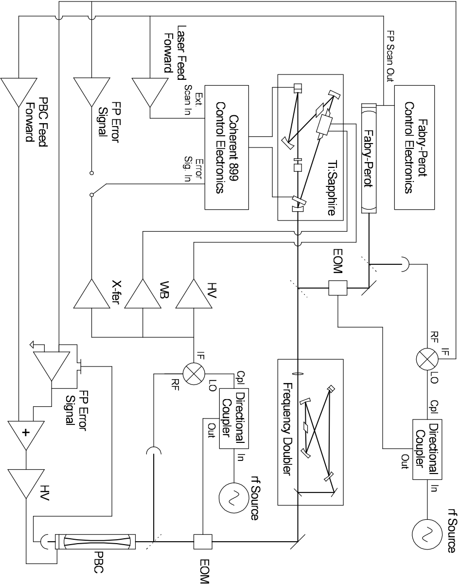
In order to increase the bandwidth of the frequency lock and narrow the line width of the laser to match that of the power-build-up cavity, an EOM was placed inside the laser cavity. The EOM used was a double-crystal assembly from LINOS Optics (PM 25 IR). The EOM was driven by a homemade electronics circuit.
The laser was locked to the power-build-up cavity using the fm-sideband technique Drever et al. 1983. The laser beam passed through an EOM (ConOptics 370) to which rf power of 4 W at 28 MHz was coupled via a resonant LC circuit. The laser beam was coupled on axis to the power-build-up cavity. The beam passed through a glass plate which picked off a small fraction of the light rejected from the input coupler of the cavity. This light was sent to an amplified fast photodiode (New Focus 1801, bandwidth 125 MHz). The signal from the photodiode was amplified and mixed down with the local oscillator to produce the error signal used to control the laser frequency.
In order to improve absolute frequency stability, the resonant frequency of the cavity was locked to a hermetically sealed, temperature-stabilized confocal Fabry-Perot interferometer at 816 nm (Burleigh CFT-500) with a free-spectral range of 150 MHz using a similar fm-sideband lock as that described above. The error signal from this locking system was sent to a high-voltage amplifier which controlled the piezo-ceramic-mounted mirror of the power-build-up cavity. Thus, the stable cavity provided the master frequency, with the power-build-up cavity serving as the secondary master for the laser. The frequency of the laser system was scanned over the profile of the atomic resonance by scanning the primary master Fabry-Perot cavity. Feed forward was sent to both the power-build-up cavity and the laser to help them track the frequency scans.
III.6 Fluorescence Detection
The number of atoms excited to the state was monitored by observing the fluorescence of the transition at 556 nm. A lucite light guide was used to send the fluorescent light to a photomultiplier tube (PMT, Burle 8850) outside of the vacuum chamber. A narrow-band interference filter, centered around 560 nm, with a pass band of 10 nm was placed on the front of the photomultiplier tube to reduce the scattered light reaching the PMT. The overall detection efficiency was such that of the atoms undergoing the 408-nm transition produced photoelectrons at the PMT photocathode. The photocathode was operated at V. The gain of the tube was measured to be at this voltage. The PMT current was fed into a Stanford Research Systems current preamplifier (SRS 570). The voltage output was recorded with a digital oscilloscope and saved to a computer.
III.7 Frequency Reference
Since the experiment relies on a detailed understanding of the spectral line shape of the transition over a region of MHz, a frequency reference with closely spaced frequency markers is needed. To this end, we have constructed a Fabry-Perot interferometer operating at 408 nm. The mirror spacing was chosen so that the transverse cavity modes overlap at frequency intervals of
| (29) |
with Budker et al. 2000. The interferometer mirrors each have a radius of curvature of , and are separated by 38.9 cm. This results in a spacing between the cavity resonances of 55.12 MHz.
IV Calculation of Line Shape
IV.1 Numerical Modeling
For a transition, there are generally four magnetic sublevels which must be included in a calculation. However, as discussed in Section II.2, the orientations of fields used in this experiment lead to excitation of a single energy eigenstate which is a superposition of the sublevels. Thus, we can neglect the structure of the upper state and treat the excitation of the atoms as a two-level problem.
The calculation was done using the density-matrix formalism. The Hamiltonian consists of the usual dipole coupling between the two states with an additional term along the diagonal which describes the energy shifts due to the ac-Stark effect
Here, is the dipole matrix element coupling the states, is the ac-Stark parameter, and is the oscillating electric field of the standing wave. We neglect the small residual running wave component of the field inside the cavity as it is times smaller than the standing wave component. The function is the amplitude of the oscillating electric field as a function of position. Since we are considering a two-level system, the tensor structure of the ac-Stark interaction is not included. In keeping with the discussion of Section II.2, the which appears here is given by
| (32) | ||||
The spatial variation of the electric field translates into a temporal variation as an atom passes through the laser beam. The electric-field amplitude inside the cavity is a standing wave with a fundamental-Gaussian profile
| (33) |
where is the electric-field radius of the Gaussian (following the convention of Ref. Siegman 1986), and is the wavelength of the light. The nominal direction of the atomic velocity is along . An atom with velocity
| (34) |
is subjected to an electric-field amplitude of
| (35) |
where we have chosen to be when the atom is in the middle of the laser beam. We have neglected since the change in as an atom crosses the laser beam is small. The largest angle an atom can have in the vertical direction and still intersect the laser beam is
| (36) |
where cm is the vertical dimension of the nozzle and cm is the distance between the nozzle and the interaction region. This means that the vertical position of the atom changes by only of the laser beam diameter as the atom crosses the beam.
A computer code was written in the programming language C to numerically solve the Louiville density-matrix equations (see for example Ref. Corney 1988, Ch. 15). The rotating-wave approximation was applied, and the equations were solved for the upper-state population using the semi-implicit Euler method Press et al. 1999. The program calculated the spectral line shape by integrating the density-matrix equations in time for atoms with a given transverse atomic-beam velocity , longitudinal atomic-beam velocity , initial position, and initial position. The program then integrated over each of these parameters with the proper distribution functions to arrive at the complete spectral line shape 11 1 For simplicity, we neglect correlations between longitudinal and transverse velocity distributions in the atomic beam. Estimated errors resulting from this approximations are included in the error budgets presented in Section V..
The upper-state population was integrated from a time to , where is the electric-field radius. The time integral was extended after to include an exponential decay with a decay time given by the lifetime of the state. The integration over the position, or vertical position of the atom relative to the laser beam, was performed from to . Calculations using these integration ranges were found to give consistent results with calculations with larger integration ranges.
The integration over the initial position was done by replacing the factor in the standing wave by a phase. Since the intensity of the standing wave repeats every , the integration in this phase was from to . Atoms traveling at large velocity see many periods of the standing wave as they traverse the laser beam. For this reason, the initial phase has little effect on the resulting signal. Thus for atoms with a magnitude of larger than a certain maximum value, the phase was set to 0 and the signal was not integrated over the phase. The magnitude of the maximum velocity was empirically chosen to be , where is the natural linewidth of the transition.
The integration over the longitudinal velocity assumed a distribution given for atoms escaping from a hole Ramsey 1990
| (37) |
where is the most probable velocity.
The transverse velocity distribution along used in the calculation was determined experimentally. The spectral line shape of the transition was recorded without the power-build-up cavity. This empirically determined line shape was then used as the input for the calculation.
A significant amount of effort was put into optimizing the program so that it was realistic to perform numerous calculations with different ac-Stark shift parameters and electric-field amplitudes. The time it took to perform a calculation varied depending on the values of and . For most of the calculations done in this work the time was min. for a single line shape consisting of 500 frequency points, running on a 3.6 GHz Pentium 4 processor.
IV.2 Calculated Line Shapes
Experimental data were taken at a variety of different light powers and dc-electric fields. The maximum electric field of the standing wave was varied between 1.5 and 7.5 kV/cm, and the dc electric field was varied between 5 and 15 kV/cm. Over this range of field values the line shape changes quite significantly.
Figure 4 shows the calculated line shapes for four different light powers (corresponding to the amplitudes of the light electric field shown in the figure), with a dc electric field of 5 kV/cm. The ac-Stark parameter assumed for these calculations is that estimated for the ground-state shift, . Figure 5 shows the line-shape variation with power for the same ac-Stark-shift parameter, but a dc electric field of 15 kV/cm. In both figures, the calculated signals have been divided by the square of the maximum electric field of the light.

While the details of the line shapes are quite complicated, the basic shape can be understood qualitatively by considering several different effects. The first effect we discuss is the saturation of the transition. Despite the smallness of the transition amplitude ( at ), the intense standing wave present at the highest light powers used in the experiment is sufficient to saturate the transition. This is clearly observed in the decrease of the power-normalized signal size as the power is increased. The effect is more pronounced for the calculations at a dc electric field of 15 kV/cm than for those at 5 kV/cm due to the increased Stark-induced amplitude at the higher electric field.

In addition to the overall decrease in the signal size, saturation also leads to hole-burning in the velocity distribution. The width of the dip is comparable to the homogeneous line width, which, in this case, is the power-broadened width.
While hole-burning changes the spectral line shape, it does not make the line shape asymmetric around zero detuning. To understand the asymmetry of the line shape we must include the effects of the ac-Stark shift. As can be seen from Figs. 4 and 5, the effect of the ac-Stark shift is not uniform over the profile of the line, suggesting a dependence on the atoms’ transverse velocity.
The source of the asymmetry can be understood in terms of an apparent frequency modulation resulting from the ac-Stark shifts. As the atoms travel through the laser beam the resonance frequency of the transition shifts depending on the intensity of the local light field. From an atom’s perspective this is equivalent to a frequency modulation of the laser light.
The depth of the frequency modulation (i.e., the maximum frequency shift) is determined by the magnitude of the ac-Stark shift and is given by
| (38) |
With the estimated ground-state shift and light powers used in the experiment, the depth of the modulation ranges between 0.28 and 7.4 MHz. The frequency of the modulation (as the atom moves between peaks and valleys of the standing light wave) is determined by the transverse velocity
| (39) |
where is the Doppler shift of an atom moving with transverse velocity . The factor of two in the above equation arises from the fact that the ac-Stark shift is quadratic so that the period of the shift is half that of the wave length of the light.
Since the apparent frequency of the modulation is determined by the transverse velocity [Eq. (39)], the effect is quite different for atoms with different . The transverse velocities where the character of the frequency modulation changes, depend on the size of the ac-Stark shift, and, as discussed below, on the homogeneous line width of the transition.
The character of frequency modulation is determined by the relative size of the depth of the modulation and the frequency of the modulation. In the case where , frequency modulation is characterized by the appearance in the spectrum of the light-frequency detuning as perceived by the moving atom of principal sidebands located at of the fundamental frequency. The sign of the amplitude of the sidebands is opposite for the high- and low-frequency sidebands. As the depth of the modulation is increased, the sidebands increase and higher-order sidebands develop. Eventually, the bulk of the amplitude shifts away from the fundamental frequency to the extreme frequencies. This evolution is shown in Fig. 6 for the electric-field amplitude and intensity of the light (proportional to the square of the amplitude).
An atom with a transverse velocity sees two “carrier” frequencies,
| (40) | ||||
| (41) |
corresponding to the Doppler shifts of the two counter-propagating waves which make up the standing wave. Since the resonant frequency of the transition is modulated, the detuning of the atomic resonance relative to the light frequency acquires sidebands. From the atom’s perspective, this appears as sidebands spaced a distance around and . Thus, the high-frequency side band of overlaps with and the low-frequency side band of overlaps with . However, since the high-frequency sideband for is positive, while the low-frequency sideband of is negative, there is a reduction of the amplitude at and an enhancement at . This leads to asymmetries in the resonant peaks at . As the transverse velocity is increased, the amplitude of the sidebands decreases and the height of the two Doppler-shifted resonances evens out.

Atoms with small transverse velocity pass through the laser beam without traversing multiple nodes and anti-nodes of the standing wave. The nature of the modulation is therefore not sinusoidal for these atoms, and cannot be parameterized in terms of . The atoms experiencing this regime have transverse velocities corresponding to Doppler shifts less than the transit line width which is kHz. Furthermore, if is less than the homogeneous line width (determined in this case by the power-broadened width), then the effects of the frequency modulation are smeared out. For these reasons, the regime of harmonic modulation where is much smaller than is never realized in the system under consideration.
Even if the atoms move exactly perpendicular to the light, there is spectral asymmetry due to the spatial dependence of the ac-Stark shift – the shift is different depending on the phase of the light wave the atoms see (determined by the y coordinate), and on the position of the atoms in the x-z plane.
V Analysis and Results
Line shapes of the type shown in Figs. 4 and 5 were generated over the appropriate range of transition amplitudes and a range of ac-Stark-shift parameters. The calculated line shapes were used to create an interpolating function in frequency, the ac-Stark-shift-parameter, and transition amplitude.
The calculations were related to the experimental spectral line shapes using the following parameterization of the calculations
| (42) |
where is the amplitude of the signal, and the function is the calculated line shape for a maximum electric field of the optical standing wave of , ac-Stark shift polarizability , Stark-transition polarizability , dc electric field , polarization angle , and frequency , centered around . The frequency term includes a multiplicative scaling factor . This parameter was introduced in order to account for any variation in the overall width of the data relative to the calculation. Such a variation might arise due to a misalignment of the atomic beam relative to the axis of the power-build-up cavity or a deviation of the velocity distribution from that measured without the cavity. We note that the parameters in Eq. (42) are not independent. Aside from scale and offset parameters, the calculated line shape depends only on the Rabi frequency of the transition () and the ac-Stark shift ().
Approximately twenty experimental scans were performed with a given dc-electric field, polarization angle, and light power. These scans were grouped together to form a set of data which was analyzed as described below. The dc-electric field was varied from 5 to 15 kV/cm between sets. Polarization angles of and relative to the dc-electric field were used. The light power was varied from to transmitted (corresponding to a maximum light electric field inside the cavity of 2 to 7.4 kV/cm). Data were taken at a total of 45 different field parameters.
The maximum light electric field inside the cavity, , was determined using the measured power transmitted through the cavity and the experimentally determined transmission coefficient of the cavity mirrors [Eq. (19)]. The dc-electric field was measured using the voltage divider mentioned in Section III.2. The value of the Stark transition polarizability was fixed in the analysis at [see Eq. (15)]. Effects arising from the uncertainty in , as well as an independent evaluation of from the present data are discussed below.
The power-normalized scans were individually fit to Eq. (42). Typical scans and fits for three different combinations of dc electric field and laser light power are shown in Fig. 7. For a given power and dc electric field the mean fit values of a set of scans were determined, and the distribution of the values was used to estimate the statistical error. The overall result, including sets at all of the dc-electric fields, polarization angles, and light powers used in the experiment is
| (43) |
where the error is determined from the statistical errors in each set of scans. The reduced chi squared for the data is 3.18 for 45 points. The large reduced chi squared is primarily due to inconsistency in the data taken at a dc electric field of 15 kV/cm with the data taken at lower fields. Table 1 shows the results for the different dc electric fields and Fig. 8 shows the dc-field dependence of the ac-Stark shift parameter.

| dc Electric Field | ac-Stark Shift | N | |
|---|---|---|---|
| 5 kV/cm | -0.3187(51) | 0.77 | 4 |
| 8 kV/cm | -0.3165(31) | 0.46 | 8 |
| 10 kV/cm | -0.3229(20) | 1.99 | 16 |
| Pol. | -0.3170(46) | - | 1 |
| Pol. | -0.3211(31) | 0.973 | 10 |
| Pol. | -0.3282(33) | 4.12 | 5 |
| 12 kV/cm | -0.3125(29) | 0.82 | 2 |
| 15 kV/cm | -0.3039(16) | 3.21 | 15 |

Excluding the data taken at 15 kV/cm gives a value of the ac-Stark shift of
| (44) |
with the reduced chi squared of 1.57 for 30 sets. Excluding everything but the 15 kV/cm data gives
| (45) |
with a reduced chi squared of 3.21 for 15 sets.
| Analysis Conditions | ac-Stark Shift | N | |
|---|---|---|---|
| -0.3123(11) | 3.18 | 45 | |
| Excluding 15 kV/cm data | -0.3188(14) | 1.57 | 30 |
| Only 15 kV/cm data | -0.3039(16) | 3.21 | 15 |
| -0.2953(11) | 7.53 | 45 | |
| Excluding 15 kV/cm data | -0.3112(14) | 1.88 | 30 |
| Only 15 kV/cm data | -0.2791(14) | 1.93 | 15 |
| -0.3290(11) | 2.46 | 45 | |
| Excluding 15 kV/cm data | -0.3292(14) | 1.92 | 30 |
| Only 15 kV/cm data | -0.3286(19) | 3.76 | 15 |
| Misaligned Velocity Distribution; | |||
| -0.3076(11) | 10.23 | 45 | |
| -0.2930(10) | 18.46 | 45 | |
| -0.3259(12) | 5.25 | 45 | |
| ‘s’ Parameter fixed at unity | -0.3384(10) | 9.16 | 27 |
| Atomic velocity | -0.2963(11) | 7.77 | 45 |
The discrepancy is also apparent in the parameter described above. The parameter has a clear dependence on the dc-electric field, going from at 5 kV/cm to at 15 kV/cm. A value of the parameter less than unity corresponds to an experimental line shape which is broader than the line shape calculated assuming .
This broadening of the line shape might suggest that the inconsistency in the data is a result of not properly accounting for saturation effects. However, there is no clear dependence of the extracted ac-Stark shift value on the light power, which one would expect if the saturation effects were the source of the discrepancy.
We analyzed the data in a number of different ways in order to understand this discrepancy as well as estimate systematic errors from calculational assumptions. The results of these investigations are tabulated in Tab. 2 and are discussed below.

The ac-Stark shift and the value of the Stark transition polarizability, , are highly correlated in the parametrization of the spectral line shape. The effects of the uncertainty in the value of were investigated by reanalyzing the data with the procedure described above assuming different values of . The results of this analysis are shown in Tab. 2. Figure 9 shows the dependence of the ac-Stark shift parameter on the dc electric field for the different values of the Stark transition polarizability. This analysis reveals a definite dependence of the ac-Stark shift parameter determined from the analysis on the value of . Furthermore, the discrepancy between the 15 kV/cm data and the lower field data was reduced when the data were analyzed with a value of the Stark transition polarizability of . However, the data are still inconsistent with reduced chi-squared of 2.46 for 45 points. This analysis suggests that the value of the Stark transition polarizability may be higher than the central value in Eq. (15), although consistent within the quoted uncertainty. Below, we describe a procedure for determining the value of the Stark transition polarizability from these data. This analysis provides a determination of the uncertainty in the ac-Stark shift parameter resulting from the uncertainty in . Based on the results presented in Tab. 2, we arrive at an uncertainty in the ac-Stark shift due to uncertainty in of .
Another possible source of experimental error arises from uncertainties in the atomic velocity distribution along the axis of the power build-up cavity. This uncertainty is the motivation for introducing the parameter described above and is highly correlated with it. The fact that the parameter is less than unity suggests that the center velocity of the atomic beam is not exactly perpendicular to the cavity axis. To analyze the effects of such a misalignment, the calculation described above was modified to include a Doppler distribution which was misaligned from the axis of the power-build-up cavity by . This misalignment corresponds to a Doppler shift of the two counter-propagating light waves constituting the standing wave by 2 MHz, respectively, as seen from the point of view of the atoms in the atomic beam moving with the most probable velocity. Misalignments larger than this lead to noticeable effects in the velocity distribution which were not present in the experimental data. We believe this to be an upper limit on the possible misalignment. The data were analyzed as before; the results are presented in Tab. 2. From these we determine that the uncertainty in the ac-Stark shift parameter due to the uncertainties in the alignment of the atomic beam with the cavity axis are . The values of the parameter resulting from this analysis ranged from 1.05 for E=5 kV/cm to 1.01 for E=15 kV/cm.
We also investigated the effect of including the parameter in the fit. We analyzed a fraction of the data (27 sets) fixing the parameter to unity. The fits using this procedure were not as good as the fits where was allowed to vary. In this case, the values of the ac-Stark shift parameter are largely determined by the wings of the Doppler distribution, since that is the only parameter available to broaden the line shape. The result of this analysis is shown in Tab. 2.
The longitudinal velocity distribution used in the calculation is also a possible source of uncertainty. We assume a standard longitudinal velocity distribution of effusive atoms escaping from a hole of [Eq. (37)], with the temperature fixed by the measured temperature at the rear (i.e., the coldest part) of the oven. However, atomic beams frequently deviate from this textbook distribution due to preferential scattering of the slow atoms (the so-called Esterman effect, see, for example, a discussion in Ref. Regan 2001). In addition, the oven is not at a uniform temperature; the temperature varies by over from front to back of the oven. This variation in temperature can modify the observed velocity distribution of the atomic beam. In order to investigate the effects of uncertainty in the longitudinal velocity distribution, data were analyzed using calculations assuming velocity distributions corresponding to different temperatures. The extracted values of the ac-Stark shift parameter are shown in Tab. 2. Assuming a maximal deviation in the central temperature of , we arrive at an uncertainty in the ac-Stark shift parameter of about .
Another key assumption in the calculation is that the problem can be reduced to that involving just two atomic levels. If the dc electric field and light field are the only fields present and are aligned appropriately, this is a correct assumption (see Sect. IV). However, if there are additional fields present, such as a magnetic field, this assumption may break down. With the experimental geometry used here (Fig. 2) the strong dc electric applied along splits the states from the state. A residual field along the - or -axes, would lead to mixing between the and states. However, since the Zeeman shifts () corresponding to the residual magnetic fields are small relative to the dc-Stark shifts, ( Bowers et al. 1999), this mixing is suppressed due to the strong dc electric field along the -axis and the two-level approximation still holds 22 2 Additionally, if this effect were to be the problem, one would expect larger internal inconsistencies in the data taken at low rather than at high dc electric field where the dc-Stark shifts are small. This is opposite to what we actually observed.. However, a residual magnetic field along the -axis would serve to split the degenerate states and the two-level treatment would be incorrect. To investigate this possibility, we utilized the magnetic-field coil normally used to compensate the ambient field in the -direction to apply a magnetic field parallel to the dc electric field. Data were then taken at different values of magnetic fields, which were analyzed as described above. The results are shown in Fig. 10. At large values of the magnetic field ( G), there is a dependence in the extracted value of the ac-Stark shift parameter as expected. However, no dependence was observed for data taken at magnetic field values that might realistically be present in the experiment. Thus, using the errors for the data taken with varying magnetic field we estimate the uncertainty in the ac-Stark shift parameter due to residual magnetic-field effects to be .

Misalignment of the optical field relative to the dc-electric field can also lead to a splitting of the energy eigenstates that are excited. With the geometry used in this experiment (Fig. 2), there are two possible kinds of such misalignment. One is an error in the angle between light field and dc electric field. Since the ac-Stark shift does not depend on the angle of the light field relative to the dc field in this geometry (see Sect. II.2), a misalignment of this kind does not lead to a breakdown of the two-level approximation, but changes the transition matrix element [Eq. (14)]. In the other kind of misalignment, the cavity axis has a component along the dc electric field. In this case, the assumption of a two-level system generally breaks down. However, for the case where the light field is polarized along the -axis, the dc electric field and the light field remain perpendicular. Thus, the above argument that was used to reduce the problem to that involving just two atomic levels is valid in this case, and the misalignment does not affect the extracted value of the ac-Stark-shift parameter. For a general polarization, a misalignment could influence the ac-Stark shift measurement. We can place a limit on the uncertainties arising from such possible misalignment by comparing the extracted ac-Stark-shift parameters for data taken with the angle of the light polarization relative to the dc electric field of with data taken at an angle of . Figure 11 shows the value of the ac-Stark shift parameter as a function of the polarization angle for data taken at a dc-electric field of 10 kV/cm. Using these results we are able to place a limit on the uncertainty in the ac-Stark-shift parameter due to misalignment of the light- polarization of .

Additional errors in the data arise from uncertainties in the dc-electric-field and light-field values. These errors, along with those discussed above are listed in Tab. 3. The uncertainty in polarization alignment was estimated based on the relative signal sizes at the different polarization angles. The uncertainty of is comparable to the measured degree of ellipticity in the transmitted light due to a birefringence of the cavity mirrors.
| Parameter | Uncertainty | Effect on |
|---|---|---|
| Transit Velocity | ||
| Calculational Approximations | n/a | |
| dc Electric Field | ||
| Polarization alignment | ||
| Residual Magnetic Field | ||
| Mirror Transmission | ||
| Power | ||
| Total Uncertainty | - |
Including all of the systematic errors listed in Tab. 3 we arrive at a systematic error of in the ac-Stark shift parameter, while the spread of the data is . We arrive at a final value of the ac-Stark transition polarizability of
| (46) |
In an attempt to determine the value of from the data, we also analyzed the results using a global fit of all data. In addition, the values of the Stark transition polarizability [Eq. (15)] and the frequency scaling parameter directly affect the extracted value of the ac-Stark polarizabilities. In order to properly account for this correlation, the variance of the data with the calculation was simultaneously minimized with respect to all three of these parameters. The data were analyzed by varying , , and and fitting the individual data scans to the amplitude, , and the center position . For a given set of , , and the of the individual fits were summed. This gave a global “ map,” using which a minimum was found with respect to , , and .
The value of the minimum of the global was normalized to unity. The errors were assigned by determining the deviations in , , and required to give a , where is the total number of data points used in all of the fits, and taking the appropriate projections along , , and . The results for the data grouped by field configurations as well as the result of a global fit to all of the data are shown in Tab. 4.
| dc Electric Field | ac-Stark Shift | s | N | |
|---|---|---|---|---|
| 5 kV/cm | -0.3261(38) | 2.301(18) | 0.9931(26) | 4 |
| 8 kV/cm | -0.3196(11) | 2.166(5) | 0.9724(8) | 8 |
| 10 kV/cm | ||||
| -0.3289(11) | 2.235(3) | 0.9788(21) | 1 | |
| -0.3327(9) | 2.283(8) | 0.9790(6) | 15 | |
| 12 kV/cm | -0.3248(13) | 2.233(4) | 0.9654(9) | 2 |
| 15 kV/cm | -0.3094(13) | 2.203(5) | 0.9622(5) | 15 |
| All Data | -0.3284(5) | 2.237(2) | 0.9730(3) | 45 |
There is good agreement between the results determined from the chi-squared map and the result determined from the fits to the individual data sets. Again, there is a discrepancy between the different electric-field sets. In addition, the extracted value of the Stark transition polarizability is inconsistent among the different electric field sets. Using the spread as an estimate of the uncertainty, we arrive at a measurement of the Stark transition polarizability of
| (47) |
which is in good agreement with and of comparable uncertainty as the previous measurement [Eq. (15)]. The error budget for the determination of is presented in Table 5. Considering the two measurements independent, we get the final value
| (48) |
| Parameter | Uncertainty | Effect on |
|---|---|---|
| Polarization alignment | ||
| Mirror Transmission | ||
| Power | ||
| Other | ||
| Total Uncertainty | - |
VI Conclusion
The results of the measurement of the ac-Stark shift of the transition at 408 nm [Eq. (46)] are in good agreement with estimates of the ac-Stark shift of the ground state [Eq. (18)]. The value of the ac-Stark shifts of this transition should not limit our ability to study parity nonconserving effects: the broadening due to ac-Stark shifts will not preclude resolving Zeeman components of the transition as necessitated by the current PNC-experiment scheme, and the present research has shown that lineshapes can be understood and modeled (see Fig. 7). In the future high-precision PNC experiments it will be necessary to work with a higher-finesse cavity. In that case, it may be possible to reduce the ac-Stark shifts by operating the cavity in the confocal regime, and expanding the laser beam to simultaneously excite a large number of the degenerate transverse modes.
An additional result of the present work is a new independent determination of the Stark transition polarizability . The result [Eq. 47] is consistent with the earlier result [Eq. 15] of Ref. Bowers et al. 1999 and has comparable uncertainty, but it does not rely on the knowledge of the decay branching ratios of the state.
VII Acknowledgements
The authors are grateful to David DeMille for initiating this research, and to Damon English, Derek Kimball, Chih-Hao Li, Angom Dilip, K. Tsigutkin, and Marcis Auzinsh for very useful discussions and criticism. This work has been supported by NSF, and by the Director, Office of Science, Office of Basic Energy Sciences, Nuclear Science Division, of the U.S. Department of Energy under contract DE-AC03-76SF00098.
References
- Wieman et al. (1987) C. E. Wieman, M. C. Noecker, B. P. Masterson, and J. Cooper, Physical Review Letters 58, 1738 (1987).
- Wood et al. (1999) C. S. Wood, S. C. Bennett, J. L. Roberts, D. Cho, and C. E. Wieman, Canadian Journal of Physics 77, 7 (1999).
- DeMille (1995) D. DeMille, Physical Review Letters 74, 4165 (1995).
- Bowers et al. (1999) C. J. Bowers, D. Budker, S. J. Freedman, G. Gwinner, J. E. Stalnaker, and D. DeMille, Physical Review A 59, 3513 (1999).
- Stalnaker et al. (2002) J. E. Stalnaker, D. Budker, D. P. DeMille, S. J. Freedman, and V. V. Yashchuk, Physical Review A 66, 31403 (2002).
- Budker and Stalnaker (2003) D. Budker and J. E. Stalnaker, Physical Review Letters 91, 263901/1 (2003).
- Happer (1970) W. Happer, Progress in Quantum Electronics 1, 47 (1970).
- Dupont-Roc and J. (1972) C. C.-T. Dupont-Roc and J., Physical Review A 5, 968 (1972).
- Cho et al. (1997) D. Cho, C. S. Wood, S. C. Bennett, J. L. Roberts, and C. E. Wieman, Physical Review A 55, 1007 (1997).
- Park et al. (2001) C. Y. Park, H. Noh, C. M. Lee, and D. Cho, Physical Review A 63, 032512/1 (2001).
- Park et al. (2002) C. Y. Park, K. Ji Young, S. Jong Min, and D. Cho, Physical Review A 65, 033410/1 (2002).
- Sobelman (1992) I. I. Sobelman, Atomic Spectra and Radiative Transitions, Springer Series on Atoms and Plasmas (Springer, New York, 1992), 2nd ed.
- Varshalovich et al. (1988) D. A. Varshalovich, A. N. Moskalev, and V. K. Khersonskii, Quantum theory of angular momentum: irreducible tensors, spherical harmonics, vector coupling coefficients, 3nj symbols (World Scientific, Singapore, 1988).
- Porsev et al. (1999) S. G. Porsev, G. Rakhlina Yu, and M. G. Kozlov, Physical Review A 60, 2781 (1999).
- Blagoev and Komarovskii (1994) K. B. Blagoev and V. A. Komarovskii, Atomic Data and Nuclear Data Tables 56, 1 (1994).
- Martin et al. (1978) W. C. Martin, R. Zalubas, and L. Hagan, Nat. Bur. Standards. 1978 pp. vii+411 (1978).
- Anderson et al. (1984) D. Z. Anderson, J. C. Frisch, and C. S. Masser, Applied Optics 23, 1238 (1984).
- Hood et al. (2001) C. J. Hood, H. J. Kimble, and J. Ye, Physical Review A 64, 033804/1 (2001).
- Drever et al. (1983) R. W. P. Drever, J. L. Hall, F. V. Kowalski, J. Hough, G. M. Ford, A. J. Munley, and H. Ward, Applied Physics B-Photophysics and Laser Chemistry B31, 97 (1983).
- Budker et al. (2000) D. Budker, S. M. Rochester, and V. V. Yashchuk, Review of Scientific Instruments 71, 2984 (2000).
- Siegman (1986) A. E. Siegman, Lasers (University Science Books, Sausalito, 1986).
- Corney (1988) A. Corney, Atomic and Laser Spectroscopy (Clarendon, Oxford, 1988).
- Press et al. (1999) W. H. Press, S. A. Teukolsky, W. T. Vetterling, and B. P. Flannery, Numerical Recipies in C: The Art of Scientific Computing (Cambridge University Press, New York, 1999), 2nd ed.
- Ramsey (1990) N. F. Ramsey, Molecular Beams (Oxford University Press, New York, 1990).
- Arfken and Weber (2005) G. B. Arfken and H.-J. Weber, Mathematical methods for physicists (Elsevier, Boston, 2005), 6th ed.
- Regan (2001) B. C. Regan, Ph.d. thesis, University of California (2001), available from the author or http://www.umi.com.
- Wood et al. (1997) C. S. Wood, S. C. Bennett, D. Cho, B. P. Masterson, J. L. Roberts, C. E. Tanner, and C. E. Wieman, Science 275, 1759 (1997).