Polyatomic Molecules Formed with a Rydberg Atom in an Ultracold Environment
Abstract
We investigate properties of ultralong-range polyatomic molecules formed with a Rb Rydberg atom and several ground-state atoms whose distance from the Rydberg atom is of the order of , where is the principle quantum number of the Rydberg electron. In particular, we put emphasis on the splitting of the energy levels, and elucidate the nature of the splitting via the construction of symmetry-adapted orbitals.
I Introduction
The recent advancement of ultracold physics has made possible the study of many interesting phenomena, ranging from the formation of molecules in a Bose-Einstein Condensate (BEC) Wynar et al. 2000; Gerton et al. 2000; McKenzie et al. 2002 to correlation effects in ultracold neutral plasmas Killian et al. 1999; Pohl et al. 2004, where in the former case the atoms are cooled to temperature in the nano-Kelvin range. Combined with narrow bandwidth lasers and high resolution spectroscopy Li et al. 2003, new phenomena can be studied involving high-lying Rydberg states which have a narrow spacing in energy of the order of 10 GHz. One such example is the theoretical prediction of the formation of ultralong-range dimers by a Rydberg atom and a nearby ground-state atom Greene et al. 2000, the so-called “trilobite” molecules. The potential well supporting the vibrational bound states is extremely weak compared to typical ground-state molecules. The depth of well is GHz for =30, where is the principle quantum number of the Rydberg atom, and scales as . The long-range nature of such system, bound at the equilibrium distance of the order of a.u., is rather unusual as well as the oscillatory feature at the bottom of the potential well. This class of ultralong-range dimers should be distinguished from another kind, due to the Rydberg-Rydberg interaction Boisseau et al. 2002, whose molecular resonance was observed in the experiments Farooqi et al. 2003; Marcassa et al. 2005.
In this paper we address the question if more than one ground-state atom can form, together with the Rydberg atom, a polyatomic molecule. We find, that shape and symmetry of such polyatomic molecules follow a systematics which is well understandable on the one hand side in terms of trilobite building blocks, that is, linear combinations of wavefunctions which describe the Rydberg atom and a single ground-state atom. From a more global perspective, these polyatomic molecules can be classified according to irreducible representations reflecting their symmetry properties, as it is well known in quantum chemistry.
So far, trilobites have not been identified experimentally. As the experimentally achieved density of ultracold atomic ensembles increases Sebby-Strabley et al. 2005, so does the likelyhood of detecting such molecular species. However, there are still open questions concerning the realizability of such a molecule under current experimental conditions. For example, the Rydberg electron is very likely to interact with multiple ground-state perturbers, and it is not so clear at first sight what the role of the Rydberg states is. Such scenarios will also concern the proposed “dipole blockade” scheme for quantum information processing Lukin et al. 2001. The characterization of polyatomic molecules involving one Rydberg and several ground-state atoms helps to understand the possible role of such ground-state perturber better.
Technically speaking, we extend the calculations done by Greene, Dickinson and Sadeghpour Greene et al. 2000 to include multiple ground-state atoms using the Fermi pseudo-potential treatment. More sophisticated methods exist Chibisov et al. 2002; Khuskivadze et al. 2002, but the results do not differ much, whilst the qualitative features are certainly captured which suffice for the purpose of the present article. Using the Fermi pseudo-potential also allows one to calculate easily a large system.
We investigate, in particular, the effect of placing the perturbers in a structured environment on the splitting of the adiabatic energy levels of the molecular system. We will use group theory to obtain the total wavefunction of the system in the framework of first-order perturbation theory via the construction of the symmetry-adapted orbitals. For the sake of clarity we restrict the investigation to atoms all lying in a plane (whereas the Rydberg electron of course lives in the physical 3D space). Atomic units are used unless stated otherwise.
II The Hamiltonian
First, we consider a ground-state atom with label located at distance from the Rydberg atom. The ground-state atom influences the electron by its polarization field, which has the form , where is the atomic polarizability. For Rb atoms, the experimentally determined value is Molof et al. 1974. To a good approximation, the potential – extremely short-ranged with respect to the extension of a Rydberg electronic wavefunction – can be mimiced by the Fermi pseudo-potential, namely Fermi 1934,
| (1) |
where is the s-wave energy-dependent scattering length of the Rydberg electron colliding with a neutral atom; its kinetic energy, and its distance from the mother ion. The s-wave phase shift can be calculated using the modified effective range theory by O’Malley et al O’Malley et al. 1961 and the zero-energy scattering length for triplet s-wave calculated by Bahrim et al Bahrim et al. 2001. The singlet scattering length is much smaller, and hence we do not expect it to influence the phenomena discussed here.
In the case of Rb atoms, the quantum defect is negligible for high -states (), which are quasi-denergate. They are therefore well represented by hydrogenic wavefunctions. The low- states, on the other hand, split away from the -manifold and do not interact with the high- states provided that the energy-dependent scattering length is sufficiently small. The high- states are also more interesting, because the Hilbert space is larger in this case, which produces a more flexible system, i.e. the different eigenstates are allowed to interfere with each other. This results in a highly-polarizable complex. In this paper, we consider only the high- class.
The total Hamiltonian of the Rydberg electron interacting with its mother ion and ground-state atoms can be written as
| (2) |
where the ionic Hamiltonian is
| (3) |
The potential is the -fold sum over the interaction Eq. (1) with all ground-state atoms, i.e.,
| (4) |
where labels the -th ground-state atom, and is the total number of ground-state atoms.
The effect of -wave electron scattering was neglected in our calculation, however, in the dimer case it was studied by Hamilton et al Hamilton et al. 2002 and Khuskivadze et al Khuskivadze et al. 2002.
III Determination of Adiabatic Energy Curves
Under the adiabatic approximation, the energy levels calculated from the Hamiltonian (including the perturbation) give, automatically, the electronic structure of the molecular system involving atoms. We determine a cut through the Born Oppenheimer (BO) potential surface for systems with , 3, and 4 ground state atoms which are uniformly placed on a circle with radius centered at the Rydberg core. These three cases correspond to linear, triangular, and square geometries, respectively. The cut we choose corresponds to the breathing mode, i.e. is varied. We calculate the BO curves using two methods: (i) the direct diagonalisation of ; and (ii) the projection operator method Levine 1975 to construct symmetry-adapted orbitals and determine the BO curves from standard perturbation theory. Both methods are accurate, but the latter gives a deeper insight into the quantum mechanical properties such as the energy degeneracy.
The Fermi pseudo-potential is usually valid for 25-30. For smaller principle quantum numbers, the scattering of and the polarization of the neutral perturber by the Rydberg atomic core are not independent of each other Fabrikant 1986. Here, we present calculations for , which also allows us to compare our results directly with that previously obtained for the Rb2 dimer Greene et al. 2000; Khuskivadze et al. 2002.
The eigenvalues from the unperturbed Hamiltonian, , yields simply the hydrogenic energy , so for convenience we set this to be zero throughout this article.
IV Collinear Triatomic Molecule (N=2)
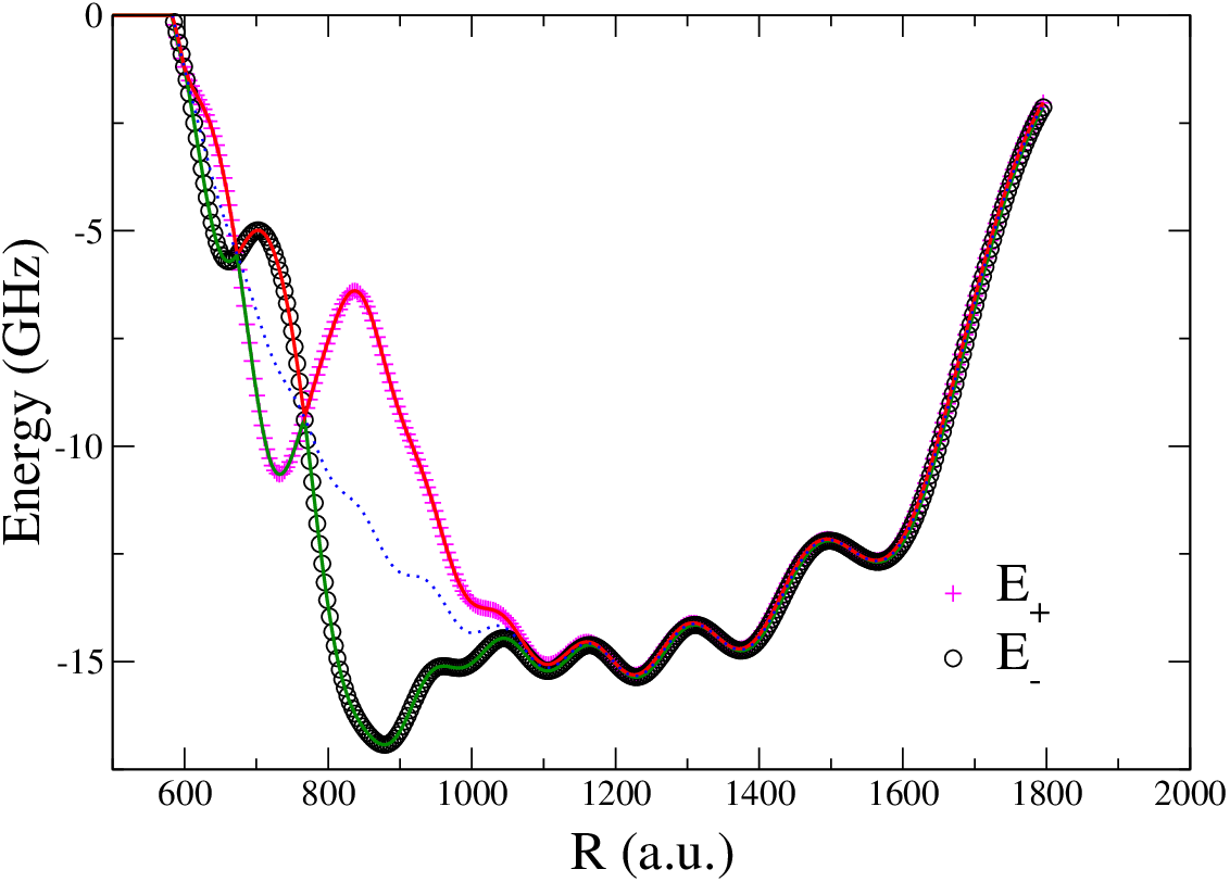
Consider two ground-state atoms (A and B) placed on either side of a Rydberg atom with distances forming a collinear triatomic molecule. This configuration corresponds to =2, and the numerical result of the BO curves are plotted in Fig. 1.
In order to understand the splitting of the energy levels, we use the perturbed state when only one of the two ground-state atoms is present as the building block for constructing the total electronic wavefunction. The perturbed state can be can be explicitly written as Omont 1977
| (5) |
where the index runs over all the degenerate states which includes all ’s and ’s with . We call this wavefunction the “trilobite” wavefunction since it produces the probability density like that drawn in Ref. Greene et al. 2000. The two wavefunctions, which clearly satisfy the parity of the collinear geometry, are
| (6) |
and
| (7) |
where the superscript A and B are the labels of the ground-state atoms; and are the trilobite wavefunctions when only atom A or B is present. By choosing the projection axis so that it aligns with the internuclear axis, the only degenerate states that contribute are those with non-zero value along . They are in this case the states with .
Using the above ansatz to calculate the expectation value yields immediately two energies and , which are distinguished by their parities:
where , and is the radial part of the hydrogenic wavefunction .

Hence, we see that, with the inclusion of the second perturber, two curves split away from the -manifold, with one corresponding to gerade and the other to ungerade symmetry. They both converge at large distance to the curve when only one ground-state atom is present. However, they split from each other approximately within (with ), which can be seen from the sum of the probability densities of even- and odd- states. They differ when the overlap is not exponentially small, see Fig. 2. This feature is general for all principle quantum numbers. The additional splitting also suggests that the system can be more stable with the inclusion of more than one neutral perturber, a situation we will investigate in more detail in Section V.
In Fig. 3, we show the contour plot of the probability density of the diatomic and triatomic systems at the interatomic distance , which corresponds to the deepest potential energy. The special minimum configuration can be most clearly identified by means of the classical Kepler orbits along which the two trilobite states of the molecule are scarred (see also Ref. Granger et al. 2001). Each Kepler ellipse has one ground-state atom in one of its foci and touches the other ground-state atom.


V Planar Polyatomic Molecules of Triangular and Quadratic Shape (N=3,4)
For , we choose to be perpendicular to the plane containing the atoms. Figure 4 illustrates the spacial geometry of the complexes. The degenerate states that contribute, i.e., the index in Eq. (5), are the states with being an even integer, exclusive of states. The results are shown in Fig. 5.

For the case, three energy eigenvalues split away from the -manifold, and as in the case of , beyond they converge to the BO curve for the dimer case. Note, however, that two of the energy levels are degenerate at any given distance within , indicating that there are additional symmetries preserved under the perturbation of the ground-state atoms. To elucidate these symmetries, we again use the trilobite state as basis functions to construct the relevant symmetry-adapted orbitals. But unlike in the previous collinear configuration, where taking account of the parity as the relevant symmetry is intuitive, we have to use a systematic approach for =3 or larger. A method which has been used extensively to find the symmetry-adapted orbitals is the projection operator method, which is expressed mathematically as Levine 1975
| (10) |
where is the operator for a particular symmetry operation , e.g., rotation or reflection, etc.. The and are, respectively, the dimension and the character of the -th irreducible representation (irrep) of the symmetry group, to which the system belongs, while is the order of the group. The sum extends over all symmetry operations in the group. This equation allows us to find the symmetry-adapted functions from any original basis set . The general proof of this proceedure can be found, for example, in section 6.6 of Ref. Schonland 1965.
The name of this procedure originates from the fact that the pre-factor in front of in the above equation can be viewed as a projection operator that projects the basis set into a basis set that diagonalizes the Hamiltonian matrix. In other words, and in Eq. (10) are vectors, and the operator
| (11) |
can be represented by a unitary matrix.
The configurations of =3 and 4 correspond to the symmetry groups and , and their character tables of the irreducible representations are shown in Table 1.
| E | |||
|---|---|---|---|
| 1 | 1 | 1 | |
| 1 | 1 | -1 | |
| 2 | -1 | 0 |
| E | |||||
|---|---|---|---|---|---|
| 1 | 1 | 1 | 1 | 1 | |
| 1 | 1 | 1 | -1 | -1 | |
| 1 | 1 | -1 | 1 | -1 | |
| 1 | 1 | -1 | -1 | 1 | |
| 2 | -2 | 0 | 0 | 0 |
We find that in the =3 case, the representation of the symmetry operations using the trilobite state as the basis set contains only two of the total three irreducible representations, and (see Table 1 and Appendix A.1 for details), which are one- and two-dimensional respectively. The symmetry-adapted orbitals constructed will then, according to the fundamental theory of quantum mechanics, consist of a non-degenerate and two degenerate states. They are, repectively, , and shown explicitly in Eq. (17), (18a) and (19) in Appendix A.1.
The energy expectation values,
| (12) |
calculated using the -functions are plotted in Fig. 5. As expected, the two curves belonging to overlap with each other at all distances . Note that applying onto any of the basis functions produces zero, which is a general feature when the irrep is not contained in the overall representation.
The same analysis for the symmetry reveals that the overall representation contains , , and (see Table. 1), with the first being one-dimensional, and the second and the third two-dimensional (see Appendix A.2 for detail). Hence, there are two sets of doubly-degenerate BO curves and a non-degenerate one. Applying Eq. (10), we obtain the symmetry-adapted orbitals , as shown in Eq. (23)-(26) in Appendix A.2. The adiabatic energy levels from the analytical and numerical results are plotted in Fig. 6. Again, the graph shows a perfect agreement between the two results.

VI Conclusion
We have used the Fermi pseudo-potential to model the effect neutral Rb ground-state atoms have on a Rydberg electron. Cuts through the resulting potential surface, adiabatic in the distance of the ground-state perturbers from the ionic core of the Rydberg electron, have been calculated for different arrangements of the ground-state atoms which form planar polyatomic molecules. We found that more ground-state atoms lead to more deeply bound molecules compared to the original diatom as studied by Greene and coworkers Greene et al. 2000. A systematic understanding of the structure and symmetry of such molecules can be gained by taking the trilobite (diatomic) wavefunction as a basic unit and constructing symmetry-adapted orbitals as demonstrated in Section IV and V. For two ground-state atoms the procedure is relative simple and intuitive, while three or more ground-state atoms require a systematic approach, such as the projection operator method.
In the case where is larger than the number of degenerate states , our method of constructing the perturbed wavefunction should still work, and will yield only linearly independent states.
The effect of -wave electron scattering plays an important role especially in hydrogen-like atoms. Our calculations can be extended into the case of higher partial wave scattering by using the appropriate pseudo-potentials formulated by Omont Omont 1977. Previous studies Hamilton et al. 2002; Khuskivadze et al. 2002 for dimers show that the potential curve of the -wave scattering crosses the potential well at , and could potentially destabilize the trilobite while also providing additional potential wells. It will be also interesting to see how the spatial arrangement of the atoms affect the energy of the system in this process, since the potential is now dependent on the gradient of the electronic wavefunction in the 3D space.
The present work is a first exploration of the possibility to form polyatomic molecules from a single Rydberg atom and a number of ground-state atoms. We have only determined a cut (at equal distances of the ground-state atoms to the Rydberg atom) through the multidimensional potential surface which resembles the potential for the breathing mode of the molecule. Future analysis and realistic assessment of the quantitative features of such species must include the vibrational motion of the atoms.
Appendix A Derivation of the Symmetry-adapted Orbitals
A.1 Planar Polyatomic Molecule with N=3
The molecule formed in this configuration has the symmetry of the point group . Using trilobite states as the basis set to contruct the corresponding representation, one obtains the following matrices,
| (13a) | ||||||
| (13b) | ||||||
| (13c) | ||||||
In the above notations, is the identity; denotes the rotation about -axis by angle ; and the ’s are the relfections through the planes perpendicular to the plane of the atoms, as indicated in Fig. 4.
It is clear that when one of the above operators, say , is applied on the original vector, the result is a rotation about in the counter-clockwise direction, assuming that is pointing perpendicularly into the paper, i.e.
| (14) |
From Eq. (13), the character of the representation in such basis set can be determined by taking the trace of each matrix, and they are summarized in the table below:
| E | |||
|---|---|---|---|
| 3 | 0 | 1 |
Here, we have used to denote the representation formed by the trilobite states. By inspecting the character table of the irreps of (Table 1), one immediately sees that the current representation is a direct sum of and , namely,
| (15) |
Now, we determine the projection operators in each irrep by using Eq. (11). The order of the group is , and the dimensions for and are and , respectively. Equation (11) then yields
| (16a) | ||||
| (16b) | ||||
| (16c) | ||||
Since contains only and , we need to apply only Eq. (16a) and (16c) to our basis set in order to obtain the symmetry-adapted orbitals. Acting the trivial operator on the trilobite wavefunction , we obtain the first symmetry-adapted orbital
| (17) |
The same equations are obtained if one acts on or which are obviously linearly-dependent. However, acting on , and gives, repectively,
| (18a) | ||||
| (18b) | ||||
| (18c) | ||||
A.2 Planar Polyatomic Molecule with N=4
Following the same procedure as in the case of , one finds the matrices of the symmetry operations in the point group in the present basis set as,
| (20a) | ||||||
| (20b) | ||||||
| (20c) | ||||||
| (20d) | ||||||
where the notations are as before, and the planes of reflections are indicated in Fig. 4.
The character of can again be determined by taking the trace of each matrix above, and they are:
| E | |||||
|---|---|---|---|---|---|
| 4 | 0 | 0 | 2 | 0 |
Again, from the character table of the irrep (Table 1), one finds that the representation is a direct sum of
| (21) |
Hence, we know that in this representation there are two one-dimensional and one two-dimensional irreps. Their corresponding projection operators can be obtained by applying Eq. (11), where in this case, , and , and are 1, 1 and 2, repectively. Therefore, the projection operators are
| (22a) | ||||
| (22b) | ||||
| (22c) | ||||
The symmetry-adapted orbitals can then be obtained in a similar way as in Appendix A.1, which yields the following four linearly-independent equations:
| (23) | ||||
| (24) | ||||
| (25) | ||||
| (26) |
References
- Wynar et al. (2000) R. Wynar, R. S. Freeland, C. R. D. J. Han, and D. J. Heinzen, Science 287, 1016 (2000).
- Gerton et al. (2000) J. M. Gerton, D. Strekalov, I. Prodan, and R. G. Hulet, Nature 408, 692 (2000).
- McKenzie et al. (2002) C. McKenzie, J. H. Denschlag, H. Häffner, A. Browaeys, L. E. E. de Araujo, F. K. Fatemi, K. M. Jones, J. E. Simsarian, D. Cho, A. Simoni, et al., Phys. Rev. Lett. 88, 120403 (2002).
- Killian et al. (1999) T. C. Killian, S. Kulin, S. D. Bergeson, L. A. Orozco, C. Orzel, and S. L. Rolston, Phys. Rev. Lett. 83, 4776 (1999).
- Pohl et al. (2004) T. Pohl, T. Pattard, and J. M. Rost, Phys. Rev. Lett. 92, 155003 (2004).
- Li et al. (2003) W. Li, I. Mourachko, M. W. Noel, and T. F. Gallagher, Phys. Rev. A 67, 052502 (2003).
- Greene et al. (2000) C. H. Greene, A. S. Dickinson, and H. R. Sadeghpour, Phys. Rev. Lett. 85, 2458 (2000).
- Boisseau et al. (2002) C. Boisseau, I. Simbotin, and R. Côté, Phys. Rev. Lett. 88, 133004 (2002).
- Farooqi et al. (2003) S. M. Farooqi, D. Tong, S. Krishnan, J. Stanojevic, Y. P. Zhang, J. R. Ensher, A. S. Estrin, C. Boisseau, R. Côté, E. E. Eyler, et al., Phys. Rev. Lett. 91, 183002 (2003).
- Marcassa et al. (2005) L. G. Marcassa, A. L. de Oliveira, M. Weidemüller, and V. S. Bagnato, Phys. Rev. A 71, 054701 (2005).
- Sebby-Strabley et al. (2005) J. Sebby-Strabley, R. T. R. Newell, J. O. Day, E. Brekke, and T. G. Walker, Phys. Rev. A 71, 021401(R) (2005).
- Lukin et al. (2001) M. D. Lukin, M. Fleischhauer, R. Côté, L. Duan, D. Jaksch, J. I. Cirac, and P. Zoller, Phys. Rev. Lett. 87, 037901 (2001).
- Chibisov et al. (2002) M. I. Chibisov, A. A. Khuskivadze, and I. I. Fabrikant, J. Phys. B: At. Mol. Opt. Phys. 35, L193 (2002).
- Khuskivadze et al. (2002) A. A. Khuskivadze, M. I. Chibisov, and I. I. Fabrikant, Phys. Rev. A 66, 042709 (2002).
- Molof et al. (1974) R. W. Molof, H. L. Schwartz, T. M. Miller, and B. Bederson, Phys. Rev. A 10, 1131 (1974).
- Fermi (1934) E. Fermi, Nuovo Cimento 11, 157 (1934).
- O’Malley et al. (1961) T. F. O’Malley, L. Spruch, and L. Rosenberg, J. Math. Phys. 2, 491 (1961).
- Bahrim et al. (2001) C. Bahrim, U. Thumm, and I. I. Fabrikant, J. Phys. B: At. Mol. Opt. Phys. 34, L195 (2001).
- Hamilton et al. (2002) E. L. Hamilton, C. H. Greene, and H. R. Sadeghpour, J. Phys. B: At. Mol. Opt. Phys. 35, L199 (2002).
- Levine (1975) I. N. Levine, Molecular Spectroscopy (John Wiley and Sons, Inc., 1975).
- Fabrikant (1986) I. I. Fabrikant, J. Phys. B: At. Mol. Opt. Phys. 19, 1527 (1986).
- Omont (1977) A. Omont, J. de Physique 38, 1343 (1977).
- Granger et al. (2001) B. R. Granger, E. L. Hamilton, and C. H. Greene, Phys. Rev. A 64, 042508 (2001).
- Schonland (1965) D. S. Schonland, Molecular Symmetry (Van Nostrand, Princeton, New Jersey, 1965).
- Salthouse and Ware (1972) J. A. Salthouse and M. J. Ware, Point Group Character Tables (Cambridge University Press, 1972).