Computing stationary free-surface shapes in microfluidics
Abstract
A finite-element algorithm for computing free-surface flows driven by arbitrary body forces is presented. The algorithm is primarily designed for the microfluidic parameter range where (i) the Reynolds number is small and (ii) force-driven pressure and flow fields compete with the surface tension for the shape of a stationary free surface. The free surface shape is represented by the boundaries of finite elements that move according to the stress applied by the adjacent fluid. Additionally, the surface tends to minimize its free energy and by that adapts its curvature to balance the normal stress at the surface. The numerical approach consists of the iteration of two alternating steps: The solution of a fluidic problem in a prescribed domain with slip boundary conditions at the free surface and a consecutive update of the domain driven by the previously determined pressure and velocity fields. For a Stokes problem the first step is linear, whereas the second step involves the nonlinear free-surface boundary condition. This algorithm is justified both by physical and mathematical arguments. It is tested in two dimensions for two cases that can be solved analytically. The magnitude of the errors is discussed in dependence on the approximation order of the finite elements and on a step-width parameter of the algorithm. Moreover, the algorithm is shown to be robust in the sense that convergence is reached also from initial forms that strongly deviate from the final shape. The presented algorithm does not require a remeshing of the used grid at the boundary. This advantage is achieved by a built-in mechanism that causes a smooth change from the behavior of a free surface to that of a rubber band if the boundary mesh becomes irregular. As a side effect, the element sides building up the free surface in two dimensions all approach equal lengths. The presented variational derivation of the boundary condition corroborates the numerical finding that a second-order approximation of the velocity also necessitates a second-order approximation for the free surface discretization.
pacs
47.55.Ca, 47.61.Jd, 47.11.Fg, 47.10.A-, 47.15.G-I Introduction
In the past decade the development of so-called “labs-on-a-chip” FigPin00; StoStrAjd04 has led to an increased interest in microfluidics,PolHay01; SquQua05; Thiele03 i.e. in the field of hydrodynamics with characteristic length scales of less than a millimeter. These flows are characterized by small Reynolds numbers and consequently governed by the Stokes equations. In the case of prescribed fluid domains with no-slip boundary conditions standard numerical methods exist for computing their solutions.DevFisMun02; ZieTay00
Recently, various experimental techniquesRamMorGre98; GutRatKel04 have been developed to induce and control flows in fluids which sit on a substrate without being confined by lateral and covering walls.WixStrGau04; GutMulHab05 In the experiments the fluid is kept together by its surface tensions both at the substrate and at the fluid–air interface. The stationary form that is assumed by the fluid–air interface is not given a priori. It results from an interplay of the internal streaming pattern, the internal pressure distribution and the surface tension. On the other hand, the form of the interface acts back on the flow. This mutual interaction of form and flow renders free boundary value problems fascinating but difficult. The relative importance of viscous flow and pressure, each compared to the influence of the surface tension, can be quantified by two dimensionless numbers, the capillary number and a generalized Bond number, respectively.
In the present work we consider a small water droplet (around 50 nl or less). The droplet sits on a flat substrate and is mechanically agitated by a body force.SAW Inside the droplet this body force then causes stationary pressure and flow fields which can lead to a significant deformation for the free surface. Sufficiently strong body forces may lead to the motion of the entire droplet, but this situation will not be considered here. The values of all, the Reynolds number, the capillary number, and the Bond number are assumed to range from zero up to unity. This corresponds to experimentally relevant situations.SriStrSch05; WixStrGau04; GutMulHab05
Several numerical approaches for determining free surface shapes have been proposed in the past. The suitability of the approaches depends on the size of the system, typical velocities, and the material properties, as well as on the resulting deformation of the fluid domain. They can roughly be classified into two groups: Either a fixed grid and a function describing the position of the free surface is used, or the computational mesh is moved together with the fluid domain, yielding a sharp surface representation by elements’ boundaries.
An established method of the first kind is the continuum method proposed by Brackbill et. al.BraKotZem92 They circumvented the discretization of the normal-stress boundary condition by introducing a body force density that is concentrated near the free surface. This force density accounts for the effect of surface tension. We have tested this method, which is implemented in the commercially available fluid-dynamics program FLUENT using a volume-of-fluid discretization. For a macroscopic system this method worked fine. The method, however, fails if the system is scaled down to the microfluidic parameter regime. In a simple test example we found that approximation errors of the free-surface boundary condition contributed to the force balance in the Navier–Stokes equations and were amplified in an uncontrolled manner. This typically gave rise to a spurious velocity field. It even occurred when we started the iteration with the known solution. Problems with this method have also been reported by Renardy & RenardyRenRen02 and by Popinet & Zaleski.PopZal99 Lafaurie et. al.LafNarScaZalZan94 find the spurious velocities to be of the order surface-tension/viscosity which is the dominant velocity scale for microfluidic systems. Thus, the existing continuum method appears to be inappropriate for the microfluidic parameter regime.
Another approach of the first kind has recently been proposed by Smolianski.Smolianski05 He uses finite elements and a level-set description for the free surface and calculates curvatures by derivatives of the distance-function. He still encounters spurious velocity fields proportional to the ratio surface-tension/viscosity.
Methods of the second kind, representing the free surface by a sharp interface are expected to work better in the microfluidic parameter regime. Algorithms in this class are often referred to as “moving mesh” or “ALE” methods and generally require more involved techniques, keeping the computational mesh feasible and not too distorted.
A technique of the second kind that has successfully been employed for tension-dominated free-surface problems is the boundary-element method.Pozrikidis92; ZinRotDav97 The dimensionality of the equations is reduced to the dimensionality of the surface which provides the basis for an efficient implementation. Unfortunately, this reduction can only be performed for Stokes equations with conservative body forces, which can be absorbed into the pressure term. In the present investigation we allow for non-conservative body forces which are of particular experimental relevance.WixStrGau04; GutRatKel04
Pioneering works for the finite-element implementation of the full free-surface problem were published by Scriven and coworkers.SaiScr81; KisScr83 They used spines to parameterize the movements of the computational mesh in coating flow and implemented Newton’s method for a Galerkin approximation scheme. This work was later continued under the designation “total linearization method” by Cuvelier and coworkers.CuvSch90; CuvSegSte86 Their description requires a height function for the free-surface position, which makes it necessary to use well-adapted coordinate systems like polar cylindrical or spherical ones. It must be known in advance if a free surface will overhang.
In the present paper we extend the works of Scriven and Cuvelier to arbitrary surface geometries. In our description, the parameterization of the free surface is given directly by the finite-elements’ boundary parameterization. Thus, neither spines nor a height function are needed. To properly account for intrinsic curvatures of the free surface, all equations are formulated in a fully covariant form that allows for all differential-geometric properties of the surface. An excellent reference for this formulation are the works of ArisAris89 and ScrivenScriven60 where the fluidic flow inside a curved free surface is described.
Recently, algorithms have been published that describe fully time-dependent free-surface flows, even in three dimensions.Bansch98; CaiSchBaeRekRaoSac00; WalGasJimKelSum05 In these works the free surface is moved mainly due to the kinematic boundary condition, i.e. it is advected passively. Concerning convergence, there has been a controversy if the kinematic or rather the normal stress boundary condition should be used to move the free surface. This issue was resolved by Silliman and Scriven who state that for capillary numbers below unity, the normal stress iteration converges well while a kinematic iteration eventually fails.SaiScr81 In addition, when the kinematic boundary condition is used for updating the free surface, the balance of normal stress that carries the effects of surface tension is not strictly imposed. It is used when implementing the weak form of the Navier–Stokes equations: In this context an integration by parts yields an integral of the normal stress over the free surface, which is then replaced by the corresponding surface-integral of the tension forces. Similar techniques are commonly used for problems with outflow boundary conditions or for Poisson’s equation with Neumann boundary conditions. The correctness of the technique has been justified for the outflow problem by Renardy.Renardy97 However, it is not evident if it also works in the case where the surface-tension terms dominate the whole problem. The question remains open, in which sense the boundary condition is satisfied. Therefore, we found it necessary in our examples to visualize the terms involved in the free-surface boundary condition, thus proving that they are correctly balanced.
An important result of a variational description of the tension terms is an improvement of the Newton algorithm controlling possible mesh distortions at the free surface. Many algorithms implementing the weak form of the capillary boundary condition encounter intrinsic instabilities of the boundary mesh when significant changes of the free surface take place. For the program surface evolver Brakke92 this manifests itself in shrinking and growing surface facets. Similar effects have been observed by BrinkmannBrinkmann02 and Bänsch.Bansch98 Our formulation of the capillary free surface is such that the free surface smoothly changes to the behavior of a rubber band when the boundary mesh becomes distorted. This leads to an automatic regularization of the mesh without the need of explicit remeshing or smoothing.
In Section II the mathematical formulation of the problem is presented in terms of differential equations, together with the boundary conditions and the relevant parameter regime. In Sec. III we then re-establish the bulk equations and their boundary conditions by variational techniques. For the free-surface we introduce a differential-geometric notation that allows us to write the boundary condition in a weak form. Up to this point a continuous description is used. Section IV introduces the discretization of the problem by the computational mesh. The formulation of the tension forces as the concurrent minimization of the free-surface area of single finite elements is a necessary requirement for the mentioned automatic regularization mechanism. Sec. V provides a short summary of the whole algorithm. In Sec. VI we present examples that show the accuracy of the algorithm and two further examples for different values of the capillary and Bond numbers. Mathematical and algorithmic details are deferred into the Appendices A–D.
II Statement of the problem
Throughout the paper, we shall write all equations in tensor notation for arbitrary curvilinear coordinate systems. This will considerably simplify the differential geometric notation in the following sections. For the formulation of the full Navier–Stokes equations in curvilinear coordinates we refer to Aris.Aris89 A repeated index that occurs in co- and contravariant positions is summed over, indices that are preceded by a comma denote covariant derivatives, and is the metric tensor of the underlying coordinate system.
II.1 The basic equations
We study incompressible and stationary flows, that are characterized by a small Reynolds number . Here, is the density of the fluid, its viscosity, and and denote typical magnitudes of length and velocity. Under these conditions the pressure field and the velocity field with components satisfy the Stokes equations LanLif63
| (1) | |||
| (2) |
where is the fluidic stress tensor, an external body force causing non-trivial streaming and pressure patterns within a domain . It can be split into its conservative part which can be displayed as the gradient of a potential and its non-conservative part with vanishing divergence. The domain may be bounded by rigid walls and by free surfaces, as e.g. a droplet sitting on a substrate. Equations (1) and (2) then are subject to boundary conditions at different parts of the boundary : First, the flow has to meet the kinematic boundary condition, requiring that the normal projection of a stationary velocity field vanishes at the boundary, i.e.,
| (3) |
At immobile sticky walls we use the no-slip boundary condition, according to which the velocity vanishes also in the tangential directions of the boundary, implying
| (4) |
Here, denotes the th component of the tangential vector ( for a two-dimensional surface). The remaining boundary is a free surface that dynamically adjusts its position such that the stress balance holds,
| (5) |
with the surface tension and the curvature . Note that we have omitted the gradient of the surface tension and thus exclude Marangoni effects. This simplifies the following calculations but does not present a principal restriction of our description.
Equations (1)–(5) have been simplified by assuming that the fluid in domain is surrounded by a medium of much smaller viscosity, which is the case e.g. for a water–air interface at room temperature. Therefore, the surrounding’s viscous stress contribution does not show up in the balance Eq. (5). We further assume that the ambient pressure is homogeneous. Since the pressure is determined by the Stokes equations only up to a constant, we can split it into a part with vanishing average and use the ambient pressure as an offset parameter which enters only in the normal stress balance (5),
| (6) |
II.2 The parameter regime
By transforming both, the bulk equation (2) and the free boundary condition (5) into dimensionless form employing viscosity-scaling, one observes that the system may be characterized by two relevant ratios of forces, given by the dimensionless numbers
| (7) |
Here, and denote typical magnitudes of length, velocity and the conservative part of the force density, respectively. Bo is a generalization of the Bond number which is usually defined in terms of gravitational forces only. The capillary number Ca measures the viscous contribution to the surface deformation. In a system with static boundaries and vanishing Reynolds number we can express the velocity scale by the typical magnitude of the non-conservative part of the driving force, namely . This yields an alternative definition of the capillary number similar to that of the Bond number,
| (8) |
These two numbers reflect the very different effects of the conservative and the non-conservative parts of the driving. In this sense, Ca provides also a measure for the spatial changes of the velocity field. For small Ca the flow is slow and changes smoothly, whereas for large Ca it may exhibit drastic gradients.
We propose our numerical scheme for the parameter regime where both, Ca, and Bo are of order unity or less. Thus, pressure gradients and viscous forces can deform the free surface significantly. The surface tension is large enough, however, in order to keep the whole fluid domain together, a pinch-off cannot occur. The viscosity renders the velocity field smooth over the whole fluid domain and prevents the existence of boundary layers. Because we consider only stationary flows in stationary domains according to Eqs. (2) and (3), and because we have set the substrate’s velocity to zero in Eq. (4), we always obtain pinned contact-lines. A rolling or slipping droplet would raise additional challenges regarding the stress near the contact-line that are beyond the scope of this paper.
III Continuous description of the problem
In order to clarify the numerical treatment of the free-surface boundary condition we first explore the physical origins of the balanced forces. We will then express each of them by the first variation of a functional. For Newton’s method it will be necessary to calculate also the second variation.
III.1 Physical aspects of the free-surface boundary condition: first variations
The surface tension term in the boundary condition (5) arises from the fact that an extended interface between two different phases “costs” free energy.LanLif63 To find the optimal configuration the surface is continually probing positions in its vicinity in order to minimize its free energy. For the case of an applied conservative force the system is static (), and the free-surface boundary condition is equivalent to a minimization of a free energy expression. This calculation is performed in Appendix A.

Due to its thermodynamic origin, the surface tension term results from a first variation of a functional. This carries over also to the dynamic case () in which the boundary condition (5) must hold at any instant of time. The contribution of the free surface to the system’s free energy is given by the integral of the surface tension over , where denotes the infinitesimal surface area,
| (9) |
Any smooth surface in a -dimensional space may be parameterized by surface coordinates () which determine the coordinates of points in -dimensional space on the surface. Both, surface and space coordinates are illustrated in Fig. 1. In our numerical studies we restrict ourselves to . The general framework, however, remains valid also for . The surface coordinates are taken from the parameter set . With running through the whole free surface is covered,
| (10) | |||
| (11) |
Here, is the th base vector in space. Throughout the paper we will always use Greek symbols for surface indices and Latin ones for space indices. The connection between surface and space coordinates is conveniently described by the surface-derivatives of the parameterization functions (cf. Aris,Aris89 p. 215), i. e.,
| (12) |
Understood as a contravariant -dimensional space-vector, represent the components of the th tangent vector to the surface. At the same time, is a covariant surface-vector. We can now construct the components of the surface’s metric tensor as the scalar products of these tangent vectors, namely
| (13) |
The metric tensor , its determinant and its inverse are nonlinear functions of the tangential vector components , see in Appendix B. The normal vector the normalized cross-product of two tangent vectors,
| (14) |
and the curvature is given as the trace of the tensor of the second fundamental form of the surface,
| (15) | |||
| (16) |
Using the parameterization (10) of the free surface, we demonstrate in Appendix B that the change of the free energy contribution with respect to a variation of the surface vectors is given by
| (17) |
By an integration by parts this expression can be cast into a form containing the curvature term of the free-surface boundary condition (5), i.e.,
| (18) |
(see Appendix C also for the case of varying surface tension). In this way, the curvature term in Eq. (18) that contains second spatial derivatives is replaced by a product of two terms, each containing a first derivative in Eq. (17). Especially for numerical applications it is much more favorable to work only with first derivatives. This trick has been used in the literature in different contexts.ZinRotDav97; Brakke92; Dziuk91; DecSie00; Bansch98 Seen from a physical perspective, version (17) of the equation is the more natural one. Here, one directly deduces that forces pulling along the tangential direction attempt to minimize the facet area of a mesh’s boundary. On the basis of single finite elements this perspective will be used below for stabilizing the computational mesh.
The left-hand side of Eq. (5), , is the normal fluidic stress at the boundary. We now recapitulate how this term can be understood as the result of a variational principle. In a stationary system with rigid immobile boundaries there is a balance between the power output due to viscous dissipation and the power input due to external driving. The total power output of the fluid, which we will denote with
| (19) |
vanishes. Additionally, for a prescribed domain , the Stokes equations yield those velocity and pressure fields that render the local power extremal (see Finlayson,Finlayson72 p. 271). Vice versa, from the vanishing first variation of ,
| (20) | ||||
| (21) | ||||
| (22) | ||||
| (23) |
the Stokes equations follow by setting the bulk contributions to zero. The boundary integral in the last row of Eq. (23) provides the fluidic stress in the free-surface boundary condition.
At this point we see that the two terms in the stress balance Eq. (5) have different physical origins. The surface tension is of thermodynamic (or rather of “thermostatic”) nature while the fluidic stress stems from dynamic considerations. The first results from minimizing a free energy, while the second stems from minimizing a power. Formally, this is expressed by the different variations and in the expressions in Eq. (23) and in Eq. (18). Already for dimensionality reasons they cannot be equal, neither can the functionals and be directly combined into one single variational principle.
From an algorithmic point of view one has to make a choice here: to approximate the free-surface boundary condition using either the or the as test-functions. In our Galerkin implementation of the problem we will use the ansatz functions as test functions. Therefore, in order to acquire a consistent numerical algorithm we have to approximate both, velocity and the geometry parameterization with finite elements of the very same order. This is the first central statement of the present work.
It was stated by BänschBansch98 (p. 42, cf. also citations 49 and 50 therein) that a second-order approximation of the surface parameterization yields a “good discrete curvature”, whereas a first-order one does not. The same can be seen below in Fig. 3. We are now able to substantiate his numerical observation with the underlying physical mechanism. The argument is similar to that for the celebrated Ladyzhenskaya–Babuska–Brezzi requirement that velocity gradients have to be approximated by the same order as the pressure. From a physical perspective this is not astonishing, because both are components of the same stress tensor.
III.2 Splitting the problem into two numerical systems
For free boundaries a twofold problem must be solved: (i) The unknown fluid domain is to be determined and (ii) the Stokes Eqs. (1) and (2) are to be solved within , using the boundary conditions (3)–(5). The latter themselves depend on the shape of via the normal vector at the boundary. Both parts of this problem cannot be processed independently.
In principle, there exist two options to deal with this combined problem. A first one is to implement a single numerical system for both, the flow variables and together with the geometry variables . We will not follow this direction but rather consecutively solve two smaller systems, one for the flow variables, depending on the current domain , and a second one for the parameterization of the boundary. We have chosen this approach because the problem is linear in the flow variables and highly nonlinear in the geometry variables . The nonlinearity is due to the appearance of the inverse surface metric in Eq. (17). Thus, solving the Stokes equations in the fluidic system, how we will call it, will be a standard problem, while the nonlinear search for the correct boundary shape will be done in the geometry system. Both systems are solved consecutively:
- 1.
Choose an initial domain .
- 2.
Until convergence repeat the following steps:
- (a)
Solve the fluidic system within the domain .
- (b)
Solve the geometry system using fixed values for the pressure and velocity variables. This results in an updated domain .
- (a)
In three-dimensional space the equations (3)–(5) pose four boundary conditions. They are one too many for the linear fluidic system to be fully determined. One boundary condition is thus used for updating the parameterization of the free surface.CuvSch90 The main challenge is the proper assignment of specific boundary conditions to the two systems in order to make them solvable, uniquely determined, and robust. It is clear that the no-slip boundary condition (4) at sticky walls applies only to the fluidic system. The free-surface boundary condition yet needs further consideration.
Here, again, a physical argument helps to choose the proper boundary condition. It is either the stress by the fluid or its velocity that is moving the free surface. Accordingly, either the normal stress balance (5) or the kinematic boundary condition (3) can be used by the geometric system to update the surface (see the discussion by Saito & ScrivenSaiScr81 and our remarks in the introduction). We choose our approach according to the following principle: The fluidic system should be well defined as a stationary system even if the boundary is fixed and is not part of the problem. If then the kinematic boundary condition were not imposed on the stationary flow, the velocity field would pass through the free surface which is also stationary. This excludes surface-updates by the kinematic boundary condition.
Until the correct boundary shape has been found, it is, in principle, possible that the surrounding flow forces the free surface into an arbitrary direction. By its very nature, however, the tension force stays always normal on the free surface. Only normal forces can be compensated by a free surface. As a necessary condition the tangential projection of the normal stress has to vanish.ill-posed Whenever tangential components emerge during the run of an algorithm, the result will be a numerical artefact. In the proposed scheme with two separated systems it is the fluidic system which must ensure the tangential components of the free boundary condition, i.e.,
| (24) |
Here, the surface tension has been set constant along the surface. For the velocity variables this constitutes a perfect slip boundary condition, which is similar to a Neumann boundary condition. We thus find the fluidic system to be fully determined and physically well defined even for fixed boundaries by the conditions (3), (4) and (24).
III.3 Second variation with respect to the surface parameterization
In a first implementation we used a direct and explicit update algorithm moving the boundary into normal direction with a step-width that is determined by a parameter and the residual of Eq. (25). The discretization of this update can be found below in Eq. (55). Depending on the value of this method exhibited strong instabilities as demonstrated below in Fig. 2. Although advanced techniques for determining an apt value for seem to exist (cf. the program surface evolver by BrakkeBrakke92), we prefer a Newton–Raphson iterative method. This has the advantage of a faster convergence and a less strong dependence on . A minor disadvantage is that it requires an additional variation of the surface free energy for the assembly of the geometry system. Using the same calculus as in Appendix B we find the second variation of the free energy contribution of a one-dimensional free surface,
| (26) | ||||
| (27) |
For a two-dimensional surface the corresponding variation contains two additional terms that are not given here for brevity. The last integral in Eq. (27) turns out to cause numeric instabilities in Newton’s method. This is a rather surprising fact, because the calculation that led to Eq. (27) consists of two straightforward variations. If the last integral in Eq. (27) is omitted the algorithm becomes stable and accurate (cf. the tests in Sec. VI.2).
It is not only the free energy contribution that depends on the shape of the surface. Also, the flow velocity, and by this, the viscous stress and the pressure depend on the shape. The formulation of the Newton method requires also the change of the fluidic stress integral due to changes of the free boundary,
| (28) |
The first two integrals on the right-hand side contain the changes of the normal vector (14) and the infinitesimal surface area due to changes of the boundary’s shape. Both can be calculated along the lines of Appendix B. The third integral expresses the change of the fluidic stress at the boundary due to changes of its position. The shape changes are communicated to the flow and pressure fields via the boundary conditions (3) and (24) of the Stokes equations. Unfortunately, this very indirect response of the stress tensor on the changes of shape cannot be expressed exactly. We therefore have to assume that this term can expressed by derivatives of the stress tensor, i.e.,
| (29) |
This means that the fluidic and the geometry system decouple to the extent that the stress tensor in the vicinity of the boundary is not affected by small boundary changes. We note that this is not a consequence of splitting the problem into two separate systems, but a general problem that equally applies to the combined approach. Altogether, the right-hand side of Eq. (28) becomes approximately
| (30) |
IV Discretization of the problem
We implemented the above equations by means of a Galerkin approximation scheme which is known to work well for minimization problems. As variables we introduced the velocity components and in - and -direction, respectively, the pressure , and additional variables and for the coordinates of the boundary parameterization vector . The continuous fields are discretized using ansatz functions, weighted with the corresponding degrees-of-freedom (DoF),
| (31) | ||||
| (32) | ||||
| (33) |
where the sum runs over all DoFs. The fluid velocity components are approximated by the second-order finite elements (FEs) and the pressure variable by first-order FEs . For the position variables we have predominantly used second-order FEs, but for accuracy and other testing reasons we also tried first-order FEs. We denote the position FEs with . All FEs are of the Lagrange family,DevFisMun02 having ansatz functions that are at exactly one node of the mesh and at all others. The DoFs are then equal to the function values at the nodes. This property is most convenient for the position variables that coincide with the coordinates of the node .
IV.1 The fluidic system
The fluidic system is implemented in a standard way. Equation (2) is tested with the second-order FEs , while the continuity Eq. (1) is tested with the first-order FEs . We have implemented the following linear equation for the DoFs, which are collected to vectors with components respectively,
| (34) |
with the entry matrices and entry vectors given by
| (35) | ||||
| (36) | ||||
| (37) | ||||
| (38) | ||||
| (39) | ||||
| (40) | ||||
| (41) | ||||
| (42) |
All integrals are assembled in a loop over the elements and the sides of the mesh, using a fifth-order Gaussian quadrature rule. The fluidic system could likewise implement the stationary Navier–Stokes equations with a small Reynolds number; we have chosen the Stokes equation for simplicity reasons here.
The boundary conditions are imposed by a constraints technique for the matrix and for the right-hand side in Eq. (34). A constrained DoF is expressed by an inhomogeneity plus a weighted sum of other DoFs,
| (43) |
which represent the boundary condition in question. The DoF is then completely eliminated from the linear system (34). By such constraint equations we implemented weak formulations of the kinematic boundary condition (3), i. e.,
| (44) |
of the no-slip condition at the walls
| (45) |
and of the tangential projection of the free-surface boundary condition (24),
| (46) |
The constraint equations differ only in the values of . The inhomogeneity is zero in all three equations. Non-zero inhomogeneities would result, if also a surface-gradient term of the tension were taken into account in Eq. (24), or if the rigid walls performed a tangential movement.
For the boundary condition (46), which is equivalent to an ideal slip condition, it is known that an improper choice of the normal direction can cause spurious contributions to the velocity field (see Behr,Behr04 Walkley et. al.,WalGasJimKelSum04 and our remarks stated in the introduction). In the presence of conservative forces only we did not find such spurious flows in our results.
The fact that the formulation of the free boundary condition in terms of the DoF-constraints (46) cross-links all DoFs residing at boundary nodes, presents a serious problem. Each of the DoFs is in principle linked to all its neighbors on the boundary. This leads to a nearly filled system-matrix which is unfavorable regarding memory capacity and computing time. We found that an iterative method can overcome this problem. Instead of cross-linking a boundary DoF with all its neighbors, for some of them we take their old values, as is detailed in Appendix D. After some iterations the full boundary condition (46) is established. The drawback of this scheme is that the constraint equations have to be re-assembled after every solution step of the fluidic system.
IV.2 The geometry system
The geometry system employs a Newton method to perform the nonlinear search for the correct boundary position. This scheme corresponds to a minimization of the free energy , while taking the fluidic stress into account. The boundary update equation can be written in a discretized form as
| (47) | ||||
where runs over the DoFs for each geometry variable, and and are understood as functions of the arrays , etc. containing the DoFs. For the Newton–Raphson method the geometry system repeatedly has to solve the linear system of equations BroSemMus95
| (48) |
where is a step-size parameter. In all applications we have used values of between and .
The search for the correct boundary shape is strongly nonlinear in the position variables. In order to remove the main nonlinearities, which are caused by the surface metric expressions and , the nodes of the elements are moved to their corresponding coordinates after each step of the geometry system. Then, all integrals can be performed directly on the elements’ edges. Also the normal vector can be taken from the elements’ sides. In the previous section we used a convenient variational notation to express the change of the free energy contribution by changes of the boundary parameterization. Essentially the same equations are obtained by differentiating the discrete version of with respect to the DoFs which are the nodal degrees of freedom of the corresponding variables. The only difference is that the variation in the continuous formulation must be replaced by the vectorial test-function , and the variation by its tangential derivative .
IV.3 Controlling the tangential displacements of boundary nodes
For a given discretization we must not only find the correct boundary shape, but its discretization should also remain well-proportionate. Very long and very short element sides cause badly conditioned matrices and make the whole algorithm unstable. Several algorithms implementing the weak form of the free-surface boundary condition encounter these intrinsic instabilities of the boundary mesh. For the program surface evolver this manifests itself in shrinking and growing surface facets. It is therefore recommended to monitor the mesh quality and remove too small or split too large elements.Brakke92 Similar effects were reported by Brinkmann.Brinkmann02
In Sec. III.2 the assignment of the boundary conditions to the fluidic and the geometry systems was described. There, we found that the presence of incompatible forces may easily destroy a free surface which essentially attempts to minimize the lengths of the free-surface sides in each element . Because all fluidic stresses are constrained to have only normal components, we are free to use additional tangential force components for keeping the boundary mesh as regular as possible. This can be done during the assembly of the system matrices by weighting the surface tension by the element’s side length , divided by the average length of all element sides contributing to the free surface. Of course, this weighting factor becomes ineffective if all sides have equal length. Any length difference of adjacent sides causes an additional force that tries to equalize them. The tension forces for each element side are then equivalent to a first variation of the functional , which describes a rubber band with Hookean forces. Instead of from Eq. (17) we thus assemble on each element
| (49) |
The second variations of and are not proportional to each other,
| (50) |
In the implementation we therefore took only the first term on the right-hand side of Eq. (50). In this sense we did not strictly implement the behavior of a rubber band, but yet a stabilized version of the free-surface tension terms. After convergence all boundary sides of the mesh representing the free surface have equal lengths and the extra terms do not change the behavior of the free surface.
V Summary of the algorithm
Here, we provide a short overview of the complete algorithm. The required steps are as follows:
- 1.
Choose an initial mesh and initial ambient pressure .
- 2.
Until convergence repeat the following steps:
- (a)
Smooth the inner mesh if it is too distorted.
- (b)
Repeatedly solve the fluidic system for , and , until the slip boundary condition is established.
- (c)
Subtract the average from .
- (d)
Solve the geometry system for the new boundary. At the same time search for the value of that keeps the volume unchanged.
- (e)
Set the mesh boundary nodes to the parameterization values of the geometry system.
- (a)
The fluidic system is assembled according to Eqs. (34)–(42) with constraints that account for the proper boundary conditions. To give the full algorithm at this point, we summarize also the terms of the geometry system. The update Eq. (48) is written as
| (51) |
with entries that are assembled per element ,
| (52) | ||||
| (53) | ||||
| (54) |
The remaining entries can be obtained by permutations of and together with and . Again, constraints have been used to keep the contact-lines pinned.
VI Numerical experiments
We performed all our test cases for a two-dimensional fluid. The programs were written using the open-source C++ library libmesh libmesh which allows to change the elements’ geometry in a user’s routine and provides a powerful constraint method.
VI.1 The instability of a “direct explicit update” algorithm
In our first numerical example we do not use Newton’s method with the update-rule (51), but instead with the direct and explicit update
| (55) |
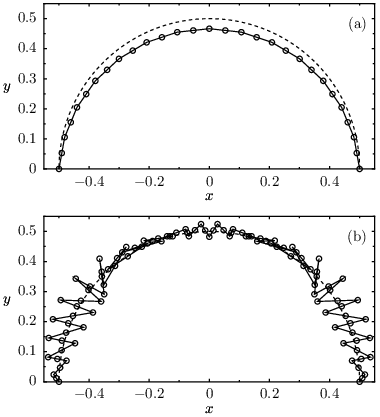
The stability of this update rule delicately depends on the step-size parameter . The allowed range of strongly depends on the size of the elements, the curvature, etc. Figure 2 depicts the most simple situation where a homogeneous pressure field deforms the boundary into a circular arc with radius . The update-rule (55) is stable for 14 FEs and a given step-size while it is unstable for the same step-size with 52 FEs.
VI.2 Testing the accuracy of the Newton algorithm
In order to confirm the accuracy of the curvature approximation we have tested two cases that can be solved analytically. Similar to the calculation in Appendix A, a prescribed pressure determines the free surface’s shape. Then, the approximation in Eq. (29) becomes exact and simplifies to
| (56) |
Thus, all possible approximation errors must be due to the discretization of the curvature.
Figure 3a depicts the most simple situation where a homogeneous pressure field deforms the boundary into a circular arc, as in the previous example. The free surface shape is approximated by the sides of 5 second-order FEs. In dimensionless units the surface tension is , and the prescribed pressure produces as the exact solution a circle with radius . The relative error of the numerically resulting radius, and thus also of the curvature, is about . This value has been obtained from the position of the topmost node. An alternative approach for calculating the approximation error is visualized in Fig. 3b. We calculated the normal vectors at each node from the resulting finite-element’s side. Due to the elements being second-order we got a single normal vector for second-order nodes. At vertices, where two elements meet and where the surface parameterization is not smooth, we averaged the two normal vectors. The curvature estimate at a node in Fig. 3b is then given by the curvature radius of a circle that connects the two neighbors of the specific node, given their appropriate normal vector. Thus, we explicitly reconstructed the curvature from the change of the normal vector along the surface. It is clear by construction that the normal vector of the contact-nodes cannot be correctly estimated. This causes the four outliers in Fig. 3b. All other nodes fit well.
A comparison with Fig. 2a, where the result of a first-order approximation can be seen, makes clear that it is crucial to use a second-order parameterization. The relative error of the curvature in Fig. 2a is , three magnitudes larger than in Fig. 3a.


In the next accuracy test, depicted in Fig. 4, the pressure is still prescribed, but it varies in space. As above, we apply a pressure for which the resulting boundary shape is known. Figure 4a illustrates the approximation of a sinusoidal boundary height function that is caused by the corresponding pressure field
| (57) |
Again, the approximation in Eq. (29) becomes exact, and we expect the same discretization errors as in the previous example. The curvature’s relative error is larger than in the previous example because the curvature is bigger compared to the number of nodes. Nevertheless, the error is still small enough to return the expected boundary shape within reasonable accuracy. It decreases with the number of approximating elements. If a first-order approximation is used it is much larger, maybe intolerably large.
Concerning the discretization errors of the curvature the accuracy test in Fig. 4 covers already the general case. According to the construction of the algorithm the flow exerts stress on the boundary only in normal direction. It makes no difference whether this stress is of viscous nature or due to a pressure difference.
VI.3 A deformed micro-droplet


In order to explicitly show that the quality of the curvature discretization does not depend on the origin of the applied normal stress we like to return to the introductory motivation for the present work. The previous examples were analytically solvable. The form and internal streaming of micro-droplets, however, cannot be determined analytically.
In the experiment the internal flow is agitated by a surface-acoustic wave (SAW) due to the acoustic streaming effect.Nyborg65 Because the very details of the SAW’s impact are not known, we here model it by a body force that is active in the fluid only, as depicted in Fig. 5. The force is concentrated in a narrow channel starting at the left contact point where the SAW hits the fluid and continuing into the fluid. It essentially carries the fluid along this channel, from the entry point of the SAW into the droplet, giving rise also to a back-flow.WixGut Additionally, the force has a strong conservative portion that is balanced by the pressure in the fluid.
The resulting stationary droplet shape and the internal velocity and pressure fields are presented in Fig. 6. The initial shape was a half-circle with the same two-dimensional volume. The deformed boundary consists of two regions, one with negative curvature (as the initial half circle) and another one at the right flank of the droplet with positive curvature. The material properties are those of water and air at room temperature, i. e. kg/ms and N/m. The – admittedly strange – deformation of the droplet qualitatively agrees with the experimentally observed jumping droplet in Fig. 4 of the publication by Wixforth et. al..WixStrGau04 The deformation is due to the large conservative contribution of the driving force and the resulting pressure. The viscous forces for the given velocities are far too weak to lead to a substantial deformation of the free surface. The capillary number for the illustrated flow is , the Bond number is around one. Although the free surface is significantly deformed, its discretization by finite-element sides is as regular as possible. Their lengths vary only by . This guarantees that the behavior of the boundary is indeed that of a free surface and is not disturbed by the automatic regularization technique described in Sec. IV.3. Figure 6d quantifies the normal stress condition. For each node we integrated the normal and the tangential component of the normal stress, weighted with the corresponding ansatz function of the node. The tangential component vanishes perfectly. The normal component coincides well with the reconstruction estimate of the curvature as in the previous examples. Thus, the free-surface boundary condition is indeed satisfied.
In order to prove that our algorithm can likewise produce stable results in the parameter regime we consider a droplet that is deformed only by viscous stress at the boundary. In Fig. 7 we have used the same non-conservative force that is visualized in Fig. 5, but we omitted the conservative part. Thus, the pressure was constant and . With the same water–air interface tension as in the previous example the droplet would hardly be deformed. To obtain a comparable deformation as in the previous case together with we took an artificial times smaller surface tension. In this example the stress that deforms the free surface depends much stronger on the shape of the surface itself. Thus, the approximation in Eq. (29) becomes questionable. It was necessary to reduce the step-size parameter to a smaller value than in the previous examples.
VII Summary and Outlook
Within this work we presented a weak formulation of free-surface boundary problems in arbitrary coordinate systems. The steps of the derivation are physically and mathematically founded using variational techniques for the Stokes equations and the differential geometry of the surface. We found that the applicability of different numerical treatments for the curvature terms depend strongly on the scales of the system. Our method is designed for Bond and capillary numbers assuming values from zero up to unity. Which one is larger plays no role.
A decisive benefit of our method is the automatic control of mesh regularity at a free surface. Many algorithms implementing the weak form of the free-surface boundary condition encounter intrinsic instabilities of the boundary mesh. Often, it is therefore necessary to create a completely new mesh after several iteration steps. Our formulation includes a smooth transition to the behavior of a rubber band when the boundary mesh becomes distorted. This leads to an inherent regularization of the mesh without affecting the behavior of the free surface.
As another important result we find that for physical reasons the geometry variables for the parameterization of the free surface should be approximated on the same level of accuracy as the velocity variables. This substantiates numerical observations reported by Bänsch.Bansch98
The quality of our numerical approach is tested by two analytically solvable examples. We explicitly plot the curvature of the free surface and the stress that causes the deformation. This confirms that the free surface boundary condition is indeed satisfied, not only in the weak sense which is implemented but even leads to a reliable reconstruction of the curvature by the normal vectors of the finite element’s sides. Two further examples illustrate that the ratio of capillary number and Bond number has only a weak influence on the stability of the algorithm.
The presented covariant formulation opens the possibility to utilize the powerful differential geometric description of free surfaces in finite-element implementations of the Stokes equations. It thus provides a natural approach to treat surfaces and interfaces with a richer behavior such as lipid vesicles containing bending stiffness, area constraints, and much more. Many potential applications can be found in the literature on lipid vesicle geometry, where more complicated expressions for the surface’s free energy contribution are in use.Guven04; CapGuvSan03; Seifert97
Extensions of the presented approach towards moving contact-lines, towards time-dependent flows and a three-dimensional implementation are possible. There are still some hurdles to be overcome that can be clearly seen in our derivation. One of them is the principally unknown mutual dependence of the stress tensor and the surface parameterization where we had to introduce the approximation (29). Another one is the understanding of the numeric instabilities caused by the last integral in second variation of the surface’s free energy (see Eq. (27)).
These extensions would also provide a solid basis for the theoretical understanding of particle transport in surface-acoustic-wave-driven flows.SriStrSch05; StrSchBei04; StrFroGut; KosSchTalHae05
Acknowledgements.
We gratefully acknowledge our experimental partners in the group of Prof. Achim Wixforth, Univ. Augsburg, and the developers of the libmesh project. This work was supported by the Deutsche Forschungsgemeinschaft (DFG) via grant 1517/25-1, SFB 486 and the Graduiertenkolleg: Nichtlineare Probleme in Analysis, Geometrie und Physik.Appendix A A static droplet in Cartesian coordinates
The aim of this appendix is to recall the variational techniques in a simple three-dimensional Cartesian setup before going to arbitrary coordinates in appendix B. The argumentation is similar to the one given by Cuvelier.CuvSch90
We describe the special case where the fluid’s two-dimensional free surface can be described by a height function
| (58) |
which is non-zero over a certain region . The Stokes equations for the static situation with a conservative force reduce to
| (59) |
with the solution . The undetermined homogeneous term will be identified as the Lagrange multiplier for the constraint of constant volume .
The free energy of the system consists of the surface-integral of the constant surface tension and the volume-integral of the potential
| (60) |
with
| (61) |
The Euler-Lagrange equation for finding the extremal by varying is then
| (62) | ||||
| (63) |
where is the curvature of , given by
| (64) |
Because the pressure is given by the potential, the Euler-Lagrange equation is equivalent to the free-surface boundary condition for a static fluid,
| (65) |
At this point it is easy to see that plays the role of a Lagrange multiplier for a volume constraint. Adding the term
| (66) |
to gives an additional constant in the Euler-Lagrange equation, just as the pressure offset . Because is yet undetermined we may identify it with .
Appendix B Variational calculus for the surface’s parameterization
In order to prove equality (17) we express the change of the surface’s free energy functional (9) by the change of the Jacobi determinant of the surface parameterization. With the infinitesimal surface area the variation of the surface free energy becomes
| (67) |
The dependence of on the tangent vectors follows from its definition as the determinant of the surface metric. For a two-dimensional surface it reads
| (68) |
where is the permutation symbol in two dimensions,
| (69) |
which is a relative surface tensor with weight . The absolute tensor results as
| (70) |
This is analogous to the completely antisymmetric tensor in three dimensions, described in detail by Aris.Aris89 With the antisymmetric tensor we obtain the inverse surface metric as
| (71) |
A formal derivative of (68) yields
| (72) | ||||
| (73) |
which can be inserted into (67) to give the desired result (17).
For a one-dimensional curve in two-dimensional space the same formula can be derived, but the notation may be somewhat confusing. Summation over the single surface index makes no sense, nevertheless, we still have to distinguish between co- and contravariant relative tensors, i. e.,
| (74) | |||
| (75) |
The formal derivative then becomes
| (76) |
which completes the result for the one-dimensional surface.
Appendix C Integration by parts of the tension forces
In order to see that Eq. (18) follows from Eq. (17) we remove the surface covariant derivative from by an integration by parts and obtain
| (77) |
where the covariant surface vector is tangential to and normal to . We can express the surface-derivatives by the tensor of the second fundamental form of the surface from Eq. (16) (cf. to Aris,Aris89 p. 216),
| (78) |
arriving at
| (79) |
We have used the definition of the curvature as the trace of the tensor of the second fundamental form as in Eq. (15). For a two-dimensional surface this is twice the mean curvature , for a one-dimensional surface we have only one entry .
As consistent with the standard literature,LanLif63; Aris89 the term from Eq. (17) comprises a curvature term in normal direction
| (80) |
and a term accounting for the surface-gradient of . The space vector
| (81) |
is tangential to the surface. The third term on the right-hand side of Eq. (77), which is an integral over the contact-line , vanishes because for a pinned droplet vanishes on the contact-line.
Appendix D Invoking constraints for the slip boundary condition

The tangential components of the free-surface boundary condition correspond to a slip boundary condition. When this condition is expressed as a set of constraints for the DoFs, we obtain one equation like (46) per each DoF at the free surface. Because the derivatives of the ansatz functions from (31) generally do not vanish at proximate nodes, the constraint equations contain non-vanishing weights for all DoFs that are located on the same element. Therefore, the constraints for DoFs that are connected to two adjacent elements create inter-dependencies of DoFs also on other elements. This is illustrated in Fig. 8a. As a result, all DoFs on the free surface implicitly depend on each other. After the constraints are re-sorted such that DoFs are constrained only in terms of non-constrained ones, it turns out that the free-surface DoFs depend on all DoFs in the element layer near the surface.
As a strategy to avoid this full dependency we replace the constraint equation of type (43) by
| (82) |
where the sums run over two complementary sets and . The DoFs in contribute to the constraint for in the usual way, while those in have been substituted by their old values and thus contribute to the inhomogeneity. There is some freedom in the choice, which of the participating DoFs in one element are in and which are taken into . We found that the combination illustrated in Fig. 8b works well: For the DoFs located at element vertices we take the DoFs that belong to adjacent nodes on the free surface as inhomogeneities; all other constraining DoFs are located at inner nodes and are not constrained. The DoFs located at the second-order nodes on the free surface acquire their full constraints. When all constrained DoFs are expressed by non-constrained DoFs, then the resulting constraint equations will only contain DoFs that are located at inner nodes of three adjacent elements. This presents a sufficient decoupling of the constraint equations to yield an efficient algorithm.
Although the boundary condition given by Eq. (82) is not the correct one when the true velocity field has not yet been determined, it still improves as the velocity field tends to the proper solution. Thus, there is hope that the correct boundary condition is established by the successive use of Eq. (82) using increasingly good values for the values . In numerical experiments the scheme for splitting the cross-dependencies as illustrated in Fig. 8b turned out to be the only one that works. In the examples of Figs. 6 and 7, it took about 20 iteration steps to establish the correct boundary condition from scratch, and 5 iteration steps to re-establish it after a change of the mesh. This could be readily observed because after the first iteration step the velocity field exhibited oscillations at the boundary nodes that ceased during iteration.
References
- (1) D. Figeys and D. Pinto, “Lab-on-a-chip: A revolution in biological and medical sciences,” Anal. Chem. 72, 330A (2000)
- (2) H. A. Stone, A. D. Stroock, and A. Ajdari, “Engineering Flows in Small Devices: Microfluidics Toward a Lab-on-a-Chip,” Annu. Rev. Fluid Mech 36, 381 (2004)
- (3) N. A. Polson and M. A. Hayes, “Microfluidics controlling fluids in small places,” Anal. Chem. 73, 312A (2001)
- (4) T. M. Squires and S. R. Quake, “Microfluidics: Fluid physics at the nanoliter scale,” Rev. Mod. Phys. 77, 977 (2005)
- (5) U. Thiele, “Open questions and promising new fields in dewetting,” Eur. Phys. J. E 12, 409 (2003)
- (6) M. O. Deville, P. F. Fischer, and E. H. Mund, High-Order Methods for Incompressible Fluid Flow (Cambridge University Press, Cambridge, 2002)
- (7) O. C. Zienkiewicz and R. L. Taylor, The finite element method. Volume 3: Fluid Dynamics (Butterworth-Heinemann, Oxford 2000)
- (8) A. Ramos, H. Morgan, N. G. Green, and A. Castellanos, “AC electrokinetics: a review of forces in microelectrode structures,” J. Phys. D: Appl. Phys. 31, 2338 (1998)
- (9) Z. Guttenberg, A. Rathgeber, S. Keller, J. O. Rädler, A. Wixforth, M. Kostur, M. Schindler, and P. Talkner, “Flow profiling of a surface-acoustic-wave nanopump,” Phys. Rev. E 70, 056311 (2004)
- (10) A. Wixforth, Ch. Strobl, Ch. Gauer, A. Toegl, J. Scriba, and Z. Guttenberg, “Acoustic manipulation of small droplets,” Anal. Bioanal. Chem. 379, 982 (2004)
- (11) Z. Guttenberg, H. Müller, H. Habermüller, A. Geisbauer, J. Pipper, J. Felbel, M. Kielpinski, J. Scriba, and A. Wixforth, “Planar chip device for PCR and hybridization with surface acoustic wave pump,” Lab on a Chip 5, 308 (2005)
- (12) In an experimental realization the body force may be caused by a surface-acoustic wave (SAW) that travels over the substrate’s surface and rushes into the droplet.WixStrGau04 The fast motion of the SAW is damped by the fluid, giving rise to a body force via the acoustic streaming effect.Nyborg65
- (13) K. Sritharan, C. J. Strobl, M. F. Schneider, Z. Guttenberg, and A. Wixforth, “Acoustic mixing at low Reynolds numbers,” (submitted)
- (14) J. U. Brackbill, D. B. Kothe, and C. Zemach, “A Continuum Method for Modeling Surface Tension,” J. Comput. Physics 100, 335 (1992)
- (15) Y. Renardy and M. Renardy, “PROST: A parabolic reconstruction of surface tension for the volume-of-fluid method,” J. Comput. Phys. 183, 400 (2002)
- (16) S. Popinet and S. Zaleski, “A front-tracking algorithm for accurate representation of surface tension,” Int. J. Numer. Meth. Fluids 30, 775 (1999)
- (17) B. Lafaurie, C. Nardone, R. Scardovelli, S. Zaleski, and G. Zanetti, “Modelling merging and fragmentation in multiphase flows with SURFER,” J. Comput. Phys. 113, 134 (1994)
- (18) A. Smolianski, “Finite-element/level-set/operator-splitting (FELSOS) approach for computing two-fluid unsteady flows with free moving interfaces,” Int. J. Num. Meth. Fluids 48, 231 (2005)
- (19) C. Pozrikidis, Boundary Integral and Singularity Methods for Linearized Viscous Flow (Cambridge University Press, Cambridge, 1992)
- (20) A. Z. Zinchenko, M. A. Rother, and R. H. Davis “A novel boundary-integral algorithm for viscous interaction of deformable drops,” Phys. Fluids 9, 1070 (1997)
- (21) H. Saito and L. E. Scriven, “Study of Coating Flow by the Finite Element Method,” J. Comput. Phys. 42, 53 (1981)
- (22) S. F. Kistler and L. E. Scriven, Coating Flows, in Computational analysis of polymer processing, edited by J. R. A. Pearson (Applied Science Publishers, Barking, Essex, 1983) Ch. 8
- (23) C. Cuvelier and R. M. S. Schulkes, “Some numerical methods for the computation of capillary free boundaries governed by the Navier-Stokes equations,” SIAM Review 32, 355 (1990)
- (24) C. Cuvelier, A. Segal, and A. A. van Steenhoven, Finite Element Methods and Navier-Stokes Equations (D. Reidel, Dordrecht, 1986)
- (25) R. Aris, Vectors, Tensors, and the Basic Equations of Fluid Mechanics (Dover Publications, New York, 1989)
- (26) L. E. Scriven, “Dynamics of a fluid interface. Equation of motion for Newtonian surface fluids,” Chem. Eng. Sci. 12, 98 (1960)
- (27) E. Bänsch, Numerical methods for the instationary Navier-Stokes equations with a free capillary surface (Habilitation thesis, Albert-Ludwigs-Universität Freiburg, Freiburg, 1998)
- (28) R. A. Cairncross, P. R. Schunk, T. A. Baer, R. R. Rekha, and P. A. Sackinger, “A finite element method for free surface flows of incompressible fluids in three dimensions. Part I. Boundary fitted mesh motion,” Int. J. Numer. Meth. Fluids 33, 375 (2000)
- (29) M. A. Walkley, P. H. Gaskell, P. K. Jimack, M. A. Kelmanson, and J. L. Summers, “Finite element simulation of three-dimensional free-surface flow problems,” J. Sci. Comput. 24, 147 2005
- (30) M. Renardy, “Imposing ‘no’ boundary condition at outflow: Why does it work?” Int. J. Num. Meth. Fluids 24, 413 (1997)
- (31) K. A. Brakke, “The Surface Evolver,” Experimental Mathematics 1, 141 (1992)
- (32) M. Brinkmann, Benetzung lateral strukturierter Oberflächen (PHD thesis, Universität Potsdam, Potsdam, 2002)
- (33) L. D. Landau and E. M. Lifshitz, Fluid mechanics (Pergamon Press, Oxford, 1963)
- (34) G. Dziuk, “An algorithm for evolutionary surfaces,” Numer. Math. 58, 603 (1991)
- (35) K. Deckelnick and K. G. Siebert, “-convergence of the discrete free boundary for obstacle problems,” IMA J. Numer. Anal. 20, 481 (2000)
- (36) B. A. Finlayson, The Method of Weighted Residuals and Variational Principles (Academic Press, New York, 1972)
- (37) As a simple demonstration we consider a problem that is similar to the well-known catenary setup. A curve, representing the one-dimensional surface, in two-dimensional-space is assumed to be fixed at its endpoints. A homogeneous force should act in the direction normal to the connecting line between the endpoints. If the curve is physically realized by a chain of rigid or elastic elements, its shape is given by a catenary or a parabola, respectively. But if the curve had to be realized by the free surface of a fluid, this problem is ill-posed and does not possess a stationary solution. The free surface then can only compensate normal forces and its shape would be a straight line. On the other hand, its curvature would then be zero and therefore could not compensate the external force. Hence, no solution exists.
- (38) M. Behr, “On the application of slip boundary condition on curved boundaries,” Int. J. Numer. Meth. Fluids 45, 43 (2004)
- (39) M. A. Walkley, P. H. Gaskell, P. K. Jimack, M. A. Kelmanson, and J. L. Summers, “On the calculation of normals in free-surface problems,” Commun. Numer. Meth. Engng. 20, 343 (2004)
- (40) I. N. Bronshtein and K. A. Semendyayew, Handbook of Mathematics (Harri Deutsch, Thun, Frankfurt a. M., 1985)
- (41) B. S. Kirk, J. W. Peterson, R. Stogner, and S. Petersen, libMesh – A C++ Finite Element Library, [available at http://libmesh.sourceforge.net]
- (42) W. M. Nyborg, “Acoustic Streaming,” Physical Acoustics 2B, 265 (1965)
- (43) A. Wixforth, Z. Guttenberg (private communication)
- (44) J. Guven, “Membrane geometry with auxiliary variables and quadratic constraints,” J. Phys. A: Math. Gen. 37, L313 (2004)
- (45) R. Capovilla, J. Guven, and J. A. Santiago, “Deformations of the geometry of lipid vesicles,” J. Phys. A: Math. Gen. 36, 6281 (2003)
- (46) U. Seifert, “Configurations of fluid membranes and vesicles,” Adv. Phys. 46, 13 (1997)
- (47) C. J. Strobl, C. Schäflein, U. Beierlein, J. Ebbecke, and A. Wixforth, “Carbon nanotube alignment by surface acoustic waves,” Appl. Phys. Lett. 85, 1427 (2004)
- (48) C. Strobl, T. Frommelt, Z. Guttenberg, and A. Wixforth, “Particle Separation in a SAW-driven microfluidic system with continuous flow,” (submitted),
- (49) M. Kostur, M. Schindler, P. Talkner, and P. Hänggi, “Chiral separation in microflows,” Phys. Rev. Lett. 96 014502 (2006)