Fits, and especially linear fits, with errors on both axes,
extra variance of the data points and other complications
Abstract
The aim of this paper, triggered by some discussions in the astrophysics community raised by astro-ph/0508529, is to introduce the issue of ‘fits’ from a probabilistic perspective (also known as Bayesian), with special attention to the construction of model that describes the ‘network of dependences’ (a Bayesian network) that connects experimental observations to model parameters and upon which the probabilistic inference relies. The particular case of linear fit with errors on both axes and extra variance of the data points around the straight line (i.e. not accounted by the experimental errors) is shown in detail. Some questions related to the use of linear fit formulas to log-linearized exponential and power laws are also sketched, as well as the issue of systematic errors.
Preamble
This paper, based on things already written somewhere with the addition of some details from lectures, contains nothing or little especially new. Even the main ‘result’, summarized in Eq.() and that I hope will contribute to set down the questions raised by astro-ph/0508529 [1], is just a simple extension of Eq. (8.33) of Ref. [2]. Therefore the debated question could be dismissed with a paper even shorter than astro-ph/0508529. Nevertheless, I have taken the opportunity to reorganize old material for the benefit of my students, and I post these pages hoping they could be of some utility to those who wish to understand what there is behind formulas.
1 Introduction
A common task in data analysis is to ‘determine’, on the basis of experimental observations, the values of the parameters of a model that relates physical quantities. This procedure is usually associated to names like ‘fit’ and ‘regression’, and to principles, like ’least squares’ or ‘maximum likelihood’ (with variants). I prefer, as many others belonging to a still small minority, to approach the problem from more fundamental probabilistic ‘first principles’, that are indeed the fundamental rules of probability theory. This approach is also called ‘Bayesian’ because of the central role played by Bayes’ theorem in the process of learning from data, as we shall see in a while (for a critical introduction to the Bayesian approach see Ref. [2] and references therein). In practice this means that we rank in probability hypotheses and numerical values about which we are not certain. This is rather intuitive and it is indeed the natural way physicists reason (see e.g. Ref. [3] and references therein), though we have been taught a peculiar view of probability that does not allow us to make the reasonings we intuitively do and that we are going to use here.
In the so called Bayesian approach the issue of ‘fits’ takes the name of parametric inference, in the sense we are interested in inferring the parameters of a model that relates ‘true’ values. The outcome of the inference is an uncertain knowledge of parameters, whose possible values are ranked using the language and the tools of probability theory. As it can only be (see e.g. Ref. [2] for extensive discussions), the resulting inference depends on the inferential model and on previous knowledge about the possible values the model parameters can take (though this last dependence is usually rather weak if the inference is based on a ‘large’ number of observations). It is then important to state clearly the several assumptions that enter the data analysis. I hope this paper does it with the due care – and I apologize in advance for some pedantry and repetitions. The main message I would like to convey is that nowadays it is much more important to build up the model that describes at best the physics case than to obtain simple formulae for the ’best estimates’ and their uncertainty. This is because, thanks to the extraordinary progresses of applied mathematics and computing power, in most cases the calculation of the integrals that come from a straight application of the probability theory does not require any longer titanic efforts. Building up the correct model is then equivalent, in most cases, to have solved the problem.
The paper is organized as follows. In Section 2 the inferential approach is introduced from scratch, only assuming the multivariate extensions of the following well known formulas11 1 The meaning of the overall conditioning will be clarified later. Note that, in order to simplify the notation, the generic symbol is used to indicate all probability density functions, though they might refer to different variables and have different mathematical expressions. In particular, the order of the arguments is irrelevant, in the sense that stands for ‘joint probability density function of and under condition ’, and therefore it could be also indicated by . For the same reason, the indexes of sums and products and the extremes of the integrals are usually omitted, implying they extend to all possible values of the variables.
| (1) | |||||
| (2) |
We show how to build the general model, and how this evolves as soon as the several hypotheses of the model are introduced (independence, normal error functions, linear dependence between true values, vague priors). The graphical representation of the model in terms of the so called ‘Bayesian networks’ is also shown, the utility of which will become self-evident. The case of linear fit with errors on both axes is then summarized in Section 3, and the approximate solution for the non-linear case is sketched in Section 4. The extra variability of the data is modeled in Section 5, first in general and then in the simple case of the linear fit. The interpretation of the inferential result is discussed in Section 6, in which approximated methods to calculate the fit summaries (expected values and variance of the parameters) are shown. Finally, some comments on the not-trivial issues related to the use of linear fit formulas to infer the parameters of exponential and power laws are given in Section 7. Section 8 shows how to extend the model to include systematic errors, and some simple formulas to take into account offset and scale systematic errors in the case of linear fits will be provided. The paper ends with some conclusions and some comments about the debate that has triggered it.
2 Probabilistic parametric inference from a set of data points with errors on both axes
Let us consider a ‘law’ that relates the ‘true’ values of two quantities, indicated here by and :
| (3) |
where stands for the parameters of the law, whose number is . In the linear case Eq. (3) reduces to
| (4) |
i.e. and . As it is well understood, because of ‘errors’ we do not observe directly and , but experimental quantities22 2 These quantities might also be summaries of the data. I.e. they are either directly observed numbers, like readings on scales, or quantities calculated from direct observations, like averages or other ‘statistics’ based on partial analysis of the data. It is implicit that when summaries are used, instead of direct observations, the analyzer is somewhat relying on the so called ’statistical sufficiency’. and that might differ, on an event by event basis, from and . The outcome of the ‘observation’ (see footnote 2) for a given (analogous reasonings apply to and ) is modeled by an error function , that is indeed a probability density function (pdf) conditioned by and the ‘general state of knowledge’ . The latter stands for all background knowledge behind the analysis, that is what for example makes us to believe the relation , the particular mathematical expressions for and , and so on. Note that the shape of the error function might depend on the value of , as it happens if the detector does not respond the same way to different solicitations. A usual assumption is that errors are normally distributed, i.e.
| (5) | |||||
| (6) |
where the symbol ‘’ stands for ‘is described by the distribution’ (or ‘follows the distribution’), and where we still leave the possibility that the standard deviations, that we consider known, might be different in different observations. Anyway, for sake of generality, we shall make use of assumptions (5) and (6) only in next section.
If we think of pairs of measurements of and , before doing the experiment we are uncertain about quantities (all ’s, all ’s, all ’s and all ’s, indicated respectively as , , and ) plus the number of parameters, i.e. in total , that become in linear fits. [But note that, due to believed deterministic relationship (3), the number of independent variables is in fact .] Our final goal, expressed in probabilistic terms, is to get the pdf of the parameters given the experimental information and all background knowledge:
Probability theory teaches us how to get the conditional pdf if we know the joint distribution . The first step consists in calculating the variable pdf (only of which are independent) that describes the uncertainty of what is not precisely known, given what it is (plus all background knowledge). This is achieved by a multivariate extension of Eq. (1):
| (7) | |||||
| (8) |
Equations (7) and (8) are two different ways of writing Bayes’ theorem in the case of multiple inference. Going from (7) to (8) we have ‘marginalized’ over , and , i.e. we used an extension of Eq. (2) to many variables. [The standard text book version of the Bayes formula differs from Eqs. (7) and (8) because the joint pdf’s that appear on the r.h.s. of Eqs. (7)-(8) are usually factorized using the so called ’chain rule’, i.e. an extension of Eq. (1) to many variables.]
The second step consists in marginalizing the -dimensional pdf over the variables we are not interested to:
| (9) |
Before doing that, we note that the denominator of the r.h.s. of Eqs. (7)-(8) is just a number, once the model and the set of observations is defined, and then we can absorb it in the normalization constant. Therefore Eq. (9) can be simply rewritten as
| (10) |
We understand then that, essentially, we need to set up
using the pieces of information that come from our
background knowledge .
This seems a horrible task, but it becomes feasible tanks to
the chain rule of probability theory, that allows us to rewrite
in the following way:
| (11) | |||||
(Obviously, among the several possible ones, we choose the factorization that matches our knowledge about of physics case.) At this point let us make the inventory of the ingredients, stressing their effective conditions and making use of independence, when it holds.
- •
Each observation depends directly only on the corresponding true value :
(13) (In square brackets is the ‘routinely’ used pdf.)
- •
Each observation depends directly only on the corresponding true value :
(15) - •
Each true value depends only, and in a deterministic way, on the corresponding true value and on the parameters . This is formally equivalent to take an infinitely sharp distribution of around , i.e. a Dirac delta function:
(17) - •
Finally, and are usually independent and become the priors of the problem,33 3 Priors need to be specified for the nodes of a Bayesian network that have no parents (see Fig 1 and footnote 4). Priors are logically necessary ingredients, without which probabilistic inference is simply impossible. I understand that those who approach this kind of reasoning for the first time might be scared of this ‘subjective ingredient’, and because of it they might prefer methods advertised as ‘objective’ to which they are used, formally not depending on priors. However, if one thinks a bit deeper to the question, one realizes that behind the slogan of ‘objectivity’ there is much arbitrariness, of which the users are often not aware, and that might lead to seriously wrong results in critical problems. Instead, the Bayesian approach offers the logical tool to properly blend prior judgment and empirical evidence. For further comments see Ref. [2], where it is shown with theoretical arguments and many examples what is the role of priors, when they can be ‘neglected’ (never logically! – but almost always in routine data analysis), and even when they are so crucial that it is better to refrain from providing probabilistic conclusions. that one takes ‘vague’ enough, unless physical motivations suggest to do otherwise. For the we take immediately uniform distributions over a large domain (a ‘flat prior’). Instead, we leave here the expression of undefined, as a reminder for critical problems (e.g. one of the parameter is positively defined because of its physical meaning), though it can also be taken flat in routine applications with ‘many’ data points.
(18) (19) The constant value of , indicated here by , is then in practice absorbed in the normalization constant.
In conclusion we have
| (21) | |||||
| (22) |

Figure 1 provides a graphical representation of the model [or, more precisely, a graphical representation of Eq. ()]. In this diagram the probabilistic connections are indicated by solid lines and the deterministic connections by dashed lines. These kind of networks of probabilistic and deterministic relations among uncertain quantities is known as ‘Bayesian network’,44 4 According to Wikipedia [4], a Bayesian network “is a directed graph of nodes representing variables and arcs representing dependence relations among the variables. If there is an arc from node A to another node B, then we say that A is a parent of B. If a node has a known value, it is said to be an evidence node. A node can represent any kind of variable, be it an observed measurement, a parameter, a latent variable, or a hypothesis. Nodes are not restricted to representing random variables; this is what is ”Bayesian” about a Bayesian network.” [Note: here “random variable” stands for a random variable in the frequentistic acceptation of the term (‘à la von Mises‘ randomness) and not just as ‘variable of uncertain value’.] Bayesian networks represent both a conceptual and a practical tool to tackle complex inferential problems. They have indeed renewed the interest in the field of artificial intelligence, where they are used in inferential engines, expert systems and decision makers. Browsing the web you will find plenty of applications. Here just a few references: Ref. [5] is a well known tutorial; Ref. [6] and [7] and good general books on the subject, the first of which is related to the HUGIN software, a lite version of it can be freely downloaded [8]; for a flash introduction to the issue, with the possibility of starting playing with Bayesian network on discrete problems JavaBayes [9] is recommended, for which I have worked also a couple of examples in [10]; for discrete and continuous variables that can be modeled with well known pdf, a good starting point is BUGS [11], for which I have worked out some examples concerning uncertainties in measurements [12]. BUGS stands for Bayesian inference Using Gibbs Sampling. This means the relevant integrals we shall see later are performed by sampling, i.e. using Markov chain Monte Carlo (MCMC) methods. I do not try to introduce them here, and I suggest to look elsewhere. Good starting point can be the BUGS web page [11] and Ref. [13]. ’belief network’, ’influence network’, ’causal network’ and other names meaning substantially the same thing. From Eqs. (10) and (22) we get then
| (24) | |||||
where we have factorized the unnormalized ‘final’ pdf into the ‘likelihood’55 5 Traditionally the name ‘likelihood’ is given to the probability of the data given the parameters, i.e. , seen as a mathematical function of the parameters. Therefore the notation [not to be confused with !]. can be obtained marginalizing , i.e. , where is obtained from Eq. (). It follows: and (the content of the large square bracket) and the ‘prior’ .
We see than that, a part from the prior, the result is essentially given by the product of terms, each of which depending on the individual pair of measurements:
| (25) |
where
| (27) | |||||
and the constant factor , irrelevant in the Bayes formula, is a reminder of the priors about (see footnote 5).
3 Linear fit with normal errors on both axes
To apply the general formulas of the previous section we only need to make explicit and the error functions, and finally integrate over . In the case of linear fit with normal errors the individual contributions to the likelihoods become
| (29) | |||||
that, inserted into Eq. (25), finally give
| (30) |
The effect of the error of the -values is to have an effective standard error on the -values that is the quadratic combination of and , the latter ‘propagated’ to the other coordinate via the slope (this result can be justified heuristically by dimensional analysis).
4 Approximated solution for non-linear fits with normal errors
Linearity implies that the arguments of the exponential of the integrand in Eq. () contains only first and second powers of , and then the integrals has a closed solution. Though this is not true in general, the linear case teaches us how to get an approximated solution of the problem. We can take first order expansions of around each
| (31) |
The difference in Eq. (), that was indeed equal to in the general case, using the linear approximation becomes
i.e. we have the following replacements in Eqs. ()-(30):
| (32) | |||||
| (33) |
The approximated equivalent of Eq. (30) is then
| (34) |
where the unusual symbol ‘’ stands for ‘approximately proportional to’.
5 Extra variability of the data
As clearly stated, the previous results assume that the only sources of deviation of the measurements from the value of the physical quantities are normal errors, with known standard deviations and . Sometimes, as it is the case of the data points reported in Ref. [14], this is not the case. This means that depends also on other, ‘hidden’ variables, and what we observe is the overall effects integrated over all the variability of the variables that we do not ‘see’. In lack of more detailed information, the simplest modification to the model described above is to add an extra Gaussian ‘noise’ on one of the coordinates. For tradition and simplicity this extra noise is added to the variable. The effect on the above result can be easily understood. Let us call the r.m.s. of this extra noise that acts normally and independently in each point. As it is well known, the sum of Gaussian distributions is still Gaussian with an expected value and variance respectively sum of the individual expected values and variances. Therefore, the effect in the individual likelihoods () is to replace by . But we now have an extra parameter in the model, and Eq. (30) becomes
More rigorously, this formula can be obtained from a variation of reasoning followed in the previous section.
- •
depends on and on the set of hidden variables :
(36) (37) where the overall dependence has been split in two functions: , only depending on and the model parameters, corresponding to the ideal case; describing the difference from the ideal case.
- •
Calling the fictitious variable, deterministically dependent on , for a given we have the following model
(38) (39) where describes our uncertainty about due to the unknown values of all other hidden variables.
- •
We need now to specify . As usual, in lack of better knowledge, we take a Gaussian distribution of unknown parameter , with awareness that this is just a convenient, approximated way to quantify our uncertainty.
At this point a summary of all ingredients of the model in the specific case of linear model is in order:
(40) (41) (42) (43) (44) (45) where stands for a uniform distribution over a very large interval, and the symbol ‘’ has been used to deterministically assign a value, as done in BUGS [11] (see later).
- •
We have now the extra parameter that we include in , so that increases by 1. The new model in represented in Fig. 2,

Figure 2: Minimal modification of Fig. 1 to model the extra variability not described by the error functions. Note that stands for all model parameters to be inferred, including . Instead, stands for all parameters apart from . in which we have indicated by all parameters apart from .
- •
The variables of the model are now , and Eq. (22) becomes
(46) - •
Consequently, Eq. (10) becomes
(47) - •
- •
6 Computational issues: normalization, fit summaries, priors and approximations
At this point it is important to understand that in Bayesian approach the full result of the inference is given by final distribution, that in our case is – we rewrite it here:
where is ‘simply’ a normalization factor. (This factor is usually the most difficult thing to calculate and it is often obtained approximately by numerical methods. But this is, in principle, just a technical issue.) Once we have got we have a full knowledge about and therefore about our uncertainty concerning the model parameters, the distribution of each of which can be obtained by marginalization:
| (54) | |||||
| (55) | |||||
| (56) |
Similarly the joint distribution of and can be obtained as
| (57) |
from which we can easily see that we recover Eq. (30) in the case we think the extra variability discussed in the previous section is absent. This limit case corresponds to a prior of sharply peaked around zero, i.e. .
Other interesting limit cases are the following.
- •
Errors only on the axis and no extra variability.
Making the limit of Eq. (30) for and neglecting irrelevant factors we get(58) (59) This is the best known and best understood case.
- •
Errors only on the axis and extra variability.
Making the limit of Eq. () for(60) - •
Scattering of data point around the hypothesized straight line only due to ‘extra variability’.
(61) (62) This case corresponds to the joint determination of , and made by the method of the ‘residuals’, that can be considered a kind of approximated solution of Eq. (61), achieved by iteration. [Indeed, if there are ‘enough’ data points the ‘best estimates’ achieved by the residual method are very close to the expected values of , and evaluated from if we assumed a flat prior distribution for the parameters.]
Although, as it has been pointed out above, the full result of the inference is provided by the final pdf, often we do not need such a detailed description of our uncertainty, and we are only interested to provide some ‘summaries’. The most interesting ones are the expected values, standard deviations and correlation coefficients, i.e. , , , , , , , and . They are evaluated from using their definitions, that are assumed to be known [hereon we often omit the conditions on which the pdf depends, and we write instead of , and so on]. Obviously, these are not the only possible summaries. One might report in addition the mode or the median of each variable, one-dimensional or multi-dimensional probability regions [i.e. regions in the space of the parameters that are believed to contain the true value of the parameter(s) with a well defined probability level], and so on. It all depends on how standard or unusual the shape of is. I just would like to stress that the most important summaries are expected value, standard deviation and correlation coefficients, because these are the quantities that mostly matter in subsequent evaluations of uncertainty. Giving only ‘most probable’ values and probability intervals might bias the results of further analyzes [15].
The prior has been left on purpose open in the above formulas, although we have already anticipated that usually a flat prior about all parameters gives the correct result in most ’healthy’ cases, characterized by a sufficient number of data points. I cannot go here through an extensive discussion about the issue of the priors, often criticized as the weak point of the Bayesian approach and that are in reality one of its points of force. I refer to more extensive discussions available elsewhere (see e.g. [2] and references therein), giving here only a couple of advices. A flat prior is in most times a good starting point (unless one uses some packages, like BUGS [11], that does not like flat prior in the range to ; in this case one can mimic it with a very broad distribution, like a Gaussian with very large ). If the result of the inference ‘does not offend your physics sensitivity’, it means that, essentially, flat priors have done a good job and it is not worth fooling around with more sophisticated ones. In the specific case we are looking closer, that of Eq. (), the most critical quantity to watch is obviously , because it is positively defined. If, starting from a flat prior (also allowing negative values), the data constrain the value of in a (positive) region far from zero, and – in practice consequently – its marginal distribution is approximatively Gaussian, it means the flat prior was a reasonable choice. Otherwise, the next-to-simple modeling of is via the step function . A more technical choice would be a gamma distribution, with suitable parameters to ‘easily’ accommodate all envisaged values of .
The easiest case, that happens very often if one has ‘many’ data points (where ‘many’ might be already as few as some dozens), is that obtained starting from flat priors is approximately a multi-variate Gaussian distribution, i.e. each marginal is approximately Gaussian. In this case the expected value of each variable is close to its mode, that, since the prior was a constant, corresponds to the value for which the likelihood gets its maximum. Therefore the parameter estimates derived by the maximum likelihood principle are very good approximations of the expected values of the parameters calculated directly from . In a certain sense the maximum likelihood principle best estimates are recovered as a special case that holds under particular conditions (many data points and vague priors). If either condition fails, the result the formulas derived from such a principle might be incorrect. This is the reason I dislike unneeded principles of this kind, once we have a more general framework, of which the methods obtained by ‘principles’ are just special cases under well defined conditions.
The simple case in which is approximately multi-variate Gaussian allows also to approximately evaluate the covariance matrix of the fit parameters from the Hessian of its logarithm.66 6 I would like to point out that I added the formulas that follow just for the benefit of the inventory. Personally, in such low dimensional problems I find it easier to perform numerical integrations than to evaluate, obviously with the help of some software, derivatives, find minima and invert matrices, or to use the ‘’ or ‘minus-log-likelihood = ’ rules. Moreover, I think that the lazy use of computer programs solely based on some approximations produces the bad habit of taking acritically their results, even when they make no sense[15]. Nevertheless, with some reluctance and after these warnings, I give here the formulas that follows, and that the reader might know as derived from other ways, hoping he/she understands better how they can be framed in a more general scheme, and therefore when it is possible to use them. This is due to a well known property of the multi-variate Gaussian and it is not strictly related to flat priors. In fact it can easily proved that if the generic is a multivariate Gaussian, then
| (63) |
where
| (64) |
is the covariance matrix of the parameters and is the value for which gets its maximum and then its minimum.
An interesting feature of this approximated procedure is that, since it is based on the logarithm of the pdf, normalization factors are irrelevant. In particular, if the priors are flat, the relevant summaries of the inference can be obtained from the logarithm of the likelihood, stripped of all irrelevant factors (that become additive constants in the logarithm and vanish in the derivatives). Let us write down, for some cases of interest, the minus-log-likelihoods, stripped of constant terms and indicated by , i.e. .
- •
Simplest case: linear fit with only known errors on the axis [from Eq. (58)]:
(65) where we recognize the famous chi-squared. Applying Eq. (63) we get then the covariance matrix of the fit parameters as
(See Ref. [2] for the fully developed example yielding analytic formulas for the expected values and covariance matrix of the and .) Note that the often used (but also often misused! [15]) ‘ rule’ to calculate the covariance matrix of the parameters comes from the same Gaussian approximation of the final pdf and prior insensitivity. [And, because of the factor between Eqs. (63) and (• ‣ 6), there is an equivalent ‘minus-log-likelihood = ’ rule, applicable under the same conditions].
- •
Errors also on the axis:
(69) In this case expected values and covariance matrix cannot be obtained directly in closed form. Nevertheless, one can use iteratively the formulas for in which the estimate of is used to evaluate the terms (having the meaning of effective -error) in the likelihood of the next iteration. Instead it is wrong to simply replace the denominator of the of Eq. (65) with , because this approximation does not take into account the first term of the r.h.s. of Eq. (69) and the slope will be underestimated (as a consequence, the intercept will be over- or under-estimated, depending on the sign of the correlation coefficient between and , a sign that depends on the sign of the barycenter of the points.)
- •
Dispersion on the axis only due to [from Eq. (61)]:
(70) - •
The most complete case seen here [from Eq. ()]:
(71) - •
As the previous item, but for the general [from Eq. (34)]:
7 From power law to linear fit
Linear fits are not only used to infer the parameters of a linear model, but also of other models that are linearized via a suitable transformation of the variables. The best known cases are the exponential law, linearized taking the log of the ordinate, and the power low, linearized taking the log of both coordinates. Linearizion is particularly important to provide a visual evidence in support of the claimed model. However, quantitative inference based on the transformed variable is not so obvious, if high accuracy in the determination of the model parameters is desired. Let us make some comments on the power law, in which both variables are log-transformed and therefore more general.
We start hypothesizing a model
| (73) |
that is linearized as
| (74) |
We identify then with of the linear case, with , with and with . But this identification does not allows us yet to use tout court the formulas derived above, because each of them depends on a well defined model. Let us see where are the possible problems.
- •
In the simplest model is normally distributed around and around (we indicate by and the set of observations in the original variables). But, in general, and are not normally distributed around and , respectively. They are only when the measurements are very precise, i.e. and . This the case in which standard ‘error propagation’, based on the well known formulas base on linearization, holds.
- •
If the precision is not very high, i.e. and are not very small, non-linear effects in the transformations could be important (see e.g. Ref. [15]).
- •
When some of and approach unity it becomes important to consider the error functions and the priors about and with the due care. For example, very often the quantities and are defined positive – and if we take their logarithms, they have to be positive. This requires the model to be correctly set up in order to prevent negative values of and .
Further considerations would require a good knowledge of the the experimental apparatus and of the physics under study. Therefore I refrain from indicating a toy model, that could be used acritically in serious applications. Instead I encourage to draw a graphical representation of the model, as done in Figs. 1 and 2 and to make the inventory of the ingredients. Sometimes the representation in terms of Bayesian network is almost equivalent to solve the problem, thanks also to the methods developed in the past decades to calculate the relevant integrals, using e.g. Markov Chain Monte Carlo (MCMC), see e.g. Ref. [13] and references therein. In case of simple models one can even use free available software, like BUGS [11].
8 Systematic errors
Let us now consider the effect of systematic errors, i.e. errors that acts the same way on all observations of the sample, for example an uncertain offset in the instrument scale, or an uncertain scale factor. I do not want to give a complete treatment of the subjects, but focus only on how our systematic effects modify our graphical model, and give some practical rules for the simple case of linear fits. (For an introduction about systematic errors and their consistent treatment within the Bayesian approach see Ref. [2].)
For each coordinate we can introduce the fictitious quantities and that take into account the modification of and due to the systematic effect. For example, if the systematic effects only acts as an offset, i.e. we are uncertain about the ‘true’ zero of the instruments, and , we have
| (75) | |||||
| (76) |
where the true value of are unknown (otherwise there would be no systematic errors). We only know that their expected value is zero (otherwise we need to apply a calibration constant to the measurements) and we quantify our uncertainty with pdf’s. For example, we could model them with Gaussian distributions:
| (77) | |||||
| (78) |
Anyway, for sake of generality, we leave the systematic effects in the most general form, dependent on the uncertain quantities and [to be clear: in the case of solely offset systematics we have ]. The values of and are modeled as follow
| (79) | |||||
| (80) | |||||
| (81) | |||||
| (82) |
Figure 3

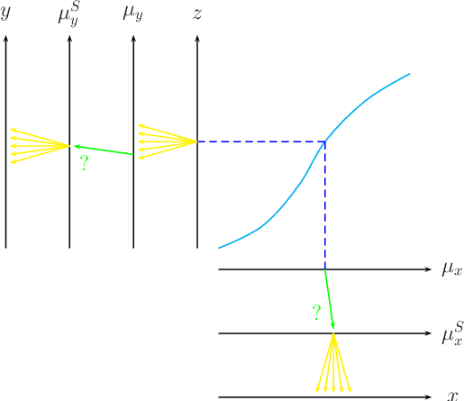
shows the graphical model containing the new ingredients. The links and are to remember that systematics could also effect the error functions. An alternative visual picture of the probabilistic model is shown in Fig. 4. Note the different symbols to indicate the different uncertain processes: the divergent arrows (in yellow, if you are reading an electronic version of the paper) indicate that, given a value of the ‘parent’ variable, the ‘child’ variable fluctuates on an event-by-event basis; the green single arrow with the question mark indicate that, given a value of the ‘parent’, the child will always take a fixed value, though we do not know which one.
Obviously, the practical implementation of complicate systematic effects in complicate fits can be quite challenging, but at least the Bayesian network provides an overall picture of the model. The simplest case is that of linear fit where only offset and scale uncertainty are present, with uncertainty modeled by a Gaussian distribution. This means that the ’s and their uncertainty are as follows ( is the scale factor of uncertain value):
| (83) | |||||
| (84) | |||||
| (85) |
In this case we can get
an hint of how the uncertainty about and change without
doing the full calculation
following an heuristic approach, valid when
is approximately multivariate Gaussian and
the details of which can be found
in Ref. [16]. We obtain the following results,
in which indicates the contribution
to the uncertainty about the slope due to uncertainty
about ,
that due to the scale factor , and so
on77
7
In Ref. [16] is indicated by
, by , and so on.:
| (86) | |||||
| (87) | |||||
| (88) | |||||
| (89) | |||||
| (90) | |||||
| (91) | |||||
| (92) | |||||
| (93) |
All contributions are then added quadratically to the so called ‘statistical’ ones.
9 Conclusions
The issue of fits has been approached from probability first principles, i.e. using throughout the rules of probability theory, without external ad hoc ingredients. It has been that the main task consists in building up the inferential model, that means in fact to properly factorize the joint probability density function of all variables of the problem. We have seen that this factorization, based on the so called chain rule of probability theory, has a very convenient graphical representation, that takes the name of Bayesian (or belief/causal/influence) network. Modeling the problem in terms of such networks not only helps to understand the problem better, but, thanks the huge amount of mathematical developments relates to them, it becomes the only way to get a (numerical) solution when problems get complicated.
We have also seen how to recover well known formulas, obtained starting from other approaches, under well defined conditions, thus indicating that other methods can be seen as approximations of the most general one, and that are therefore applicable if the conditions of validity hold.
The linear case with errors on both axis and extra variance of the data has been shown with quite some detail, giving un-normalized formulas for the pdf. In particular, going to the pretext to write this paper, we can see that Eq. (43) of Ref. [17] is not reproduced. In fact, if I understand it correctly, that equation should have the same meaning of Eq. () of this paper. However, Eq. (43) of Ref. [17] contains an extra factor (using the notation of this paper), that it is a bit odd, for several reasons (besides the fact that I do not get it – but this could be judged a technical argument by the hurry reader). The first reason is just dimensionality: is homogeneous with and for this reason can be combined (quadratically) to , but cannot be added tout court to 1. The second is that if there was such a factor in Eq. (), then one cannot reproduce Eqs. (58), (60) and (61), that one can be obtained in simpler ways (and that give rise to the likelihoods shown in Section 6, some of them rather well known). Note that the addition of a term in Eq. () has the net effect of overestimating , an effect that is consistent with the claim by [1] of a slope larger than that obtained by [14].88 8 As a rule of thumb, since the extra variance of the data of [14] is rather important, the slope has to be very close to that obtained neglecting all and and making a very simple least square regression.
References
- [1]
D.E. Reichart,
Comment on
astro-ph/0507588
and astro-ph/0508483,
astro-ph/0508529. - [2]
G. D’Agostini,
Bayesian reasoning in data analysis:
A critical introduction,
World Scientific Publishing, 2003. - [3] G. D’Agostini, The Fermi’s Bayes Theorem, physics/0509080.
- [4] http://en.wikipedia.org/wiki/Bayesian_network.
- [5] D. Heckerman, A Tutorial on Learning With Bayesian Networks, MSR-TR-95-06, 1995, http://research.microsoft.com/research/pubs/view.aspx?msr_tr_id=MSR-TR-95-06
- [6] F.V. Jensen, Bayesian Networks and Decision Graphs, Springer, 2001.
- [7] R.E. Neapolitan, Learning Bayesian Networks, Prentice Hall, 2003.
- [8] HUGIN Expert, http://www.hugin.com/Products_Services/Products/Demo/.
- [9] F.B Cozman, “JavaBayes version 0.346 – Bayesian networks in Java”, January 2001, http://www-2.cs.cmu.edu/~javabayes/Home/.
- [10] http://www.roma1.infn.it/~dagos/bn/.
- [11]
BUGS,
The BUGS Project - Bayesian inference Using Gibbs Sampling,
http://www.mrc-bsu.cam.ac.uk/bugs/welcome.shtml. - [12] http://www.roma1.infn.it/~dagos/BUGS/.
- [13] C. Andrieu at al., An Introduction to MCMC for machine learning, Machine Learning 2002 (preprint http://www.cs.ubc.ca/~nando/papers/mlintro.ps and mlintro.pdf).
- [14] C. Guidorzi, Testing the GRB Variability/Peak Luminosity correlation using the pseudo-redshifts of a large sample of BATSE GRBs, astro-ph/0508483.
- [15] G. D’Agostini, Asymmetric Uncertainties: Sources, Treatment and Potential Dangers, physics/0403086.
- [16]
G. D’Agostini, Errori e incertezze di misura.
Rassegna critica e proposte per l’insegnamento,
Nota Interna 1094, 1998,
pp. 69-70,
http://www.roma1.infn.it/~dagos/perfezionamento.ps (and pdf),
http://www.roma1.infn.it/~dagos/perfezionamento/node57.html. - [17] D.E. Reichart, Dust extinction curves and LY forest flux deficits for use in modeling GRB afterglows and all other extragalactic point sources, ApJ 553 (2001) 235 (preprint astro-ph/9912368).