On Minimum Violations Ranking in Paired Comparisons

The definition of a ranking of $n$ objects we have used so far is an ordering of the $n$ objects from the first place to the last ($n$-th). More precisely, we assign to each object an integer rank $r_{i}$ ($1\leq r_{i}\leq n$), such that the ranking $\mathbf{r}=\{r_{1},r_{2},\dots,r_{n}\}$ is a permutation of $\{1,\ldots,n\}$. (Although we do not allow ties in a ranking, they can be produced in the final standings if the mean ranks of multiple objects are equal.) We can also visualize this as $n$ objects occupying $n$ ordered slots, which we will call the n-space. This is illustrated in Fig. 2(a) for $n=3$. It will be shown later that it is more convenient to work in a larger N-space, where the same $n$ objects occupy $n$ slots among $N$ ($N\gg n$) ordered slots. The ranking in the N-space is similarly defined as $\mathbf{s}=\{s_{1},s_{2},\ldots,s_{n}\}$, where $s_{i}$ is the label of the slot occupied by object $i$. This is illustrated in Fig. 2(b).

We can define a natural mapping between a ranking in the $n$-space and rankings in the N-space that have the same relative standings of the objects (i.e., in terms of being higher or lower than others), hence the same number of violations. Under this mapping, each ranking in the $n$-space corresponds to exactly ${N\choose n}=N^{n}/n!$ rankings in the $N$-space. Therefore, Fig. 2(a) gets mapped onto Fig. 2(b).

Now, consider an object ranked $r$ in some ranking in the n-space. Its mean rank $\tilde{s}(r)$, averaged over the mapping of the ranking in the N-space, is given by

Numerical studies strongly suggest that $\mathcal{L}(N,n,r)=1+\mathrm{O}(n/N)\to 1$ for $N\gg n$. If this is true (and for all the examples that we will be presenting in the final part of this paper, it is), Eq. (1) tells us that $\tilde{s}(r)$ is identical to $r$ up to a constant prefactor, i.e. $\tilde{s}(r)=r\cdot(N/n+1)\equiv r\cdot C$. Assume that we have a set $R=\{\mathbf{r}^{a},\mathbf{r}^{b},\ldots\}$ of rankings in the n-space (e.g., of all MVRs), and that we are trying to calculate the mean rank $\overline{r_{i}}$ of object $i$ over $R$, which is given by

Thus we can conclude that calculating $\overline{r_{i}}$ over $R$ is equivalent to calculating $\overline{s_{i}}$ over the corresponding rankings in the N-space of $R$ under the mapping. See Fig. 2(c). We will be working exclusively in the N-space from now on.

It is well known that the canonical ensemble formalism greatly facilitates the calculation of physical quantities in a statistical mechanical system such as that of gaseous particles, while giving identical predictions as the microcanonical ensemble formalism. The essence of the canonical ensemble formalism lies in one being flexible on which microstates to include in evaluating the partition function; typically, all states of different energies $E$ are allowed, whereas in the microcanonical formalism only states with a specific energy are allowed Callen 1985.

We will formulate our problem in an entirely analogous fashion: we include all microstates (rankings) of any number of violations (i.e., not just the MVRs) to form an ensemble. As usual, the first step is to assign the probability $P(\mathbf{s})$ to each ranking $\mathbf{s}$. The fairest, most unbiased way to do this is to maximize the entropy

subject to certain constraints given by the mean values of the observables Jaynes 1957; Jaynes 2003. Our observables are the objects’ ranks $\{s_{1},s_{2},\ldots\}$ and the number of violations $V(\mathbf{s})$, which can be written as

where $\Theta(s_{j}-s_{i})\equiv\Theta_{ij}$ is the Heaviside stepfunction. Therefore, the constraints are given as

Using the Lagrange multiplier method on $\mathcal{S}$, we get the following solution for $P(\mathbf{s})$:

where $\vec{\alpha}=\{\alpha_{1},\ldots,\alpha_{n}\}$ and $\beta$ are the Lagrange multipliers, and $H_{0}\equiv-\vec{\alpha}\cdot\mathbf{s}=-\sum_{i}\alpha_{i}s_{i}$ and $H_{2}\equiv-\beta V$ are called Hamiltonians. The normalizing factor $Z$ is the usual partition function, given by

Since we stipulated that all rankings with the same value of $V$ be given equal probability, $P(\mathbf{s})$ of Eq. (6) can be a function of $V$ only. Therefore, all values of $\alpha$ are actually equal to $0$. They are formally retained in Eq. (6) because they will serve as the differentiation variables when calculating $\overline{s_{i}}$ from Eq. (5):

where $F=-\ln Z$ is the free energy. On the other hand, $\beta$ will be a negative real number, as we are trying to minimize (i.e. discourage the formation of) violations. Furthermore, the MVR limit is given by $\beta=-\infty$.

The model is now fully defined. Before we proceed, let us briefly discuss the advantages of having this theoretical model and solutions to it. The first advantage, as mentioned earlier, is that our formulation guarantees a fair sampling of the phase space by definition, whereas exact or heuristic methods merely attempt to find one specific MVR of a paired comparison. The second advantage is that, although Eq. (6) lends itself to Monte Carlo simulations in a straightforward manner (if it can easily be done for $\beta=-\infty$ at all) for numerical results, having an analytical solution by which we can calculate $\overline{\mathbf{s}}$ for any paired comparison would be more convenient, possibly requiring no simulation effort at all.

Eq. (12) tells us that in order to evaluate $Z$ or $F$, we need to calculate $\langle V^{l}\rangle=\langle(\sum_{ij}\Theta_{ij})^{l}\rangle$ (with a tacit understanding that the summation is done over $(i,j)$ for which $A_{ij}=1$).

Let us look at some examples. First, consider $\langle V\rangle$:

Since $\Theta_{ij}$ is equal to $1$ when $s_{i}<s_{j}$ and $0$ otherwise, $\langle\Theta_{ij}\rangle$ is simply equal to the probability that $s_{i}<s_{j}$. We can easily calculate it using Eq. (11):

The validity of this can be checked quickly by noting its limiting value for $\alpha_{i},\alpha_{j}\to 0$, which is ${1\over 2}+\frac{1}{2N}\simeq{1\over 2}$. This is as expected, since if we randomly put two teams at any position with uniform probability (this is what $\alpha\to 0$ means), there will be $\frac{1}{2}$ chance that one will be ranked higher than the other.

Next, consider $\langle V^{2}\rangle=\sum_{ij}\sum_{km}\langle\Theta_{ij}\Theta_{km}\rangle$. We have three types of products $\Theta_{ij}\Theta_{km}$, depending on the relation between $(i,j)$ and $(k,m)$:

1. 1.

   $(i,j)=(k,m)$ so that $\Theta_{ij}\Theta_{km}=\Theta_{ij}^{2}=\Theta_{ij}$, since $\Theta$ is either $1$ or $0$.

2. 2.

   $(i,j)$ and $(k,m)$ share no index, so that $i\neq k,m$ and $j\neq k,m$. We shall call this a disconnected product.

3. 3.

   $(i,j)$ and $(k,m)$ share one index, for example $j=k$ and $i\neq m$. We shall call this a connected product.

Terms of the first kind will sum to $\langle V\rangle$. In the second case, since the positions of $i$ and $j$ are independent of those of $k$ and $m$, we can easily see that $\langle\Theta_{ij}\Theta_{km}\rangle=\langle\Theta_{ij}\rangle\langle\Theta_{km}\rangle$. The third case is more interesting, because $\langle\Theta_{ij}\Theta_{jm}\rangle$ does not factor like the previous case since $\Theta_{ij}$ and $\Theta_{jm}$ are “connected” via $j$. We can see this explicitly by calculating its average in a manner similar to Eq. ():

Its limiting value for $\alpha_{i},\alpha_{j},\alpha_{m}\to 0$ is $\frac{1}{6}$ not $\frac{1}{4}$, as it would have been if the product factored.

Therefore, $\langle V^{2}\rangle$ can be written, schematically, as

The reason for stressing the distinction between disconnected and connected products will become clear in later sections.

Here, let us study the general implication of $\Theta^{2}=\Theta$ on $V^{l}$. Assume that we have applied the rule exhaustively to every term of $V^{l}$. Then $V^{l}$ will have become a linear combination of all possible products of $1,2,\ldots,l$ distinct $\Theta$s, namely,

where $\phi_{k}$ is the sum of all possible products of $k$ distinct $\Theta$’s, and $\{a_{lk}\}$ are appropriate integer coefficients. For example, $V^{3}$ can be written as

The meaning of $a_{lk}$ is clear: it is the number of ways of selecting one $\Theta$ from each $V$ such that the selection of size $l$ includes $k$ distinct types of $\Theta$s. Now, consider a particular set of $k$ distinct $\Theta$s. The number of ways of choosing $l$ elements from the set, without the constraint that each of $k$ types must be present at least once, is simply $k\times k\times\cdots=k^{l}$. This is also the sum of the number of ways that the selection contains $1,2,\ldots,k$ distinct types of $\Theta$ from the set. This leads to the relation $\sum_{m=1}^{k}{k\choose m}a_{lm}=k^{l}$ or, equivalently,

Multiplying each side by $z^{l}/l!$ and summing them over $l=1,2,\ldots,\infty$ gives the recursion relation for its generating function $g_{k}(x)=\sum_{l=1}^{\infty}x^{l}a_{lk}/l!$:

This implies $g_{k}(z)=(\mathrm{e}^{z}-1)^{k}$ by mathematical induction, with the initial condition $g_{1}(z)=\sum_{l=1}^{\infty}z^{l}a_{l,1}/k!=(\mathrm{e}^{z}-1)$ and $a_{l1}=1$. This is the solution to the same result previously reported by us in Park and Newman 2005b.

Since $\phi_{1}=V$, $Z$ of Eq. (12a) now becomes

This looks as if we have replaced $\langle V^{l}\rangle$ and $\beta$ in Eq. (12) with $\langle\phi_{l}\rangle$ and $\eta\equiv(\mathrm{e}^{\beta}-1)$. But what we have here is more than a facelift: thanks to $\eta$, the evaluation of $\langle\phi_{l}\rangle$ up to any finite $l$ gives us an infinite-order expansion in terms of $\beta$. This is analogous to the “partial resummation” in field theory. The MVR limit under this change of variables is $\eta=-1$.

Using Eq. (22), $F_{1}$ of Eq. (12) can also be written as a power series of $\eta$:

where its coefficients $f_{l}$ can be determined by the Taylor series

For example, the first three $f$’s are

Since $\phi_{l}$ is a sum of products of $\Theta$s, this tell us that $F_{1}$ is a linear combination of products of their unperturbed averages. For instance, it has terms made up of powers of $\langle\Theta_{ij}\rangle$: i.e., $\langle\Theta_{ij}\rangle$ from $\langle\phi_{1}\rangle$, $\langle\Theta_{ij}\rangle^{2}$ from $\langle\phi_{1}\rangle^{2}$, and so forth, which all add up to a quantity $\psi[\Theta_{ij}]$. We will call this quantity the contribution of $\Theta_{ij}$ to the free energy Eq. (23):

Similarly, we can define $\psi[\Theta_{ij}\Theta_{km}](\Theta_{ij}\neq\Theta_{km})$, which is the sum of the products of averages of products involving both $\Theta_{ij}$ and $\Theta_{km}$. These are trickier than Eq. (26): we have $\langle\Theta_{ij}\Theta_{km}\rangle$ from $\langle\phi_{2}\rangle$, $\langle\Theta_{ij}\rangle\langle\Theta_{km}\rangle$ from $\langle\phi_{1}\rangle^{2}/2$ in $f_{2}$, $\langle\Theta_{ij}\Theta_{km}\rangle\langle\Theta_{ij}\rangle$ from $\langle\phi_{2}\rangle\langle\phi_{1}\rangle$ in $f_{3}$, and so forth. These add up to give

Before we proceed any further, let us introduce the diagrammatic representation of products of $\Theta$s, shown in Fig. 3. Here, a single $\Theta_{ij}$ is drawn as an arrow pointing to $i$ from $j$ (Fig. 3(a)). A juxtaposition of two or more arrows will be understood as a product of the corresponding $\Theta$s, such as Fig. 3(b) which stands for $\Theta_{ij}\Theta_{jm}$. Note that the diagram for the connected product $\Theta_{ij}\Theta_{jm}$ consists of a single component. In graph theory parlance, such a diagram is also called connected. As a matter of fact, a connected product implies a connected diagram and vice versa in this representation scheme. Examples of connected and disconnected diagrams (i.e., products) of more than two $\Theta$s are shown in Fig. 3(c) and (d).

Therefore, evaluating the free energy $F_{1}$ means calculating $\psi$ of all possible diagrams, and Eqs. (26) and (27) are such calculated up to $\mathrm{O}(\eta^{3})$. However, any power of $\langle\Theta_{ij}\rangle$ can only come from Taylor-expanding the logarithm of $\eta\langle\Theta_{ij}\rangle$ contained in the $\eta\langle\phi_{1}\rangle$ of Eq. (22), we can easily see that $\psi[\Theta_{ij}]$ has to be

Taylor-expanding this to $\mathrm{O}(\eta^{3})$ indeed gives Eq. (26).

The situation is similar for $\psi[\Theta_{ij}\Theta_{km}]$. It could have only come from Taylor-expanding $-\ln\bigl(1+\eta\langle\Theta_{ij}+\Theta_{km}\rangle+\eta^{2}\langle\Theta_{ij}\Theta_{km}\rangle\bigr)$ of Eq. (23), but this also produces powers solely of $\langle\Theta_{ij}\rangle$ or $\langle\Theta_{km}\rangle$, which we now know are $\psi[\Theta_{ij}]$ and $\psi[\Theta_{km}]$. Therefore, we have

Now, assume that $\Theta_{ij}\Theta_{km}$ is disconnected, i.e. $\langle\Theta_{ij}\Theta_{km}\rangle=\langle\Theta_{ij}\rangle\langle\Theta_{km}\rangle$. Then $\psi[\Theta_{ij}\Theta_{km}]$ vanishes. This means that only connected products of two $\Theta$s contribute to the free energy. In fact, this is generally true for products of any number of $\Theta$s: only connected products (diagrams) make nonzero contributions to the free energy. Therefore, Fig. 3(c) contributes; Fig. 3(d) does not.

Now we have an iterative prescription for calculating $\psi$ of any diagram: from the negative of the logarithm of $1$ plus the terms that represent itself and its subgraphs in Eq. (22), subtract the $\psi$’s of the subgraphs. As an example, let us use this rule to evaluate $\psi[\Theta_{ij}\Theta_{km}\Theta_{lq}]$. The subgraphs of $\Theta_{ij}\Theta_{km}\Theta_{lq}$ are $\Theta_{ij}$, $\Theta_{km}$, $\Theta_{lq}$, $\Theta_{ij}\Theta_{km}$, $\Theta_{km}\Theta_{lq}$ and $\Theta_{lq}\Theta_{ij}$. Therefore,

Again, this term vanishes unless $\Theta_{ij}\Theta_{km}\Theta_{lq}$ is connected.

Our strategy is now clear: identify all connected diagrams (composed of up to some desired number of $\Theta$), add up their contributions $\psi$, and perform the differentiation of Eq. () to obtain $\overline{\mathbf{s}}$.

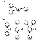
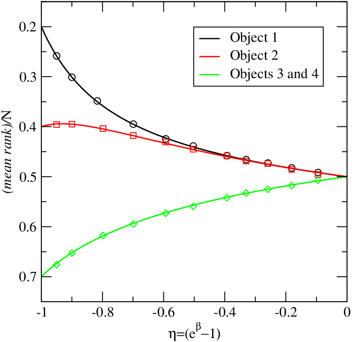
As the first example, take a simple comparison whose adjacency matrix is given in Table 1. It can be visualized as Fig. 5(a). We can intuitively see that object $1$ must be ranked at the top, followed by $2$, while $3$ and $4$ should be tied (since they are topologically indistinguishable) at last to obtain a minimum number of violations ($0$). In order to use our expansion results, we must count the connected subgraphs involving each object, which are shown in Fig. 5(b) for object $1$. After repeating this process for all objects, we obtain the following solutions for $\overline{\mathbf{s}}$:

Since we have considered all subgraphs appearing in Fig. 5(a), these must be exact. An excellent agreement with Monte Carlo simulation results for the entire range of $\eta$ in Fig. 6 confirms this.

A closer inspection of Fig. 6 tells us that the mean ranks are $(N+1)/2=N/2$ for $\eta=0(\beta=0)$ as expected, while $\overline{s_{1}}$ and $\overline{s_{2}}$ begin to diverge noticeably around $\eta=-0.6(\beta=-0.9)$. Since objects $1$ and $2$ are indistinguishable on the first order (they both have a win-loss differential of $1$), this has to be the point where second and third-order diagrams begin to contribute significantly. The MVR solutions at $\eta=-1$ also agree with Eq. (1).

Larger data sets will certainly contain fourth- or higher-order connected diagrams, and therefore our third-order expansion will be an approximation. However, it is still interesting to see how valid our third-order expansion can be as a true approximation. We study this issue with the following examples.

A round-robin tournament is a complete paired comparison. Ali et al. studied the minimum violations ranking problem of the $5$-player round-robin tournament (with ${5\choose 2}=10$ comparisons) using a couple of heuristic methods on the nine distinct configurations they had identified Ali et al. 1986. One of those tournaments (labeled $5$ in their paper) is given in Table 2, and visualized in Fig. 7. The correct MVR standings should be $\{1,2,3,4,5\}$.

Fig. 8 shows the perturbation and Monte Carlo simulation results. We see that there exists a wide range of $\eta$ (between $-0.8$ and $0$) in which the perturbation agrees with the simulation well within $2\%$ of $N$ and predicts the relative standings correctly, whereas closer to $\eta=-1$ it behaves in a haphazard way and gives incorrect standings. This latter behavior is certainly due to the missing higher-order diagrams. We find almost identical behaviors for the eight other tournaments as well: the perturbation solution is stable and predicts correct standings including ties for a wide range of $\eta$, while near $\eta=-1$ it fails.

Compare this to the heuristic methods of Ali et al., which merely succeeds in finding one specific MVR for each the tournament. Furthermore, strangely enough, they regard the emergence of “tied ranks” as an undesirable feature of a method in their study. We believe to the contrary: it is only fair to give tied ranks to topologically indistinguishable players, which our method does explicitly.

As a final example, we consider a large-scale data set mentioned earlier, American collegiate football. In the year $2004$, $117$ universities played a total of $622$ games in the regular season. Ranking of colleges based on the outcomes of those games is of particular interest, because schools ranked high in the ‘‘official’’ ranking (currently determined by a combination of human polls and several computer algorithms) get invited to play in prestigious post-season bowl games, while the top two schools get to play in the national championship game ³³ 3 www.bcsfootball.org. An invitation to these games is not only honorable, but brings practical benefits to the schools, including much publicity through the media, financial compensations worth millions of US dollars, and an increase in applications from prospective students Dunnavant 2004.

Due to the small number of games ($\sim 11$) a school plays in a season compared to the number of possible opponents ($\sim 120$), a simple win-loss differential is a hopelessly insufficient measure of a team’s strength. Therefore, the official computer algorithms as well as the hundreds of rankings schemes devised by the fans of the sport employ various criteria that their inventors or developers deem necessary and important in order to assess the college teams’ strengths Park and Newman 2005a; Keener 1993; Harville 2003; Callagan et al. 2004.

One often evaluates the quality of an algorithm by counting the violations in the final ranking it produces Martinich 2002. Any MVR will perform the best in this respect by definition, but in a recent study of a particular MVR that was mentioned earlier was shown to have performed as well as or better than other ranking methods in other tests as well Coleman 2005. Again, this study was done for one particular MVR, and so it would be an interesting topic for future research to study how $\overline{\mathbf{s}}$ from Eq. () perform in those tests.

In this paper, though, let us concentrate on our third-order perturbation expansion. In Fig. 9 we see that it shows a behavior quite similar to the one we have seen in the previous example: we have a smooth, well-behaved range (though narrower, $-0.3\lesssim\eta<0$), followed by a region of large fluctuations.