Layered Complex Networks
Abstract
Many complex networks are only a part of larger systems, where a number of coexisting topologies interact and depend on each other. We introduce a layered model to facilitate the description and analysis of such systems. As an example of its application we study the load distribution in three real-life transportation systems, where the lower layer is the physical infrastructure and the upper layer represents the traffic flows. This layered view allows us to capture the fundamental differences between the real load and commonly used load estimators, which explains why these estimators fail to approximate the real load.
pacs
89.75.Hc, 89.75.Fb, 89.40.Bb, 89.20.HhThe topologies of the Internet at the IP layer Faloutsos99, of the World Wide Web Albert99 or the
networks formed by Peer To Peer (P2P) applications Adamic01 have recently drawn a lot of attention. These graphs
have been studied separately, as distinct objects. However, they are closely related: each WWW or P2P link virtually
connects two IP nodes. These two IP nodes are usually distant in the underlying IP topology and the virtual connection
is realized as a path found by IP routers. In other words, the graph formed by an application is mapped on the
underlying IP network. Although the topologies at both layers might share a number of statistical properties (such as a
heavy-tailed degree distribution), they are very different.
There exist layers also under the IP layer; even in a simplified view of the Internet we must distinguish at least one
- the physical layer. It consists of a mesh of optical fibers that are usually put in the ground along roads, rails, or
power-lines. This results in topologies very different from those observed at the IP layer. A mapping of the IP graph
onto the physical layer must satisfy a number of constraints (see e.g., Kurant05).
Another important class of real-life systems is transportation networks. The graphs based on the physical infrastructure of such networks were analyzed on the examples of a power grid Watts98; AlbertUSAPowerGrid, railway network Indian03, road networks Gastner04; Rosvall05, or urban mass transportation systems Latora01; Stations04; Gastner04b; Sienkiewicz05. Although this approach often gives a valuable insight into the studied topology, it ignores the real-life traffic pattern and hence captures only a part of the full picture. Interestingly, the networks of traffic flows were studied separately, for instance the flows of people within a city Chowell03, and commuting traffic flows between different cities Montis05. These studies, in turn, neglect the underlying physical topology. A comprehensive view of the system requires to analyze both layers (physical and traffic) together. Of course, a partial knowledge of the traffic pattern could be introduced into the physical graph by assigning weights reflecting the amount of carried traffic to the physical edges. This describes well a specific type of transportation network, where all traffic flows are one-hop long and where the two layers actually coincide, such as airport networks Barrat04; Guimera05. However, in the presence of longer (than one hop) traffic flows, the weighted physical graph is not sufficient. For instance, the failure of a single physical node/edge should affect (delete or cause to reroute) all traffic flows using this edge/node, which requires the knowledge of the traffic graph and of the actual routes of these flows in the physical graph.
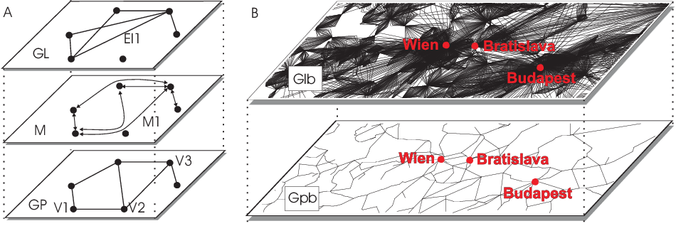
Coexisting and dependent graphs can also be observed in social networks Wasserman94, where the same set of nodes may be connected in various ways, depending on the type of relationship chosen to be represented by edges. These graphs are related to each other. It is common, for instance, to establish a new link in a business relationship graph (e.g., to find a job) by performing a search in our acquaintanceship network (i.e., by asking our friends who ask their friends, etc) Granovetter73. This new direct business link translates into a path in the acquaintanceship network.
The above examples call for the introduction of additional layers to the description of some complex systems. Therefore
we propose a general multi-layered model. We explain it on the example of two layers; all the definitions
naturally extend to any number of layers. In the two-layered model, the lower-layer topology is called physical
graph , and the upper-layer topology is called logical graph . We assume that the sets of nodes at both layers are identical, i.e., , but as a
general rule we keep the indexes and to make the description unambiguous. Let be the number of
nodes, . The physical and logical graphs can be directed or undirected,
depending on the application. The nodes and edges can have weights assigned to them and denoted by ,
with for unweighted graphs. Every logical edge is mapped on the physical graph
as a path connecting the nodes and , corresponding to and
. (A path is defined by the sequence of nodes it traverses.) The set of paths corresponding to all logical
edges is called mapping of the logical topology on the physical topology. Now, the load
of a node
is the sum of the weights of all logical edges whose paths traverse :
| (1) |
In a transportation network is the total amount of traffic that flows through the node ; if the logical graph is unweighted, counts the number of logical edges that are mapped on .
Here, we apply this two-layered framework to study transportation networks. The undirected, unweighted physical graph will henceforth capture the physical infrastructure of a transportation network, and the logical graph will reflect the undirected traffic flows. All data studied in this paper is extracted from timetables of public transportation systems. First, we take a list of all of trains, metros and buses departing in the system within one weekday (time-span of 24 hours). A timetable gives the exact route of each vehicle, which translates directly into a logical edge (connecting the first and the last station) and its mapping . The number of vehicles following the same path in both possible directions defines the flow intensity - the weight of the logical link. (In this context, the logical graph is equivalent to a traffic matrix in transportation science TransportationBook.) We describe the algorithm to extract the two layers and the mapping from timetables in KurantRailwayAlgorithm.

| Dataset | # vehicles | ||||
|---|---|---|---|---|---|
| WA - Warsaw | 1529 | 1827 | 90 | 324 | 26075 |
| CH - Switzerland | 1679 | 1750 | 142 | 539 | 7482 |
| EU - Europe | 6276 | 7273 | 181 | 6623 | 54073 |

We study three examples of transportation networks, with sizes ranging from city to continent. As an example of a city, we take the mass transportation system (buses, trams and metros) of Warsaw (WA), Poland. At a country level, we study the railway network of Switzerland (CH). Finally we investigate the railway network formed by major trains and stations in most countries of central Europe (EU). The basic characteristics of these networks can be found in Table 1 and in Fig. 2. All physical topologies are connected, planar or close to planar, with the diameter in the order of (the diameter of a graph is the length of the longest of all possible shortest paths), and node degree distributions decaying exponentially (the degree of a node is the number of edges incident on this node). These features are common to many physical transportation graphs, such as a road network or a railway system. The logical graphs are strikingly different. They are sparse and have multiple components, among which many isolated nodes. The degree distributions of the logical graphs are right-skewed, meaning that there is a small number of nodes with very high degree. This is confirmed by the almost linear shape of the distribution in the log-log scale plot shown in Fig. 2b; a fully linear shape would indicate a power-law (a heavy-tailed distribution). Similar right-skewed distributions are observed for the weights of edges in the logical graphs (Fig. 2c). In Fig. 2d, we compare the length distribution of real traffic flows with the length distribution of all-to-all shortest paths. The former is very much left-skewed, which means that the real flows tend to be local.
Knowing the topologies and the mapping of both layers, we can easily compute the load of a node with formula (1). For comparison purposes, we present below two load estimators based exclusively on the physical graph . For load estimators we take two metrics known in social networks as centrality measures; they are used to assess the importance of nodes. Our first metric is node degree . It seems natural that the nodes with a high degree carry more traffic than the less connected nodes. Our second metric is betweenness Freeman77. The betweenness of a vertex is the fraction of shortest paths between all pairs of vertices in a network, that pass through . If there are more than one shortest path between a given pair of vertices, then all such paths are taken into account with equal weights summing to one. Betweenness aims at capturing the amount of information passing through a vertex. Indeed, many authors take betweenness as a measure of load either directly Goh01; Holme02; Motter02; Szabo02; Bollobas04; Zhao04, or with slight modifications AlbertUSAPowerGrid; Moreno04; Tadic04
In Fig. 3 we compare the distribution of the real load with its two estimators: node degree and betweenness. The geographical patterns formed by the three metrics differ substantially (see Fig. 3abc). To quantify these differences, in Fig. 3d we present the scatter plots of these two estimators versus the real load . The correlations between them are very low, which is confirmed by low values of the corresponding Pearson’s coefficients (top left corner of every plot). For instance, for the value of load , the corresponding values of betweenness cover more than two orders of magnitude. Surprisingly, contrary to the commonly admitted view, the node degree approximates the real load better than betweenness.
Why do load estimators fail to mimic the real load pattern? Are there some fundamental reasons behind this? The layered
view of the system is very helpful in answering these questions. First, observe that the ways we compute node degree,
betweenness and real load, can be unified by recasting the first two in the two-layered setting. Indeed, both the node
degree and the betweenness can be computed as the node load (1) in two-layered systems with specific
logical topologies mapped on the physical graph using shortest paths. We denote these specific logical graphs
by and , for the node degree and the
betweenness , respectively. They are defined as follows.
In the case of the node degree, pick : the logical graph is identical to the physical
graph . Hence the mapping of on reduces trivially to single hop traffic
flows, and (1) boils down to .
For the betweenness, is an unweighted and complete (fully connected) graph. Indeed, the
definition of betweenness requires to find shortest paths between every possible pair of vertices. Note that the
mapping defined by betweenness splits the path (and its weight) if there are more than one shortest path, whereas the
shortest-path mapping simply returns one of them. However, in large graphs this difference is negligible, especially if
the shortest-path algorithm picks one of the possible paths at random.
The same two-layered methodology can therefore be used to compute node degree, betweenness and real load. Moreover, in
all three cases we use the same physical graph and a mapping that follows the shortest path 11
1
The real-life flows almost always coincide with shortest paths connecting their end-nodes.. Consequently, all the
differences between the three metrics are completely captured by the logical graphs ,
and . We compare them in Table 2. The
graph is moderately dense, planar, unweighted, with the degree distribution decaying
exponentially. The edge length, counted in the number of hops in the mapping of this edge, is equal to one for all
edges of . In contrast, the graph is an unweighted and complete graph,
which means it is very dense, with every node of degree equal to . In we find both
short and long edges; their distribution is bell-shaped, as shown by the “all-to-all” curve in Fig. 2d.
Finally, the real-life logical graph is sparse, weighted and has rather local edges (see the “real” curve
in Fig. 2d). Moreover, the node degree and edge weight distributions of are both very much
right-skewed.
| Property |
![[Uncaptioned image]](0510194v1/planar.png)
|
![[Uncaptioned image]](0510194v1/complete.png)
|
![[Uncaptioned image]](0510194v1/scalefree.png)
|
|---|---|---|---|
| Planar | Yes | No | No |
| Weights | = 1 | = 1 | Right-skewed |
| Degrees | Exponential | Right-skewed | |
| Edge lengths | = 1 | Bell-shaped | Exponential |
There are thus a number of fundamental differences between the three logical graphs , and . They explain why the node degree and betweenness fail to mimic the real load distribution. We expect to observe similar differences in other fields. For instance, the logical graph representing the traffic in the Internet shares many properties with the logical graphs of transportation systems studied here. In particular, in the Internet, the distribution of intensity of traffic flows (which is, in this paper, equivalent to the edge weights in the logical graph) was shown to be heavy-tailed Elephants; Meiss05. This is known in the field as “the elephants and mice phenomenon” Elephants, where a small fraction of flows is responsible for carrying most of the traffic. Moreover, the number of flows originating from a given node (which is, in this paper, equivalent to the node degree in the logical graph), was also shown to follow a power-law distribution Meiss05.
To summarize, we have introduced a framework for studying complex systems in which we distinguish graphs on two or more layers. We have shown on the example of transportation networks how the layered view can facilitate the description, comparison and analysis of such systems. Our work represents only a fraction of the possibilities in this area. For example, the layered perspective can completely change our view of the error and attack tolerance of considered systems. It would be also interesting to study how the properties of the topologies at different layers affect the interactions between the layers.
References
- (1) M. Faloutsos, P. Faloutsos, and C. Faloutsos. On power-law relationships of the internet topology. Proc. of ACM SIGCOMM, 1999.
- (2) R. Albert, H. Jeong, and A.-L. Barabási. Diameter of the world wide web. Nature, 401:130–131, 1999.
- (3) Lada A. Adamic, Rajan M. Lukose, Amit R. Puniyani, and Bernardo A. Huberman. Search in power-law networks. Phys. Rev. E, 64:046135, 2001.
- (4) M. Kurant and P. Thiran. On Survivable Routing of Mesh Topologies in IP-over-WDM Networks. Proc. of Infocom’05, 2005.
- (5) D. J. Watts and S. H. Strogatz. Collective dynamics of “small-world” networks. Nature, 393:440–442, 1998.
- (6) Reka Albert, Istvan Albert, and Gary L. Nakarado. Structural vulnerability of the north american power grid. Phys. Rev. E, 69:025103(R), 2004.
- (7) Parongama Sen, Subinay Dasgupta, Arnab Chatterjee, P. A. Sreeram, G. Mukherjee, and S. S. Manna. Small-world properties of the Indian railway network. Phys. Rev. E, 67:036106, 2003.
- (8) Michael T. Gastner and M. E. J. Newman. The spatial structure of networks. cond-mat/0407680, 2004.
- (9) M. Rosvall, A. Trusina, P. Minnhagen, and K. Sneppen. Networks and cities: An information perspective. Phys. Rev. Lett., 94:028701, 2005.
- (10) V. Latora and M. Marchiori. Efficient behavior of small-world networks. Phys. Rev. Lett., 87:198701, 2001.
- (11) Katherine A. Seaton and Lisa M. Hackett. Stations, trains and small-world networks. Physica A, 339:635, 2004.
- (12) Michael T. Gastner and M. E. J. Newman. Shape and efficiency in spatial distribution networks. cond-mat/0409702, 2004.
- (13) J. Sienkiewicz and J. A. Hołyst. Statistical analysis of 22 public transport networks in poland. physics/0506074, 2005.
- (14) G. Chowell, J. M. Hyman, S. Eubank, and C. Castillo-Chavez. Scaling laws for the movement of people between locations in a large city. Phys. Rev. E, 68:066102, 2003.
- (15) Andrea De Montis, Marc Barthélemy, Alessandro Chessa, and Alessandro Vespignani. The structure of inter-urban traffic: A weighted network analysis. physics/0507106, 2005.
- (16) A. Barrat, M. Barthélemy, R. Pastor-Satorras, and A. Vespignani. The architecture of complex weighted networks. Proc. Nat. Acad. Sci. USA, 101(11):3747, 2004.
- (17) R. Guimerà, S. Mossa, A. Turtschi, and L.A.N. Amaral. The worldwide air transportation network: Anomalous centrality, community structure, and cities’ global roles. Proc. Natl. Acad. Sci. USA, 102:7794, 2005.
- (18) Stanley Wasserman and Katherine Faust. Social Network Analysis. Cambridge University Press, Cambridge, 1994.
- (19) M. Granovetter. The strength of weak ties. American Journal of Sociology, 78(6):1360–1380, 1973.
- (20) William R. Black. Transportation. A Geographical Analysis. The Guilford Press, New York, London, 2003.
- (21) M. Kurant and P. Thiran. Extracting the traffic flows and the physical graphs from timetables. physics/0510151, 2005.
- (22) L. C. Freeman. A set of measures of centrality based on betweenness. Sociometry, 40:35, 1977.
- (23) K.-I. Goh, B. Kahng, and D. Kim. Universal behavior of load distribution in scale-free networks. Phys. Rev. Lett., 87(27):278701, December 2001.
- (24) Adilson E. Motter and Ying-Cheng Lai. Cascade-based attacks on complex networks. Phys. Rev. E, 66:065102(R), 2002.
- (25) G. Szabó, M. Alava, and J. Kertósz. Shortest paths and load scaling in scale-free trees. Phys. Rev. E, 66:026101, 2002.
- (26) B. Bollobás and O. Riordan. Shortest paths and load scaling in scale-free trees. Phys. Rev. E, 69(3):036114, March 2004.
- (27) L. Zhao, K. Park, and Y.-C. Lai. Attack vulnerability of scale-free networks due to cascading breakdown. Phys. Rev. E, 70:035101(R), 2004.
- (28) P. Holme and Beom Jun Kim. Vertex overload breakdown in evolving networks. Phys. Rev. E, 65:066109, 2002.
- (29) P. Echenique, J. G. Gardenes, and Y.Moreno. Improved Routing Strategies for Internet Traffic Delivery. Phys. Rev. E, 70:056105, 2004.
- (30) B. Tadić, S. Thurner, and G. J. Rodgers. Traffic on complex networks: Towards understanding global statistical properties from microscopic density fluctuations. Phys. Rev. E, 69(3):036102, March 2004.
- (31) M. Meiss, F. Menczer, and A. Vespignani. On the lack of typical behavior in the global web traffic network. Proc. of WWW2005, 2005.
- (32) D. Papagiannaki, N. Taft, S. Bhattacharyya, P. Thiran, K. Salamatian, and C. Diot. A pragmatic definition of elephants in internet backbone traffic. Proc. of Internet Measurement Workshop, 2002.