Averaging methods for stochastic dynamics of complex reaction networks:
description of multi-scale couplings

Chemical reaction networks are systems of molecular species of different types interacting with each other by means of multiple reactions FeinbergChemNetworks95. In classical chemical systems, the volume of the reactor and population numbers of species of each types are usually large giving the accurate description of the system in terms of the concentrations. Reactors with complex chemistry give rise to complicated systems of nonlinear equations for the concentrations of chemical species that do not lend themselves to analytic solution. Dynamics of these quantities can be modeled via sets of ordinary differential equations (ODEs) which are powerful tools for predicting the dynamical behavior of macroscopic chemical mixtures.

There is a recent renewal of interest in stochastic modeling of chemical systems which came with the recent realization of importance of noise in cellular information processing. At the level of a single cell, number of molecules involved in some processes can be very small and concentrations are described as nano-molar McAdamsArkin97; Oudenaarden02. In addition to that, different processes are also characterized by significantly different times scales ErbanOthmer2005.

Presence of this time-scale separation and highly different copy numbers of molecular species usually complicates the study of biological processes with computer simulations. There is an obvious need for computationally tractable stochastic models on a macro-scale that can provide insights into joint, qualitative, effects arising from interaction of several sub-networks. In deterministic systems of ordinary differential equations, time-scale separation is usually related to the concept of stiffness. It is obviously hard to define the same concept in case of the stochastic systems RathinamGillespie2003.

In spite of these obvious complications some progress has been made in modeling of biochemical networks which express the separation of time-scales. One difficulty is heterogeneity of simulation techniques used for simulation of ODEs/SDEs and stochastic simulation algorithm. One strategy exploited in the literature GillespieTau; RathinamGillespie2003 is based on grouping together of reaction events taking place in a single reaction channel in a fast succession and applying diffusion approximation EthierKurtzBook. In CVRaoArkin2003 Rao et.al. discuss a computational approach for performing elimination of the fast species based on rapid equilibrium in the limit of the infinite time-scale separation. This method was termed quasi-steady state approximation (QSSA). A somewhat similar approach is taken in HaseltineRowlings2002. Formally, this method stems from the classical deterministic QSSA applied to the chemical master equation itself rather then to the (stochastic) differential equation underlying the dynamics of the state vector (numbers of molecular species). The method developed by Cao et al. in CaoGillespiePetzold2005 can be viewed as generalization of approach of Rao et.al. CVRaoArkin2003 but still have the limitations of being derived through the application of deterministic techniques and assumptions to the chemical master equation. It also assumes that averaging procedure can be done by solving the system of algebraic equations for the expectations of the fast variables given slow, termed in CaoGillespiePetzold2005 as a virtual fast process. We note here that studies of stochastic dynamics of diffusion-type processes evolving on different time scales were pioneered by Bogolubov, Khasminski and Freidlin and we refer the reader to monographs FreidlinWentzelBook; GihmanSkorohodSDE; SkorohodAsymptoticSDE.

This paper has two purposes. First, we present the formulation of stochastic reaction dynamics of reaction network consisting of two subnetworks. Compared to many previous results, where usual description of stochastic reaction dynamics follows the approach based on chemical master equation (CME), current publication follows the path-sampling approach and represents the dynamics as a jump-type stochastic differential equations (SDEs).

Second purpose is to provide rigorous procedure for the renormalization of the transition rates of slow reactions in the presence of fast ones. Following the picture of the stochastic dynamics developed in the first part of this paper, we outline the main guidelines for use of stochastic averaging principle including error control analysis. Despite of the recent rebirth of interest to the method of stochastic averaging in applications to stochastic chemical kinetics, very few examples deal with situations when this procedure might break down. We demonstrate here, in a constructive way, how to perform the averaging over fast reaction events and how to obtain the effective slow-scale transition rate.

Organization of this paper is as follows. In the next section we discuss the general probabilistic framework for stochastic dynamics of reaction networks and introduce a scheme for the partition of species and reactions. In Section III we investigate the consequences of possible time-scales separation and present a procedure based on renormalization of transition rates. We also put emphasis on error analysis, outlining main sources of the numerical error on different steps of the procedure. Our paper will end with discussion of examples.

We begin our discussion with a general set-up, introducing basic concepts and notation.

Assume that a well mixed, isothermal system has $S$ different molecular species indexed by $i=1\ldots S$ and there are $R$ reaction channels, index by $r=1\ldots R$, transforming the molecualr composition of these species. For the basic notation and examples we direct reader to DTGillespieBook; GillespieSSA. State vector of the system can be represented as following:

where fist part of the state vector ${X}_{i}\in\mathbb{Z}_{+},i=1\dots S_{X}$ represents main species while the second part ${Z}_{i}\in\mathbb{Z}_{+},i=1\dots S_{z}$ represents intermidiate species $Z_{i},i=1\dots S_{Z}$. Total number of all types of species: $S_{X}+S_{Z}=S$. Vectors $\boldsymbol{\nu}^{X}_{r}$, $\boldsymbol{\nu}^{Z}_{r}$ and $\boldsymbol{\nu}^{XZ}_{r}$ are stoichiometric changes of components ${\bf X}$ and $\boldsymbol{Z}$ if reaction event $r$ takes place. We will not make any assumptions about actual number of molecular species of each type, i.e. we will not assume low or large copy numbers.

We assume, however, that there are three subsets of reactions in the system:

(i) reactions which transform only species $\mathbf{X}$ (we denote this subset $\mathcal{R}_{1}$),

(ii) reactions which transform only species $\boldsymbol{Z}$ (subset $\mathcal{R}_{2}$)

(iii) ”linker” reactions which mix species $\mathbf{X}$ and $\mathbf{Z}$ (subset $\mathcal{R}_{3}$).

Each reaction channel can be specified by the transition rates $a_{r}$ (a positive function) which describes the probability $a_{r}dt$ of reaction event to take place in the interval of time $dt$. Transition rate $a_{r}$ can be further specified as positive functions of $\mathbf{X}$, $\boldsymbol{Z}$, or,in general, on both components $\mathbf{X}$ and $\boldsymbol{Z}$. Based on the definition of subsets $\mathcal{R}_{1,2,3}$ we have:

We do not assume specific dependence of $a_{r}(\cdot)$ on the state variables $\mathbf{X}$ and $\boldsymbol{Z}$ but usually, in the framework of mass action kinetics, it is a product of kinetic rate $k_{r}$ and function $h_{r}(\cdot)$ which represents the number of reactive configurations available at a given state $\mathbf{X},\boldsymbol{Z}$ DTGillespieBook.

There exist different methods to characterize the stochastic chemical dynamics. One of the most popular approach is to provide an equation for the joint probability density $p_{t}(\mathbf{X},\boldsymbol{Z})$, which gives all information about instantaneous state of the system at generic moment of time $t$. Such equation is known as chemical master equation (CME) vanKampen92; DTGillespieBook and it has been intensively described and utilized in recent literature CaoGillespiePetzold2005; CVRaoArkin2003; HaseltineRowlings2002. But even if we can obtain SamoilovCME the solution of CME, which is usually a very hard problem even for simple chemical networks, this approach still have certain limitations, coming from instantaneous description provided by the density $p_{t}(\cdot)$.

To describe the stochastic dynamics of the chemical network one can introduce the set of independent point processes $N_{r}(t),N_{r}(0)=0$ representing the numbers of reaction events which took place in channels $r\in\mathcal{R}$ up to time $t$ and use the mass balance relations:

where vectors $\boldsymbol{\nu}^{Z}_{r},\boldsymbol{\nu}^{X}_{r}$ and $\boldsymbol{\nu}^{XZ}_{r}$ describe the composition change of the system due to the reaction event in the channel $r$. Average number of reaction events in each reaction channel $r\in\mathcal{R}_{1,2,3}$ during the small time interval $[t,t+\delta t)$ are proportional to the transition rates (2):

Processes $N_{r}(t)$ can be considered as time-changed, unit-rate independent Poisson processes $\Pi_{r}(t)$ EthierKurtzBook:

The time change generates path-dependent or self-affecting point processes whose dynamics depend on the information generated by the arrivals of the process $(\mathbf{X}_{t},\boldsymbol{Z}_{t})$ . It is important to take into account that the stochastic differential equation does not only introduce the probability distribution for the pair $(\mathbf{X},\boldsymbol{Z})$ but also generates a measure on the paths, which contains much more information. For almost any realization of the set of $1\ldots R$ standard Poisson processes, $\Pi_{r}(t,\omega)$, parametrized by the element $\omega$ of event space KaratzasShreveBook; EthierKurtzBook and any deterministic initial condition the solution $(\mathbf{X}(t,\omega),\boldsymbol{Z}(t,\omega))$ is a step-wise stochastic process.

Note also, that dynamics of each component $\mathbf{X}$ or $\boldsymbol{Z}$ is non-Markovian if considered separately but the dynamics of the pair $(\mathbf{X},\boldsymbol{Z})$ is Markovian.

So far we have introduced only the basic notation: quite generic system of SDEs given by (3) outlined in this section have not invoked any assumptions on particular relations between different transition rates $a_{r}$ and was totally based on prior information about existence of two groups of species, i.e. $X_{i}$ and $Z_{i}$ which uniquely identified the partition of the reactions into the subsets $\mathcal{R}_{1},\mathcal{R}_{2}$ and $\mathcal{R}_{3}$ .

In the next section we consider the particular implication of time-scale separation including the extensions of the stochastic averaging principle and diffusion approximation.

In many situations, dynamics of main species $\mathbf{X}$ is propagated via large number of fast transitions which transform mainly intermediate species $\boldsymbol{Z}$. One usually desires to construct an approximate, time coarse-grained model, which involve only main species. It is important that approximate problem describes the dynamics of the system on a large time scale and thus is more advantageous for performing simulations without significant sacrifice in accuracy. This section deals with substitution of the original problem with approximate one and demonstrates the form convergence of the approximation under certain assumptions.

We assume that at certain region of state space the following assumption can be made about transition rates $a_{r}(\cdot)$:

where separation of the time-scales is introduced via the small parameter $\epsilon\ll 1$. Problems of this type are challenge for direct application of Stochastic Simulation Algorithm (SSA) BortzKalosLebowitz75; GillespieSSA because they will require the time steps of the order $O(\epsilon)$ with a total computational cost of order $\epsilon^{-1}$. If we want to advance through the time interval $[0,t],~t\sim O(1)$ most of the simulation time will be spent on simulation of reaction events with the high intensity ($\sum_{r\in\mathcal{R}_{2}}a_{r}\propto O({\epsilon}^{-1})$). We would like to find an effective transition rates $\bar{a}_{r}(\cdot)$ for the ”linker” reactions (subset $\mathcal{R}_{3}$), which describe the transition events of the slow reactions ”coarse-grained” over the possible events corresponding to the reaction events in subset $\mathcal{R}_{2}$.

It is instructive to consider a simple reaction scheme involving three species $\mathsf{X}_{1},\mathsf{Z}_{1,2}$ similar to one considered in CaoGillespiePetzold2005:

where rates $k_{1,2}\propto\epsilon^{-1}$ are parametrized by small $\epsilon$ and $k_{3}\propto O(1)$. In this case reactions $\mathsf{Z}_{1}{\rightleftharpoons}\mathsf{Z}_{2}$ forms the subset $\mathcal{R}_{2}$ while reaction $\mathsf{Z}_{2}{\rightarrow}\mathsf{X}_{1}$ corresponds to the subset $\mathcal{R}_{3}$ and subset $\mathcal{R}_{1}$ is empty,i.e $\mathcal{R}_{1}=\{\emptyset\}$. Then systems of equations for components $(X_{1},Z_{1},Z_{2})$ is the following one:

Presence of the scaling factor $\epsilon^{-1}$ in reaction constants $k_{1,2}\epsilon^{-1}$ allows us to consider family of solutions parameterized by $\epsilon$. We expect $Z_{1,2}$ to follow adiabatically the $X_{1t}$. To make that apparent, one can apply the functional law of large numbers to the processes $N_{2,3}(t)$ in time interval $[0,t]$ (see Eqn. (5a)):

where $W_{2,3}(\cdot)$ are two independent Wiener processes EthierKurtzBook. Since parameter $\epsilon^{-1}$ is large, we can conclude that difference

also converges to zero for times $t\leq\ \epsilon/(k_{2}+k_{3})$ in the limit of small $\epsilon$, and we can conclude that:

This means that variables $Z_{1t}$ and $Z_{2t}$ reach a stationary binomial distribution:

on the time scale $t\propto O(\epsilon)$ while sum $Z_{1t}+Z_{2t}$ changes on the much larger time-scale $t\geq O(1)$:

By exploiting the separation of time-scales using the stationary distribution $\pi^{\epsilon}(Z_{1},Z_{2}|X_{1})$ one can replace dynamical quantities $f(Z_{1t},Z_{2t},X_{1t})$ averaged on the time interval $[0,t],\quad~\frac{\epsilon}{k_{2}+k_{3}}\ll t<\frac{1}{k_{1}}$ with their conditional averages:

and eliminate fast variables $Z_{1,2}$ from the description even though the total number of molecules $Z_{1}+Z_{2}$ may be not a large quantity. Thus, taking $f(\cdot)$ to be the ”linker” transition rates $a_{r}(\mathbf{X},\boldsymbol{Z}),~r\in\mathcal{R}_{3}$ one obtains averaged transition rates $\bar{a}_{r}(\mathbf{X})$ which now depend only on the slow variable $\mathbf{X}$. Results of the large deviation theory FreidlinWentzelBook demonstrate weak convergence bounds of the original problem with small but non-zero $\epsilon$ to the solution of the averaged system. But as we mentioned it before, one of the goals of this publication is to analyze and extend averaging process to the situation when $\epsilon$ may be small, but not ’infinitesimally’ small. In the next section III.1 we will try to answer this question.

Given the renormalized survival probabilities and transition rates at different points of state space of main species $\mathbf{X}$:

stochastic dynamics of the main species $X$ can be formulated in the straightforward way, similar to the stochastic simulation algorithm (SSA) GillespieSSA; DTGillespieBook. At the time point $t=0$ state $\mathbf{X}_{0}$ we consider an overall survival probability:

and define a jump moment of the slow process as a first time $\tau_{1}$ when $S(t|\mathbf{X}_{0})$ crosses the value $u$, where the last one is a random number uniformly distributed on the interval $(0,1)$ MHADavisBook:

Post-jump transition kernel is defined by the vector of transition probabilities

i.e. reaction event $r^{*}\in\mathcal{R}_{1,3}$ is selected based on the vector $q_{r}$ and current state is updated:

Then the same procedure is performed starting at the state $\mathbf{X}_{\tau_{1}}$ with generation of the interval $\tau_{2}$ from the survival probability $S(t|\mathbf{X}_{\tau_{1}})$ and new state $\mathbf{X}_{\tau_{1}+\tau_{2}}$ and so on. As a result one obtains a coarse-grained trajectory:

Question about the overall accuracy and the error control is a delicate question. Below we decompose the overall error of the method it into the following main factors:

1. 1.

   Error in approximating by coarse grained dynamics:

   $$e_{1}=\sup_{0\leq t\leq T}\mathbb{E}(|\mathbf{X}_{t}-\bar{\mathbf{X}}_{t}|^{2})$$

   assuming that transition rates $\bar{a}_{r}(\cdot)$ can be obtained without error.

2. 2.

   Approximation and Monte Carlo error $e_{2}$ of $\bar{a}_{r}(\cdot)$ via the finite number of samples representing the dynamics of $\boldsymbol{Z}_{t}$ at fixed ${\bf X}$.

Below we discuss step by step leading terms in $e_{1},~e_{2}$.

Estimation of the error $e_{1}$ is related to the answer on the following question: what possible error is introduced while performing averaging of rates of reactions in the subsets $\mathcal{R}_{1,3}$ at fixed $\mathbf{X}$?

It is not hard to see that this error is proportional to the probability of the event that minimal jump time over the reactions in group $\mathcal{R}_{1}\cup\mathcal{R}_{2}$ is smaller then $t$ while the minimal jump-time of reaction in the group $\mathcal{R}_{3}$ is larger then $t$:

where average $\langle\ldots\rangle_{X}$ is taken over trajectories $\mathbf{X}^{z}_{t}$ at fixed $\mathbf{Z}$ It is not hard to see that this probability is exponentially small, i.e. $\propto\exp(-{\epsilon}^{-1}\frac{t}{const})$ in the limit $\epsilon\to 0$.

Error $e_{2}$ depends on the number of cumulants we have included in Eqn. (19) and cumulant of order $m$ usually gives contribution proportional to $\epsilon^{m}$. In Appendix we outline the exact method for calculation of the renormalized survival probability based on eigenvalue decomposition of certain linear operator which is a practical approach in situations when state space of the variable $\boldsymbol{Z}$ is not very large.

We now present a simple intuitive example to show that exponential or non-exponential structure of the averaged survival probability is governed by the relationship between time-scales of ”fast” and ”slow” species. Assume that for some reaction channel

rate $a_{r}(X,Z)=k_{r}h_{r}(X)h^{\prime}_{r}(Z)$ jumps reversibly between two values $a_{r}({X},0)$ and $a_{r}({X},1)$ with the stochastic dynamics of $Z_{t}$ governed by simple master equation:

Equation (32) describes the switching transitions between the two states $0$ and $1$. Assuming that state of variable $Z$ is prepared according to the equilibrium density $\pi=(\pi_{0},\pi_{1})=(\frac{k_{10}}{k_{01}+k_{10}},\frac{k_{01}}{k_{01}+k_{10}})$. the average survival probability $\langle e^{-\int_{0}^{t}a_{r}(X,Z^{x}_{t^{\prime}})dt^{\prime}}\rangle$ can be obtained as follows (see also Appendix section for the general computational framework):

This result is very similar in nature to the result obtained in AgmonHopfield83 for the case of identical transition rates. Remarkable and simple result outlined by Eqn. (33) allows us to capture in essence regimes corresponding to the different ratios of the time-scales: $a_{r}\ll(k_{10}+k_{01})$ and $a_{r}\geq(k_{10}+k_{01})$. First regime ($a_{r}\ll(k_{10}+k_{01})$) corresponds to the situation when transitions between different states of $Z$ happens much faster then the average rate $a_{r}(X,0),a_{r}(X,1)$ of the ”linker” process and represents the mean-field (MF) regime. In this case dependence of $ln(S_{r}(t))$ on time $t$ can be very well characterized as linear Fig. 2. Not surprisingly, other regime, i.e. $a_{r}\gg(k_{10}+k_{01})$ can be characterized as gated: in this case effective transition rate $\bar{a}_{r}$ is characterized by the rate of switching of $Z$: $k_{01}+k_{10}$.

Figure 3 demonstrates influence of the second order correlation correction Eqn. (25): $\Delta\bar{a}_{r}(t,\mathbf{X})=\pi_{1}\pi_{0}\frac{t}{\kappa}(1-\frac{\kappa}{t}(1-e^{-\kappa t})),~\kappa=k_{01}+k_{10}$ which fluctuation correction to the effective rate $\bar{a}_{r}(\cdot)$

Dependence of survival probability $S_{r}(t|\mathbf{X})$ in the example of a two-state system can be shown to be non-exponential on the longer time scale but $\ln(S_{r}(t))$ behaves linearly with time at small times $t\leq 1/a_{r}(X,\cdot)$.

Interesting case of non-exponential relaxation kinetics, and specifically non-exponential kinetics at small times can be presented by the following example. Consider a fast reaction given by the dimerization reaction:

and a ”linker” process is described by the relaxation rate depending on the number of dimers $X$ in the following way:

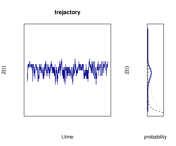
Current value $X$ serves as an activation threshold: at small values of $X$ ($X\propto 1$) only small values of $Z$ contribute to the effective rate but probability that $Z$ takes values away from its average are exponentially suppressed (Fig. 4). On the contrary, if $X$ is large i.e. $X\approx\sum_{Z}\pi(Z|X)Z$ then rate given by Eqn. (36) depends on the typical value of $Z$ and $S_{r}(t|X)$ manifests time dependence similar to the previous example. One can see that this relaxation process shows non-exponential time dependence at small times due to the fact that process $Z_{t}$ rarely visits the states contributing to the maximum of the relaxation rate given by Eqn. (36). We investigate the dependence of the averages survival probability on the level of activation threshold $X$ and value of the equilibrium constant $K_{eq}$. Results presented on the Fig. 5 show non-exponential behavior of averaged survival probability for the system at small times $t$. It is evident that non-exponential behavior of $S_{r}(t|X)$ is less pronounced for large values of $X(~X\approx\langle Z\rangle)$.

Eigenvalue-eigenvector decomposition and calculation of expansion coefficients was performed via standard routines of LAPACK library available at http://www.netlib.org .

Let us summarize the main aspects of this paper. We have studied reduction approach to eliminate a fast intermediate in the chemical reaction network. To develop this method it is important to consider the time coarse-grained transition rates. We have discussed the limitations of the principle of stochastic averaging and its possible extensions through the rigorous technique for construction of the effective transition rates. We outline the procedure for re-normalization of the transition rates and construction of the effective Markov chain for the slow reactions. The merit of the present approach is that it is based on a conceptually transparent probabilistic approach involving the waiting-time distribution.Technique itself resembles a non-Markovian generalization of the Kubo-Anderson theory of stochastic modulation. Our study clearly indicates importance of details of the statistical structure of averaging process.

Author thanks A. Alekseyenko for stimulating discussion on the subject of this publication, T. Ham for valuable suggestions. Author would like to acknowledge DARPA grant # BAA-01-26-0126517 and Prof. A.P.Arkin for support during the course of this research.

References

- [1] M. Feinberg. The existence and uniqueness of steady states for a class of chemical reaction networks. Archive for Rational Mechanics and Analysis, 132:311–370, 1995.
- [2] H. H. McAdmas and A.P. Arkin. Stochastic mechanisms in gene expression. PNAS, 94(3):814–819, 1997.
- [3] E. Ozbudak, M. Thattai, and I. Kurtserand A. D. Grossman a nd A. van Oudenaarden. Regulation of Noise in the Expression of a Single Gene. Nature Genetics, 31, 2002.
- [4] R. Erban and H. G. Othmer. From signal transduction to spatial pattern formation in E. Coli: A paradigm for multiscale modeling in biology. Multiscale Model. Simul., 3(2):362–394, 2005.
- [5] M.Rathinam, L. R. Petzold, Y. Cao, and D. T. Gillespie. Stiffness in stochastic chemically reacting systems: The implicit tau-leaping method. J. Chem. Phys., 119:12784–12794, 2003.
- [6] D.T. Gillespie. The Chemical Langevin equation. J. of Chem. Phys., 113(1):297–306, 2001.
- [7] S. Ethier and T. Kurtz. Markov Processes: Characterization and Convergance. John Wiley & Sons, 1986.
- [8] C. V. Rao and A. P. Arkin. Stochastic chemical kinetics and the Quasi-Steady-State assumption: Application to the Gillespie algorithm. Journal of Chemical Physics, 118(11):4999–5010, 2003.
- [9] E. L. Hasiltine and J.B. Rawlings. Approximate simulation of coupled fast and slow reactions for stochastic chemical systems. J. Chem. Phys., 117(15):6569–6969, 2002.
- [10] Y. Cao, D. T. Gillespie, and L. R. Petzold. The slow-scale stochastic simulation algorithm. J. Chem. Phys., 122:014116, 2005.
- [11] M.I. Freidlin and A.D. Wentzel. Random Perturbations of Dynamical Systems. Springer,New York, 1984.
- [12] I.I.Gihman and A.V.Skorohod. Stochastic Differential Equations. Springer Verlag, 1972.
- [13] A.V.Skorohod. Asymptotic Methods in the Theory of Stochastic Differential Equations. AMS, 1989.
- [14] D.T. Gillespie. Markov Processes: An Introduction for Physical Scientists. Academic,San Diego, 1992.
- [15] D.T. Gillespie. Exact simulation of coupled chemcial reactions. J. of Phys. Chem., 81(25):2340–2361, 1977.
- [16] N.G. van Kampen. Stochastic Processes in Physics and Chemistry. North-Holland Pub. Co., 1992.
- [17] M. Samoilov and John Ross. One-dimensional chemical master equations: Uniqueness and analytical form of certain solutions. Journal of Chem. Phys., 102(20):7983–7987, 1995.
- [18] I. Karatzas and S. E. Shreve. Brownian Motion and Stochastic Calculus. Springer-Verlag, 1988.
- [19] A.B. Bortz, M.Kalos, and J. L. Lebowitz. A new algorithm for Monte Carlo simulation of Ising spin systems. Journal of Computational Physics, 17:10–18, 1975.
- [20] I.I. Gihman and A. V. Skorohod. Theory of Stochastic Processes, vol.II. Springer Verlag, 2004.
- [21] S.F. Burlatsky, G.S. Oshanin, and A.V. Mogutov. Direct energy transfer in polymer systems. Phys. Rev. Lett, 65(25):3205, 1990.
- [22] R. Zwanzig. Dynamical disorder: Passage through a fluctuating bottleneck. J. Chem. Phys., 97:3587–3589, 1992.
- [23] N. Agmon and J.J. Hopfield. Transient kinetics of chemcial reactions with bounded diffusion perpendicular to the reaction coordinate: Intramolecular processes with slow conformational changes. J. Chem. Phys., 78(11):6947–6959, 1983.
- [24] M. O. Vlad, J. Ross, and M. C. Mackey. Nonequilibrium Fluctuation-Dissipation Relations for independent random rate processes with Dynamical Disorder. J. of Math. Physics, 37(2):803–835, 1996.
- [25] D. Chandler, J.N. Gehlen, and M.Marchi. Ultrafast Reaction Dynamics and Solvent Effects. AIP. New York, 1994.
- [26] J. Wang and P. G. Wolynes. Survival Path for Reaction Dynamics in Fluctuating Environment. Chem. Phys, 180:141, 1994.
- [27] I. Goychuk. Quantum dynamics with non-Markovian fluctuating parameters. Phys. Rev. E, 70:016109, 2004.
- [28] R. Kubo. Adv. Chem. Physics, 15(101), 1969.
- [29] M.H.A. Davis. Markov Models and Optimization. Chapman and Hall, London, 1993.
- [30] H. Risken. The Fokker-Planck Equation : Methods of Solutions and Applications. Springer-Verlag, 1996.
VIII Figures
Appendix A Calculation of averaged survival probability
Calculations of averaged survival probabilities requires, in general, the calculation of the cumulants of different order but for some simple cases it can be obtained exactly. This is possible for the class of systems which have only finite number of accessible states of the fast variables.
One can study the distribution of values of the functional