Centro de Física de Plasmas, Instituto
Superior Técnico, Av. Rovisco Pais, 1049-001 Lisboa, Portugal
mlinodasilva@mail.ist.utl.pt/Fax: +351 21 841 90 13
Guidelines for the Calculation of Bound Molecular Spectra
Abstract
Line-by-line calculations are becoming the standard procedure for carrying spectral simulations. However, it is important to insure the accuracy of such spectral simulations through the choice of adapted models for the simulation of key parameters such as line position, intensity, and shape. Moreover, it is necessary to rely on accurate spectral data to guaranty the accuracy of the simulated spectra. A discussion on the most accurate models available for such calculations is presented for diatomic and linear polyatomic discrete radiation, and possible reductions on the number of calculated lines are discussed in order to reduce memory and computational overheads. Examples of different approaches for the simulation of experimentally determined low-pressure molecular spectra are presented. The accuracy of different simulation approaches is discussed and it is verified that a careful choice of applied computational models and spectroscopic datasets yields precise approximations of the measured spectra.
keywords
Line-by-line simulations, Spectroscopic data, Low pressure plasmas1 Introduction
Advances in the capabilities of modern day computing have allowed carrying line-by-line calculations in a systematic manner for the field of spectroscopy modelling. Various applications such as species concentrations and temperature measurements in low pressure plasmas [1, 2], or the calculation of radiative fluxes for atmospheric entry flows [3], greatly benefit from such techniques. However, the accuracy of such spectral simulations may vary consequently, depending on the methods used for line-by-line calculations, but also on the applied spectroscopic datasets.
The different methods used for the calculation of key spectral parameters such as line positions, intensities, and shapes are discussed in this paper. Available state of the art models for each of these parameters are presented, and some simplifications to such spectral models are discussed, leading to lower memory requirements and calculation times for the used computing systems. The models presented and discussed in this paper are valid for diatomic rovibronic transitions, but also for linear polyatomic rovibrational transitions (such as transitions from the CO2 molecule). The second part of this work presents some simulations of experimentally measured high resolution spectra issued from low pressure and high enthalpy plasmas. The discrepancies that may derive from the selection of different simulation models and spectral datasets will be highlighted through the comparison of different simulated spectra with the measured spectra. It will be verified that a careful selection of adequate models, linked to a selection of accurate spectroscopic data, may yield a very accurate reproduction of high resolution measured spectra.
2 Theoretical Models for the Simulation of Bound Spectra in the Line-by-Line Approach
Discrete molecular radiation can be characterized unambiguously through three parameters: line position, intensity, and shape
Determination of line positions depends on the quantification of the energy levels of the molecule bound states. Line intensities depend on the probabilities of transition between the different states, as well as on the population of these states. Finally, line shapes depend on the local conditions of the gas in which the transition takes place11 1 line positions shifts can also occur from broadening mechanisms.
An overview of the different methods and approaches to several levels of accuracy will be presented in this section for these three parameters.
2.1 Line Positions Calculations
Three different approaches exist for the calculation of quantum level energies which will determine line positions of bound molecular spectra:
The first one allows a broad calculation of any number of vibrational and rotational levels for a given electronic transition of a molecule. Calculations are performed using equilibrium constants, which give the vibrational and rotational constants for the given electronic transition in a broad range of vibration and rotation levels.
The second one uses level-by-level spectroscopic constants and allows the calculation of any number of rotational levels for given electronic and vibrational transition levels of a molecule, as the band origin and rotational constants are set for each vibration level. This approach generally allows a better determination of specific vibration levels energies but prevents one from simulating further levels than those for which spectroscopic data is available.
The third one, and the more accurate, requires diagonalising the corresponding hamiltonian matrix for each rovibronic state. This approach can be useful when the experimental spectra to be simulated is strongly perturbed although it leads to larger computational times.
2.1.1 Line position calculations using equilibrium constants in matrix form
Klein-Dunham coefficients allow a clear and unambiguous determination of level positions, compared to the traditional spectroscopic developments, prone to confusions and errors (for instance, the parameter , useful for the calculation of the rotational constant can sometimes be confused with the spin-rotation interaction coefficient ).
Level positions (in \reciprocal) are calculated according to the following relation:
| (1) |
The formalism proposed here is consistent with the effective Hamiltonian of Zare [4]. Other formalisms may exist, and care should be exercised when using published coefficients.
Traditional spectroscopic developments are related to Zare’s Klein-Dunham coefficients by:
| (2a) | ||||
| (2b) | ||||
| (2c) | ||||
| (2d) | ||||
The use of Klein-Dunham expansions, unlike traditional developments, may also prevent situations were neglecting higher order corrections leads to considerable shifts for the position of calculated lines compared to the experimental spectrum [5].
Setting a matrix of Klein-Dunham coefficients such as and in computer routines for line position calculations suffices in order to account for the available polynomial expansions as verified by a broad review of available spectroscopic coefficients by the author.
2.1.2 Further line position calculation methods
When the level positions can no longer be accurately approximated through Klein-Dunham expansions (as when vibrational perturbations of the spectra are present), spectroscopic constants for each vibrational level must be used. Level spectroscopic constants obtained from fits of the rotational lines for each vibrational band are given in this case. Using such level constants usually results in more accurate predictions of the level energies. However calculations are restricted to the vibrational levels were spectroscopic constants are available, unlike Klein-Dunham expansions which allow higher level extrapolations of the available spectroscopic data.
When perturbations are present in the spectra, the polynomial expansions described previously no longer suffice for the accurate simulation of line positions. Instead, one has to solve the Hamiltonian matrix, taking into account the effects of the perturbing states using the perturbation method [6]. This leads to very precise calculations of the line positions (typically less than 0.1 \reciprocal). However, this method requires the calculation of the proper values of a matrix for each rovibronic state where is the level multiplicity.
2.2 Line Intensities Calculations
An overview of the different methods used for the calculation of line emission and absorption as well as the different difficulties and approximations seldom encountered will be presented in this section.
The emission coefficient for a single line (excluding broadening mechanisms) is calculated according to the relation
| (3) |
Eq. 3 highlights the additional difficulties related to line intensity calculations. These depend not only on the line positions (through the accounting of the transition energy ), but also on the transition probabilities and the number density of the initial state . Although the two former quantities only depend on the transition parameters, being calculated according to quantum mechanics laws, the latter depends on the state of the studied gas.
2.2.1 Dependence between line emission and absorption coefficients
The radiative properties of a gas can be unambiguously known through the determination of it’s wavelength-dependent emission and absorption coefficients and . These two quantities are not independent however, and line absorption coefficients can be determined from the line emission coefficients.
The absorption coefficient including spontaneous and induced absorption (adopting the normalization factor for the Hönl-London coefficients and excluding broadening mechanisms) is given by the relation
| (4) |
In complete thermodynamic equilibrium (CTE), the emission and absorption coefficients are related through Planck’s law:
| (5) |
One can therefore deduce the following relationships between the Einstein spontaneous emission coefficient , the Einstein spontaneous absorption coefficient , and the Einstein induced absorption coefficients :
| and |
As these relationships hold even in non-local thermodynamic (NLTE) conditions, after simple algebraic manipulation, one can relate the line emission and absorption coefficients (in wavenumber units) through the expression
| (6) |
which means that only one of these two coefficients needs to be calculated.
For the more restrictive case of a Boltzmann distribution of the internal levels populations where one recovers the relation between the emission and absorption coefficient defined by Planck’s Law (Eq. 5).
2.2.2 Determination of the initial quantum levels populations
In thermodynamic equilibrium, the population of a quantum level can be calculated straightforwardly from the well-known Boltzmann equilibrium relation
| (7) |
with .
However, accurate calculations of atomic and molecular species partition functions requires a set of accurate spectroscopic constants up to higher quantum levels (close to the dissociation limits for molecules and ionization limits for atoms). Namely, the lowering of the ionisation threshold for atomic species has to be considered in the plasma state, when including the contribution of the atomic Rydberg states to the overall partition function [7]. Also, for molecular partition functions calculations, it is necessary to determine the maximum rovibronic levels which can be achieved before the dissociation of the molecule occurs (including superdissociative states).
Out of thermodynamic equilibrium, no straightforward method for calculating the levels populations exists, and one has to resort to state-to-state models which explicitly take into account the different possible discrete states of a gas species. The development of accurate state-to-state models has been carried by different research teams, and the reader should refer to the references [8, 9, 10, 11, 12, 13, 14] for a more detailed description of such models.
2.2.3 Determination of the transition probabilities
As it was seen before, the global transition probability can be decomposed into a vibronic and rotational part:
| (8) |
The rotational transition probability is calculated according to the Hönl-London factors which depend on the electronic transition type ().
| (9) |
in which the normalisation rule reads
| (10) |
Some authors [15] use a slightly normalisation rule
| (11) |
Expressions of the Hönl-London factors for the different types transitions are given by several authors and can be found in Refs. [16, 17, 18, 19, 20].
The vibronic part of the transition probability can be written as a function of it’s vibronic transition moment. This can be written in atomic units as
| (12) | ||||
As the vibronic transition moment cannot be resolved for each multiplet transition, a mean value of the transition moment is rather used:
| (13) |
The vibronic transition moment can be calculated for each vibronic transition as a function of the electronic transition moment and the transition initial and final wavefunctions
| (14) |
Expressions for the electronic transition moment can be found in the literature, either from spectroscopic measurements, or from “ab-initio” calculations. This last method is usually preferred, as nowadays, quantum methods have achieved a very good precision [21]. The vibrational wavefunctions are determined by solving the radial Schrödinger equation on the potential curves of the upper and lower level potential curves.
Potential curves can be either calculated using “ab-initio” methods, or reconstructed through the Rydberg–Klein–Rees (RKR) [22, 23, 24] method according to experimental spectroscopic data. As modern spectroscopy is able to resolve line positions to less than the \rp, level energies can be known to a greater accuracy than using “ab-initio” methods. However, “ab-initio” methods are able to reproduce the entire potential curve, whereas the RKR method can only yield the region of the potential curve where measured data is available. To overcome this problem, the central part of the potential curve calculated through the RKR method is extrapolated by a repulsive potential at narrower internuclear distances, and by a Hulburth and Hirschfelder [25] potential at larger internuclear distances, provided that the state dissociation energy is know. This method can only be applied for electronic states with a single potential with a shape close to a well, but this is fortunately the case for most of the electronic states for the molecules encountered in gas spectroscopy. A more detailed overview of the calculation of potential curves and vibronic wavefunctions can be found in [26]. An example of a calculation of potential curves (using the RKR method) and vibrational wavefunctions (solving the radial Schrödinger equation) is presented in Fig. 1.

2.3 Simulation of Linear Polyatomic Rovibrational Spectra Using the Line-by-Line Approach
Calculations for linear polyatomic species present further difficulties compared to diatomic species, as molecules have several vibration modes (bending, symmetric/asymmetric stretch, etc…). Emission spectra from these molecules results mainly from rovibrational transitions, and a set of vibrational equilibrium constants can still be defined, with a more complex formulation (an example for the CO2 molecule is presented in [27]). However, estimation of these vibrational parameters is rather difficult, the resulting values giving inaccurate results in some cases. In practice, a set of band-origin wavelengths and rotational constants for each vibrational transition is given, allowing the calculation of the line positions.
The calculation of the lines intensities follows a similar approach than for diatomic spectra calculations. Emission coefficients of rovibrational transitions of polyatomic spectra can be expressed through an expression similar to Eq. 3:
| (15) |
Where the additional term designates the Herman-Wallis factor, which accounts for vibration-rotation interactions (see p. 110 in [28]). This factor has been omitted from Eq. 3, as vibration-rotation interactions can be usually neglected in a rovibronic transition, owing to the usually large energy gap between the transition electronic levels. However, for rovibrational transitions, this interaction has to be accounted for, which explains it’s inclusion in Eq. 15.
The vibrational Einstein coefficient is related to the vibrational transition moment squared through the relation equivalent to Eq. 12 for linear polyatomic rovibrational transitions:
| (16) | ||||
Determination of this squared transition moment is rather complex. Instead, values of the integrated intensity of a vibrational band are tabulated at a reference temperature (usually 296 K) [29]. The value for the vibrational dipole moment (in atomic units squared ) can then be deduced from the following expression [30, 27]:
| (17) |
Expressions of the Hönl-London factors for parallel and perpendicular transitions taken from [31] are presented in Tab. 1.
| P | ||
|---|---|---|
| Q | ||
| R |
Finally, the Herman-Wallis coefficients can be developed into the following polynomial expansions:
| P branch: | |
|---|---|
| Q branch: | |
| R branch: |
values for the different coefficients being given for each vibrational band.
2.4 Line Shapes Calculations
Line broadening mechanisms are grouped into two categories: pressure broadening including natural, resonance, van der Waals, and collisional broadening mechanisms. Pressure broadening is represented by a Lorentzian profile for a given full width at half maximum (FWHM) , and Doppler broadening is represented by a Gaussian profile for a given FWHM . A discussion on these different broadening mechanisms can be found in [32].
The convolution of the line shapes resulting from these two types of broadening mechanisms leads to a Voigt profile given by:
| (18) |
However, the explicit convolution of these two line shapes can lead to high calculation times, and semi-empirical expressions approaching this exact line profile are seldom used.
An empirical expression for this Voigt profile is given by Arnold [18]22 2 the term 4 can be replaced by 2.772 for computational efficiency:
| (19) |
where
The accuracy to the exact expression being within 1 %.
A simple modification to the Voigt FWHM expression has been proposed by Olivero [33]:
giving a better accuracy of 0.02 % to the exact expression.
This presented lineshape calculation method presents the advantage of allowing a good accuracy to the exact function, without a great computational burden. However, many other methods exist for the calculation of a Voigt lineshape. An overview and discussion for these different methods can be found in [34].
2.5 Strategies for Fast and Accurate Spectral Simulations
Spectral calculations using the line-by-line approach can lead to large calculation times, as several thousands of lines are typically calculated and convoluted with the corresponding lineshapes. Also, such calculations can return spectral grids which can be several million points wide. Therefore, some techniques may be used in order to reduce the number of calculated lines. A good way to achieve this consists in making some approximations regarding the fine-structure (spin-splitting effects) of the simulated spectra. This fine structure can in some cases be entirely or partially neglected resulting in lesser computed lines.
2.5.1 neglecting line spin-splitting effects
Taking into account the effects of spin-splitting in calculations of the fine structure for multiplet transitions leads to the determination of up to 12 and 27 rotational branches for doublet and triplet transitions respectively instead of the 3 usual and branches. This results in calculation times increased by a factor of 4 and 9 respectively. Therefore, one may want to neglect spin-splitting in order to reduce computation times, but without losing precision in the calculation result. One needs then to evaluate the importance of line spin-splitting over the line resolution (which depends on the lines FWHM). If the separation of multiplet lines is much smaller than their widths, such lines will be accurately modelled by one singlet line.
This approach is usually valid for multiplet states, which have small spin-splitting factors allowing transitions between such states to be accurately modelled as singlet states.
A good example can be given for a transition. For this case, the separation between two doublet lines (in Å) is given by:
| (20) |
For the CN violet system33 3 the spin-spin correction is cm-1 for the (X,v=0) state, and cm-1 for the (B,v=0) state [35], this is equivalent to a line splitting of 0.14 Å for a rotational value as high as J=100. In classical spectrometry applications, this transition can be accurately simulated as a singlet transition, reducing calculation times without a loss of accuracy. For triplet transitions, a slightly more complicated relationship can also be determined to evaluate whether the analyzed transitions can be accurately modelled as singlet transitions (according to the transition and constants).
The limits of this assumption occur when the spin-splitting of the studied states is no more negligible, and self-absorption of the spectra is high. In this case, a comparison of a simulated spectrum using this simplification with a simulated spectrum accounting for spin-splitting shows non-negligible differences [18]. However, even for multiplet states with larger spin-splitting values such as and , the same approach may still be valid for lower resolution spectra (with line widths of about 1–10 Å or higher).
2.5.2 Reducing the number of simulated rotational branches
Even when spin-splitting effects need to be accounted for in spectral simulations, one may still reduce the number of calculated rotational branches making use of certain simplifications.
The first case occurs for perpendicular transitions between and states when neglecting the spin-splitting of the state using the approach described in section (2.5.1) leads to the superposition of several branches.
As an example, for doublet and for triplet transitions 4 and 10 satellite branches respectively coalesce with the main branches when neglecting spin-splitting of the state.
The second case occurs for calculations of high temperature spectra in applications such as combustion or plasma radiation in which some branches have small intensities and can be neglected.
Energy exchanges between the different rotational states (R-R transfer) are very efficient which means that in most of the spectroscopic applications of interest, a Boltzmann distribution of these states may be assumed. Therefore, a line rotational intensity may be written as
| (21) |
as each rotational state has a degeneracy, the ground state will not be the most populated state. As an example, at room temperature, typically the most populated rotational level is around , whereas at a 2000 temperature, the most populated level is around .
This is an advantage for the simulation of high temperature gases radiation as the rotational transition probabilities (Honl-London factors) for some branches have smaller magnitudes than others, only reaching equivalent magnitudes for the first rotational levels (typically ). If we take into account the fact that those levels are not the most populated according to what was said before, it can be verified that the peak rotational line strengths of such branches are typically more than one order of magnitude smaller than the peak rotational strengths of other branches. An example for a transition at a 300 gas temperature is presented in Fig. 2

The ratio of the peak intensities between the second and first group of rotational branches is 3.3 for this case. For a 2000 temperature, the same calculation results in a 15.8 ratio. Therefore omitting such weaker rotational branches for spectral calculations of high temperature gases has in most cases a negligible effect on the simulated spectra.
Branches than can be neglected and coalesced branches when the spin-splitting of states in perpendicular transitions is neglected are presented in appendix B for doublet and triplet transitions between and states.
3 Examples of Molecular Radiation Simulation in the Line-by-Line Approach
Some applications of the different methods for the calculation of line positions are presented in this section. Specific spectra is numerically reproduced, and the applicability of each of these methods is discussed. The experimental data presented here has been recorded at high resolution in low pressure plasma facilities, using emission spectroscopy techniques.
3.1 Experimental Setup
The molecular spectra presented in this study is issued from two similar low-pressure facilities where strongly emissive plasmas are obtained. The two facilities are located at the CORIA Laboratory in Rouen and the Laboratoire d’Aérothermique in Orléans respectively, both laboratories from the Centre National de la Recherche Scientifique in France. Specific molecular systems were acquired using emission spectroscopy techniques, with typical resolutions of 0.3–0.5 .
3.1.1 The SR5 Arc-jet Plasma Wind-tunnel
The SR5 low pressure arc-jet plasma wind-tunnel available at the Laboratoire d’Aérothermique has been used during the last years for the simulation of the entry conditions in Earth, Mars, and Titan planetary atmospheres [36].
A D.C. vortex-stabilized arc operating at low voltages (50–100 ) and low currents (50–150 ) delivers typical powers of 5–10 to the flow in the throat region of the nozzle. The low mass-flow rates (0.1–0.5 /) crossing the nozzle allow the obtention of an high-enthalpy (5–30 /) steady plasma jet with a global yield of 50-70%. This level of specific enthalpy obtained with a small mass-flow rate is an advantage because of the low electrode erosion, which allows maintaining a steady plasma jet for several hours with a low level of contamination. The pumping system capacity of 26.000 \usk\reciprocal ensures an ambient pressure of about 10 to be maintained in a 4.3 long and 1.1 diameter vacuum chamber in which the arc jet is expanded.
Spectral measurements were carried using a SOPRA F1500 (Ebert-Fastie type) monochromator with a focal length of 1500 and a grating of 1800 grooves/ sweeping a spectral region from 270 in the near-ultraviolet region to 950 in the near-infrared region. The grating is connected to an intensified optical multichannel analyser (Princeton Instruments IRY 1024). This device allows a 8.5- wavelength region to be expanded on 1024 pixels and is cooled by a Peltier element insuring an operating temperature of -35. The plasma is imaged onto the monochromator by a mirror telescope connected to the entrance slit by a quartz optical fiber. The entrance slit opening can be adjusted, therefore modifying the experimental apparatus function which can reach values down to a full width at half maximum (FWHM) of 0.03 .
3.1.2 The CORIA Inductively Coupled Plasma Torch
The CORIA inductively coupled plasma (ICP) torch is used for different research fields such as plasma de-pollution applications as well as the investigation of plasma radiation from the vacuum ultraviolet to the infrared regions [37].
The facility includes a high frequency (1.76 ) generator, with typical voltages and intensities around 7 and 10 respectively, producing an electromagnetic field onto a five fingers coil surrounding a quartz chamber in which a test gas is inserted. The typical mass flow rates of 1–5 /, for a delivered power of about 70 / and a global yield of around 30 % lead to the formation of a high enthalpy (around 10 /) stable and homogeneous plasma. Further, a convergent nozzle can be added between the torch and a 1 long and 0.5 diameter test-chamber in which measurements can be implemented.
UV and visible spectra of air plasmas is acquired using an Acton Research spectrometer of 750 focal length implemented with a Princeton IMAX Intensified camera allowing spectral resolutions up to 0.045 .
3.2 Presented Examples
An investigation has been carried on the numerical reproduction of molecular spectra from the CN Violet System , the C2 Swan Bands , and the N First Negative System . Each of these systems have been investigated previously [26, 38] and difficulties linked to the numerical description of such spectra have motivated their selection for a discussion in this work.
3.2.1 The CN Violet System
Conducting spectral measurements of line positions in low pressure and temperature gases and plasmas allows a precise and unambiguous line position determination, as broadening mechanisms (principally doppler broadening, which is temperature dependent) will be kept to a strict minimum. However, compared to higher temperature measurements, only the lower energy vibronic states will be excited, and less lines will be measured. Therefore, the interpolation of such line positions through the usual polynomial expressions will only be exactly valid for the lower vibrational and rotational levels. Extrapolation of such polynomial expansions to higher levels will of course be risky, specially taking into account the strong oscillations of the higher terms of such expansions. Consequently, a good balance between the accuracy of the line positions determination and the number of measured lines has to be achieved.
The CN Violet system is a strong radiative emitter in most air and carbon species plasmas. Therefore, it has been extensively studied by different research teams for over 50 years, and various sets of spectroscopic constants have been proposed for the calculation of line positions. Such sets have been obtained through line position measurements to different levels of precision, and to different temperature ranges. Namely, fourier spectroscopy techniques have been applied to the measurement of this radiative system over the more recent years.
Emission from the CN Violet system has been measured in the SR5 facility for a low pressure and high enthalpy N2–CH4 plasma, in which a Boltzmann equilibrium of the CN molecule rotational and vibrational levels is achieved. The apparatus function of the measurement system has been held at a FWHM of 1 , so as to resolve solely the vibrational bands of the system and to allow an easier comparison of the different spectroscopic sets available regarding vibrational bandheads.
The spectra has been numerically reproduced using the set of spectroscopic constants proposed by Herzberg [28], the set of spectroscopic constants proposed by Huber & Herzberg [39], the set of spectroscopic constants used in the 1985 version of the well known line-by-line spectral code NEQAIR [40], the sets of spectroscopic constants proposed by Cerny [41] for the X level and Ito [42] for the B level, and finally the set of spectroscopic constants proposed by Prasad & Bernath [35]. The transition probabilities have been taken from the set proposed by Knowles [43]. A comparison between the measured spectrum and the reproduced spectra, using the above constant sets and a line shape simulating the experimental FWHM, is presented in Fig. 3.

Large discrepancies can easily be detected between the different simulated spectra. All the spectroscopic constants reproduce to a good level of accuracy the 0–0, 1–1, and 2–2 bandheads of the experimental spectrum. However, for higher vibrational bands, discrepancies tend to become larger, and some simulated spectra fails to reproduce accurately the band reversal observed in the experimental spectrum which leads to the superposition of the 4–4 and 5–5 bandheads. Older spectroscopic constant sets such as the ones proposed by Herzberg and Huber & Herzberg are inadequate as they likely did not take into account higher vibrational levels when they were developed, resulting in a limited validity range.
The poor reproducibility of the measured spectrum by the simulated spectrum using the spectroscopic constants set of the NEQAIR85 code is likely due to the truncation to the value of for the vibrational levels polynomial expansion (see Eq. 2a). Another example of such issues is discussed in [5] regarding the simulation of the N2 2nd Positive System. Care should therefore be exercised when using spectroscopic sets with large polynomial expansions in numerical codes which do not account for higher order terms. Resorting to the truncation of available sets may still yield correct approximations for the lower vibrational levels energies, but for higher levels energies, which are more dependant on higher order terms of such polynomial expansions, this is no longer the case. Instead, it is preferable to fit the initial polynomial expansion to a lower order polynomial expansion, using the validity range of the initial fit for the level energies calculations.
More recent spectroscopic datasets, determined through spectral measurements using Fourier spectroscopy techniques, reproduce more accurately the experimental spectrum. The spectroscopic constants proposed by Cernyi and Ito already allow reproducing correctly the 4–4 and 5–5 bandhead superposition. However, the 6–6 bandhead still does not match accurately the experimental spectrum. Finally, the most recent spectroscopic constants, proposed by Prasad allow an exact reproduction of the experimental spectrum (to the measured resolution).
3.2.2 The C2 Swan Bands
Various sets of equilibrium spectroscopic constants are proposed by different authors for the simulation of different diatomic spectra. For most applications, the accuracy of such datasets is sufficient for carrying spectral simulations, provided that an analysis of the available data is carried and the more accurate data is selected. However, in some minor cases equilibrium spectroscopic constants no longer suffice for a correct description of measured spectra. The frequently observed Swan Bands of the C2 molecule provide a good example for when equilibrium spectroscopic constants fail to accurately reproduce experimental spectra.
A good starting point for the analysis of the spectroscopic constants for the upper and lower electronic states of this system is given by a study from Phillips [44], which analyzed the first 10 vibrational levels of such states. Although the vibrational levels of the a state follow the usual monotonous evolution pattern typical of Eqs. 2a, 2b and 2c, the vibrational levels of the d state show a consistent change of trend, starting from the vibrational level =5. In this specific case, it is no longer possible to fit the level spectroscopic constants , , , to the usual polynomial expansions. A fit of the rotational constants provided by Phillips to the fifth order polynomial expansion of Eq. 2b has been carried for both the electronic levels, and the interpolated values for are compared to the initial values in Fig. 4.


It can be easily verified that, although the values of for the a electronic state can be exactly reproduced by a polynomial expansion, this is no longer the case for the d electronic state where the mathematical expression of Eq. 2b is no longer adapted to the description of the level-dependent rotational constants , yielding a large fit dispersion.
The origin of the perturbation observed for the spectroscopic constants of the d electronic state, starting from level =5 has been investigated through an analysis of the reconstructed potential curves of the transition and the neighboring triplet states, using the RKR method. Spectroscopic constants for the b and e states were taken from the compilation of Huber & Herzberg [39], and the spectroscopic constants for the c state were taken from Ballik and Ramsay [49] who determined them through the study of perturbations in the A state. The calculated potential curves are presented in Fig. 5.
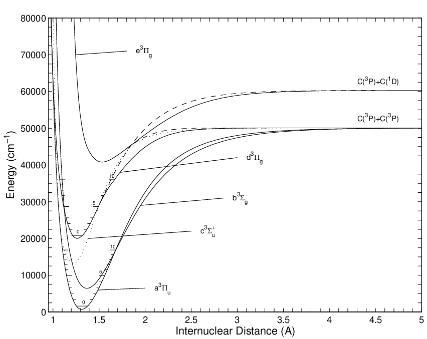
An analysis of the curve plots show that the perturbation of the d electronic state could be explained by the crossing of the b potential curve which occurs at =5. However for such cases, the perturbation would remain local, and higher vibrational levels of the d state would remain unperturbed, which is not the case. Therefore, the more probable cause for this perturbation could result from an avoided intersection between the d and e potential curves (see p. 295 in [28]), which alters the curve shape above the perturbation.
Dashed curve lines have been added to the plot to show the avoided intersection between the potential curves. The reconstruction of the unperturbed potential curve for the d electronic state has proceeded including solely the unperturbed levels =0–4 in the RKR calculation. The extrapolation of the potential curve by a Hulburth and Hirschfilder expression has taken into account a higher dissociation level [C(3P)+C(1D)]. The reconstruction of the e electronic state potential curve has proceeded identically, taking into account a lower dissociation level [C(3P)+C(3P)].
An experimental spectrum from the C2 Swan Bands v=0, obtained in the CORIA ICP torch for a low pressure CO2–N2–Ar plasma flow, has been simulated using the level constants proposed by Phillips, and their interpolation to equilibrium constants. The transition probabilities used in the calculation are issued from Cooper [45]. The comparison of the simulated spectra, using level and equilibrium spectroscopic constants to the experimental spectrum is presented in Fig. 6.

As it could be expected after the analysis of the fits presented in Fig. 4, it is verified that equilibrium constants, although fitted to very accurate level constants, fail to reproduce exactly the experimental spectrum. This is particularly apparent for the 1–1 bandhead at 5120 , which is not very well reproduced unlike the spectrum issued from level spectroscopic constants. Therefore, whenever vibrational perturbations are present for any of the states of the radiative transition, it is likely that the explicit insertion of level spectroscopic constants in simulation codes will be a required feature for a sufficiently accurate simulation.
3.2.3 The N First Negative System
A final example can be presented for a spectrum affected by rotational perturbations of it’s internal states (intersection of potential curves for ). For this case, there is a shift of the nearby levels populations following a mathematical expression of the type (see p. 283 in [28]). The more accurate but more complex method for accounting for the presence of such perturbations consists in solving the perturbative hamiltonian for the system [6]. However, in our case, it was chosen to resort to the usual Klein–Dunham coefficients for the calculation of the level energies, with the addition of a term in the form of
| (22) |
The upper electronic state B of the N First Negative System is known to be perturbed by the A electronic state. The influence of the shifts of levels energies on the observed spectrum are quickly appreciable, which makes this radiative system a good candidate for the illustration of the importance of perturbations modelling in spectral simulations. Such perturbations have been extensively studied in [47, 46], and the values for and (position and intensity of the perturbation) for the perturbations resulting from the above described interaction are reported in the references therein.
Emission from the N First Negative System system has been measured in the SR5 facility for a low pressure air plasma. The apparatus function of the measurement system has been set at a FWHM of 0.3 , which allows fully resolving the rotational lines of the spectrum. Spectral simulations have then been carried for this molecular system, firstly excluding, and lately taking into account the influence of the perturbations in the spectral model. Level spectroscopic constants provided by Michaud [47] and transition probabilities provided by Laux [48] have been taken into account for the calculations. The obtained results and a comparison with the experimental spectrum are presented in Fig. 7.

The analysis of the simulated spectra allows detecting large discrepancies due to the presence of perturbations. Namely, the structure of the 0–0 vibrational band is completely altered by the perturbations of the upper levels energies. The effects of the perturbations in the simulated spectrum are very apparent near 3900 . It can be verified that the simplified model used for including the effects of perturbations in the level energies allows obtaining a very close match to the experimental spectrum. This is no longer the case for the unperturbed spectrum, which fails to reproduce correctly the experimental spectrum, although accurate level spectroscopic constants are used in the calculation.
4 Conclusion
The methods and issues regarding line-by-line spectral calculations have been discussed in this paper. Accurate methods for calculating the main parameters of bound radiation such as line positions, intensities, and shapes, have been presented for diatomic rovibronic transitions, and linear polyatomic rovibratinal transitions.
Moreover, as line-by-line molecular simulations lead to the calculation of spectrums composed from a very large number of lines, with arising issues regarding computation times and memory limitations, strategies leading to a reduction in the number of calculated lines, with minor accuracy losses, have been presented.
A more complete discussion on the different methods available for the calculation of line positions has also been carried. Additionally to the necessity of selecting the most adapted method for the calculation of line positions, the importance of selecting the most accurate and adapted spectral dataset has been highlighted. It has been showed that coping with the specific issues of the simulation of unperturbed but also perturbed spectra may allow reaching simulated spectra that matches very accurately experimentally determined spectra. Moreover, achieving such accuracies in spectral simulations also results in a very suitable method for determining vibrational and rotational temperatures and to a good level of accuracy. The methods which were applied to the simulation of the presented experimental spectra have allowed determining the vibrational and rotational temperatures to an accuracy of 100 . Even when a Boltzmann equilibrium is not achieved for such levels, such methods can be successfully applied to the determination of the levels population distributions [53].
Acknowledgements
The author would like to acknowledge P. Boubert for providing the experimental spectrum of the C2 Swan Bands presented in this paper.
Appendix
Appendix A Multiplet Level Energies
All the expressions below are written in wavenumber units (\reciprocal).
Doublet Levels
The general expression for the doublet energy levels is given by [28]:
| (23c) | ||||
| (23f) | ||||
For states, a simpler expression of the levels energies is used [28]:
| (24a) | ||||
| (24b) | ||||
Triplet Levels
The more accurate expressions for states energy levels given by [50] form the formulae of [51] with a typographical correction from [5] are preferred to the ones found in [28]:
| (25a) | ||||
| (25d) | ||||
| (25e) | ||||
states energy levels are given by [52]:
| (26c) | ||||
| (26d) | ||||
| (26g) | ||||
with
Appendix B Coalesced, Weak and Strong Branches for Doublet and Triplet Transitions
Expressions for parallel transitions for Hünd case are taken from [17], expressions for parallel transitions for Hünd case are taken from [20], expressions for perpendicular and transitions for the intermediary case between Hünd cases and were taken from [18] and [16] respectively. Expressions for parallel and transitions for the intermediary case between Hünd cases and were taken from [19].
Weak Rotational Branches
For multiplet parallel transitions (), all the satellite rotational branches have weak strengths. For multiplet perpendicular transitions () the weak rotational branches are listed in Tab. 2
List of Coalesced Branches for Transitions Without Spin-Splitting Effects for the State
The coalesced rotational branches for multiplet transitions with a neglected spin-splitting of the state are listed in Tab. 3.
References
- [1] Laux C. O., Gessman R. J., Kruger C. H., Roux F., Michaud F., and Davis S. P., ”Rotational Temperature Measurements in Air and Nitrogen Plasmas Using the First Negative System of N”, J. Quant. Spectrosc. Radiat. Transfer, Vol. 68, pp. 473–482 (2001).
- [2] Laux C. O., Spence T. G., Kruger C. H., and Zare R. N., ”Optical Diagnostics of Atmospheric Pressure Air Plasmas”, Plasma Sources Sci. Technol., Vol. 12, pp. 125–138 (2003).
- [3] Park C., ”Stagnation-Point Radiation for Apollo 4”, Journal of Thermophysics and Heat Transfer, Vol. 18, No. 3, pp. 349–357 (2004).
- [4] Zare R. N., Schemeltekopf A. L., Harrop W. J. and Albritton D. L., ”A Direct Approach for the Reduction of Diatomic Spectra to Molecular Constants for the Construction of RKR Potentials”, Journal of Molecular Spectroscopy, No. 46, pp. 37–66 (1973).
- [5] Laux C. O., ”Optical Diagnostics and Radiative Emission of Air Plasmas”, Ph. D. Thesis, Stanford University, HTGL Report No. T-288 (1993).
- [6] Lefebvre-Brion H., and Field R. W., ”Perturbations in the Spectra of Diatomic Molecules”, Academic Press, Inc - London (1986).
- [7] Giordano D., Capitelli M., and Colonna G., ”Tables of Internal Partition Functions and Thermodynamic Properties of High-Temperature Air Species From 50 K to 100000 K”, ESA STR–237, ESA Publications Office (1994).
- [8] Capitelli M., Ferreira C. M., Gordiets B. F., and Osipov A. I., ”Plasma Kinetics in Atmospheric Gases”, Springer Series on Atomic, Optical, and Plasma Physics, Vol. 31 (2000).
- [9] Chernyi G. G., Losev S. A., Macheret S. O., and Potapkin B. V., ”Physical and Chemical Processes in Gas Dynamics: Cross Sections and Rate Constants, Vol. 1, AIAA Progress in Astronautics and Aeronautics, Vol. 196 (2002).
- [10] Sarrete J.–P., Gomes A.–M., Bacri J., Laux C. O., and Kruger C. H., ”Collisional-Radiative Modelling of Quasi-Thermal Air Plasmas With Electronic Temperatures Between 2000 and 13.000 K I. K”, J. Quant. Spectrosc. Radiat. Transfer, Vol. 53, No. 2, pp. 125–141 (1995).
- [11] Guerra V., Sá P. A., and Loureiro J., ”Kinetic Modelling of Low-Pressure Nitrogen Dischrges and Post-Discharges”, Eur. Phys. J. Appl. Phys., Vol. 28, pp. 125–152, 2004.
- [12] Corse G., Cacciatore M., and Capitelli M., ”Nonequilibrium Dissociation and Ionisation of Nitrogen in Electrical Discharges”, Chemical Physics, Vol. 66, pp. 141–151 (1982).
- [13] Capitelli M., Armenise I., and Gorse C., ”State-to-State Approach in the Kinetics of Air Components Under Re-Entry Conditions”, Journal of Thermophysics and Heat Transfer, Vol. 11, No. 4, pp. 570–578 (1997).
- [14] Armenise I., Capitelli M., Kustova E., and Nagnibeda E., ”The Influence of Nonequilibrium Kinetics on the Heat Transfer and Diffusion near Reentering Body”, Journal of Thermophysics and Heat Transfer, Vol. 13, No. 2, pp. 210–218 (1999).
- [15] Whiting E. E., ”Recommended Conventions for Defining Transition Moments and Intensity Factors in Diatomic Molecular Spectra”, Journal of Molecular Spectroscopy, Vol. 80, pp. 249–256 (1980).
- [16] Budò, A., ”Intensitätsformeln für die Triplettbanden”, Mitteilung aus dem Physikalischen Institut der Königl.-Ungarischen Universität für Technische und Wirtschaftwissenschaften, pp. 579–587 (1937).
- [17] Schadee A., ”The Formation of Molecular Lines in the Solar Spectrum”, Bull. Astron. Inst. Neth., Vol. 17, No. 5, pp. 311–357 (1964).
- [18] Arnold J. O., Whiting E. E., and Lyle, G. C., ”Line by Line Calculation of Spectra From Diatomic Molecules and Atoms Assuming a Voigt Line Profile”, J. Quant. Spectrosc. Radiat. Transfer, Vol. 9, pp. 775–798 (1969).
- [19] Kovacs I., ”Rotational Structure in the Spectra of Diatomic Molecules”, Adam Hilger Ltd. (1969).
- [20] Tatum J. B., and Watson J. K. G., ”Rotational Line Strengths in Transitions With Intermediate Coupling”, Canadian Journal of Physics, Vol. 49, pp. 2693–2703 (1971).
- [21] Cramer C. J., ”Essentials of Computational Chemistry: Theories and Models”, John Wiley & Sons (2004).
- [22] Rydberg R., ”Graphische Darstellung Einiger Bandenspektroskopischer Ergebnisse”, Zeitschrift für Physik, Vol. 73, pp. 376–385 (1931).
- [23] Klein O., ”Zur Berechnung von Potentialkurven für Zweiatomige Moleküle mit Hilfe von Spektraltermen”, Zeitschrift für Physik, Vol. 76, pp. 226–235 (1932).
- [24] Rees A. L., ”The Calculation of the Potential Energy Curves From Band–Spectroscopy Data”, Proceedings of the Physical Society, Vol. A59, pp. 998–1008 (1947).
- [25] Hulburt H. M. and Hirschfelder J. O., ”Potential Energy Functions for Diatomic Molecules”, Journal of Chemical Physics, Vol. 9, pp. 61–69 (1941).
- [26] Lino da Silva M., ”Simulation des Propriétés Radiatives du Plasma Entourant un Véhicule Traversant une Atmosphère Planétaire à Vitesse Hypersonique: Application à la planète Mars”, PhD Thesis (in French), Université. Orléans (2004).
- [27] Scutaru D., ”Etudes Théorique et Expérimentale de l’Absorption Infrarouge par CO2 à Haute Température. Application à des Modèles de Rayonnement des Gaz”, Ph.D. Thesis (in French), Laboratoire d’Energétique Moléculaire et Macroscopique, Combustion (E.M2.C), Ecole Centrale de Paris, France (1994).
- [28] Herzberg G., ”Spectra of Diatomic Molecules”, Second Edition, AD. Van Nostrand Company Inc. (1965).
- [29] Taine J., ”A Line-by-Line Calculation of Low-Resolution Radiative Properties of CO2–CO Transparent Nonisothermal Gases Mixtures up to 3000 K”, J. Quant. Spectrosc. Radiat. Transfer, Vol. 30, No. 4, pp. 371–379 (1983).
- [30] Gamache R. R., and Rothman L. S., ”Extension of the HITRAN Database to Non-LTE Applications”, J. Quant. Spectrosc. Radiat. Transfer., Vol. 48, No. 5/6, pp. 519–525 (1992).
- [31] Rothman L. S., Hawkins R. L., Wattson R. B., and Gamache R. R., ”Energy Levels, Intensities, and Linewidths of Atmospheric Carbon Dioxide Bands”, J. Quant. Spectrosc. Radiat. Transfer, Vol. 48, No. 5/6, pp. 537–566 (1992).
- [32] Jefferies J. T., ”Spectral Line Formation” Blaisdell Company, First Edition (1968).
- [33] Olivero J. J., and Longbothum R. L., ”Empirical fits to the Voight Line Width: A Brief Review”, J. Quant. Spectrosc. Radiat. Transfer, Vol. 17, pp. 233–236 (1977).
- [34] Schreier F., ”Voigt and Complex Error Function: A Comparison of Computational Methods”, J. Quant. Spectrosc. Radiat. Transfer, Vol. 48, No. 5/6, pp. 743–762 (1992).
- [35] Prasad C. V. V., and Bernath P. F., ”Fourier Transform Jet-Emission Spectroscopy of the Transition of CN”, Journal of Molecular Spectroscopy, No. 156, pp. 327–340 (1992).
- [36] Lago V., Lebéhot A., Dudeck M., Pellerin S., Renault T., and Echegut P., ”Entry Conditions in Planetary Atmospheres: Emission Spectroscopy of Molecular Plasma Arcjets”, Journal of Thermophysics and Heat Transfer, Vol. 15, No. 2, pp. 168–175 (2001).
- [37] Thebault-Leborgne L., ”Analyse Expérimentale d’un Plasma d’Argon Supersonique Turbulent Basse Pression”, Ph. D. Thesis (in French), Université de Rouen (1998).
- [38] Lino da Silva M., Lago V., Bedjanian E., Lebéhot A., Mazouffre S., Dudeck M., Szymanski Z., Peradzynski Z., Boubert P., and Chickhaoui A., ”Modelling of the Radiative Emission of a Plasma Surrounding an Atmospherical Probe for Mars Exploration”, High Temperature Material Processes, Vol. 7, No. 1, pp. 115–125 (2003).
- [39] Huber K. P., and Herzberg G., ”Molecular Spectra and Molecular Structure – IV. Constants of Diatomic Molecules”, Van Nostrand Reinhold Company (1979).
- [40] Park C., ”Nonequilibrium Air Radiation (NEQAIR) Program: User’s Manual”, NASA TM–86707, NASA Ames Research Center, Moffet Field, CA 94035 (1985).
- [41] Cerny D., Bacis R., Guelachvili G., and Roux F., ”Extensive Analysis of the Red System of the CN Molecule With a High Resolution Fourier Spectrometer”, Journal of Molecular Spectroscopy, Vol. 73, pp. 154–167 (1978).
- [42] Ito H., Ozaki Y., Suzuki K., Kondow T., and Kuchitsu K., ”Analysis of the Perturbations in the CN() Main Band System”, Journal of Molecular Spectroscopy, Vol. 127, pp. 283–303 (1988).
- [43] Knowles P. J., Werner H.-J., Hay J., and Cartwright D. C., ”The Red and Violet Systems of the CN Radical: Accurate Multireference Configuration Interaction Calculations of The Radiative Transition Probabilities”, J. Chem. Phys., Vol. 89, No. 12, pp. 7334–7343 (1988).
- [44] Phillips J. G., ”Perturbations in the Swan System of the Molecule”, Journal of Molecular Spectroscopy, Vol. 28, pp. 233–242 (1968).
- [45] Cooper D. M., and Nicholls R. W., ”Transition Probability Data for Seven Band Systems of ”, Spectroscopy Letters, Vol. 9, No. 3, pp. 139-155 (1976).
- [46] Michaud F., Roux F., Davis S. P., and Nguyen A. D., ”High-Resolution Fourier Spectrometry of ”, Applied Optics, Vol. 35, No. 16, pp. 2867–2873 (1996).
- [47] Michaud F., Roux F., Davis S. P., Nguyen A. D., and Laux C. O., ”High-Resolution Fourier Spectrometry of the Ion”, Journal of Molecular Spectroscopy, Vol. 203, pp. 1–8 (2000).
- [48] Laux C. O., and Kruger C. H., ”Arrays of Radiative Transition Probabilities for the First and Second Positive, NO Beta and Gamma, First Negative, and Schumann-Runge Band Systems”, J. Quant. Spectrosc. Radiat. Transfer, Vol. 48, No. 1, pp. 9–24 (1992).
- [49] Ballik E. A. and Ramsay D. A., ”An Extension of the Phillips System of C2 and a Survey of C2 States”, Astrophysical Journal, Vol. 137, No. 1, pp. 84–101 (1963).
- [50] Nicolet M., Cieslik S., and Kennes R., ”Aeronomic Problems of Molecular Oxygen Photodissociation - V. Predissociation in the Schumann–Runge Bands of Oxygen”, Planet. Space Sci., Vol. 37, pp. 427–458 (1989).
- [51] Miller S. L., and Townes C. H., ”The Microwave Absorption Spectrum of (O and O16O17”, Phys. Rev., Vol. 90, pp. 537–543 (1953).
- [52] Budò A., ”Über die Triplett-Bandentermformel für den Allge Meinen Intermediären Fall und Anwendung Derselben auf die , Terme des -Moleküls”, Z. Physik, Vol. 96, pp. 219–229 (1935).
- [53] Lino da Silva M., Passarinho P., and Dudeck M., ”Strong Shock-Wave Interaction With an Expanding Plasma Flow: Influence on the CN Molecule Internal Modes”, 24th Int. Symposium Rarefied Gas Dynamics, Bari, Italy, 11–16 July 2004.