Minority Games with heterogeneous timescales

The above definition of the MG assumes implicitely that all the agents may change the strategy that they use ($s_{i}(t)$) at each time step. Variants of the game where all the agents update synchronously their $s_{i}(t)$ every $T$ time steps have been studied in the literature Garrahan et al. 2000; Heimel and Coolen 2001; andTobias Galla 2003; Challet et al. 2004, and are exactly solvable in the limit $T\to\infty$, in which case they are called batch games. This part of the paper separates the populations into two groups. Fast agents behave as usual, whereas slow agents update their strategies synchronously every $T$ time steps. This introduces a heterogeneity of time scales. I n essence, it is similar to giving a longer history memory in games where the state $\mu(t)$ is the binary encoding of the last $M$ winning choice, also known as games with real histories. Giving a larger $M$ to a set of agents is already found in the very first paper on the MG, and was analyzed further in Hui et al. 1999; Challet et al. 2000a. Such agents do surprisingly worse than their colleagues as long as the system is not deep into the symmetric phase, which is characterized by alternating winning sides; Metzler Metzler 2002 showed that agents with a larger $M$ need a large alternating probability in order to be able to profit from it. The case we study here is much simpler as it does not require real histories and is a priori more suitable to mathematical understanding. Unfortunately, since the exact analytical solution does not exist for games where all the agents update synchronously their strategies every $T$ time steps, we cannot solve the mixed case either and must resort to numerical simulations.

The relative composition of the population is tuned by a parameter $\phi$: if $N$ is the total number of agents, $\phi N$ of them are ordinary Minority Game agents, i.e., fast, whereas $(1-\phi)N$ update their strategy choice variable $s_{i}(t)$ every $T$ time steps, that is, their scores evolve following

	$\displaystyle y_{i}^{s}(t+1)$	$\displaystyle=$	$\displaystyle y_{i}^{s}(t)-\sum_{t^{\prime}=t-T+1}^{t}a_{i,s}^{\mu(t^{\prime})}A(t^{\prime})~~{\rm if}~t~{\rm MOD}~T=0$
	$\displaystyle y_{i}^{s}(t+1)$	$\displaystyle=$	$\displaystyle y_{i}^{s}(t)~~{\rm otherwise.}$		(2)

As usual, we shall focus on the predictability

$$H=\frac{1}{P}\sum_{\nu=1}^{P}\langle{A|\nu}\rangle^{2}$$

(3)

where $\langle{A|\nu}\rangle$ is the temporal average of $A$ conditional to $\mu(t)=\nu$. If $H>0$, knowing $\mu$ makes it possible to predict statistically the next outcome. $H$ measures the amount of information left by the agents in the game. The fluctuations $\sigma^{2}=\langle{A^{2}}\rangle$ play a special role as they quantify the quality of resource sharing achieved by the population, which is usually benchmarked against the fluctuations produced by random choice $\sigma^{2}/N=1$. It is easy to see indeed that the $\sigma^{2}$ is nothing else than the average total loss per time step of the population. Of particular interest in the case of competing populations are their respective average gains per time step.

Figure 1 reports the behaviour of $H$ and $\sigma^{2}$ as a function of $\alpha=P/N$, for a fixed $\phi$ and different values of $T$. In the predictable, asymmetric phase ($H>0$), the slow agents do not change the unique stationary state; as a result, $H$ does not depend on $T$, but $\sigma^{2}$ is slightly lowered as $T$ increases, because strategy switching occurs less often. On the other hand, in the unpredictable, symmetric phase ($H=0$), multiple stationary states exist as a result of broken ergodicity Challet et al. 2000b; Heimel and Coolen 2001, and any modification to the system will accordingly change the final values of $\sigma$. This is the case here: the introduction of a small amount of slow agents reduces the total amount of fluctuations because they damp the overreaction of the fast players without contributing too much to the global outcome $A$.

What is more surprising is the behaviour of $\sigma^{2}$ in the symmetric phase when one varies $\phi$, as shown in Fig. 2: at fixed $\alpha=0.2$, slow agents ($\phi=0$) produce larger fluctuations than fast ones ($\phi=1$); increasing the fraction of fast agents $\phi$ decreases the fluctuations which reaches a minimum below $1$, the random choice benchmark, and then increase again to reach the standard MG value, slightly above $1$. This means that the two groups live in symbiosis, and that there is a non-trivial optimal composition of the population. Other known examples of symbiosis in MGs include speculators and producers Challet et al. 2000a.

In such cases, it is natural to characterize the information ecology of the model (see Zhang 1999; Challet et al. 2000a), that is, who exploits who. To this end, Fig. (3) reports the average gain per time step of fast agents $\gamma_{f}$, which decreases monotonically as their concentration $\phi$ increases, but stays roughly constant as long as $\phi<0.4$. In this region, the slow agents provide information that the fast agents exploit. The losses of the latter are greatly reduced compared to $\phi=1$, but they seem not to be able to achieve positive gain on average. Similarly, when the slow agents are few ($\phi>0.8$), they profit from overreacting fast agents.

In the standard MG, all the $a_{i,s}^{\mu}$ are random variables, drawn completely independently from each other. Take an agent with two strategies; they will stipulate the same action a fraction $c=1/2$ of the $\mu$s on average. In other words, the standard-MG agents behave in the same way irrespectively on their strategy choice for half of the market states $\mu$.¹¹ 1 This is the origin of predictability in the MG Challet and Marsili 1999. MG with tunable $c$ where introduced in Ref. Challet et al. 2000a and also studied later in Refs Sherrington et al. 2002; andTobias Galla 2003. The parameter $c$ induces a reaction time scale $\sim 1/(1-c)$: the smaller $c$, the more adaptive an agent is; on the other end, people with $c=1$ are not adaptive: they inject predictability and are ideal candidates for exploitation. The latter were introduced as producers, that is, people who do not care much about timing in market, but use the market as a tool for exchanging goods Zhang 1999; producers ($c=1$) and speculators ($c<1$) live in symbiosis Challet et al. 2000a, that is, the gain of a given group increases then the other group is also present.

Here, we consider the case where the two groups $s$ and $f$ have $0\leq c_{g}<1$, $g=s,f$. The apparent similarity of this setup with the case previously studied Challet et al. 2000a is deceptive, as we shall see. The strategies are drawn according to

	$\displaystyle P_{f}(a^{\mu}_{i,1}=a^{\mu}_{i,2})$	$\displaystyle=$	$\displaystyle c_{f};$		(4)
	$\displaystyle P_{s}(a^{\mu}_{i,1}=a^{\mu}_{i,2})$	$\displaystyle=$	$\displaystyle c_{s}.$		(5)

When $c_{f}<c_{s}$, group $f$ is the fast one, and group $s$ is the slow one. The asymmetric phase of the model for an arbitrary number of groups is exactly solvable in the limit $N\to\infty$ with replica trick Mézard et al. 1987; Challet et al. 2000b; Challet et al. 2000a. The solution gives

$\displaystyle\frac{H}{N}=\frac{\phi c_{f}+(1-\phi)c_{s}+\phi(1-c_{f})Q_{f}+(1-\phi)(1-c_{s})Q_{s}}{(1+\phi\chi_{f}+(1-\phi)\chi_{s})^{2}}$

(7)

where $Q_{g}=\sum_{i\in{\cal N}_{g}}\langle{s_{i}(t)}\rangle^{2}$ ($g=f,s$); $\chi_{f}$ and $\chi_{s}$ are the integrated response functions Heimel and Coolen 2001. These four quantities all depend on two variables $\zeta_{f}$ and and $\zeta_{s}$ which are the solutions of two coupled non-linear equations (see appendix). Eq. (7) shows that in this case the stationary state of the asymmetric phase depends on the composition of the population, which is also true of the location of the critical point.

The respective gains of the two groups can also be computed exactly. Starting from the total losses

$\displaystyle\frac{\sigma^{2}}{N}=\frac{H}{N}+\phi(1-c_{f})(1-Q_{f})+(1-\phi)(1-c_{s})(1-Q_{s})$

(8)

and observing that if $\sigma^{2}_{\lambda}=\sum_{\mu=1}^{P}\langle{(A_{\rm fast}+\lambda A_{\rm slow})^{2}|\mu}\rangle/P$, the gains of the agents are nothing else than

	$\displaystyle\gamma_{s}$	$\displaystyle=$	$\displaystyle-\langle{A_{\rm slow}A}\rangle=-\frac{1}{2}\left.\frac{\partial\sigma^{2}_{\lambda}}{\partial\lambda}\right|_{\lambda=1}$		(9)
	$\displaystyle\gamma_{f}$	$\displaystyle=$	$\displaystyle-\sigma^{2}-\gamma_{s}.$		(10)

From the replica calculus, we find

$\displaystyle\frac{\gamma_{s}}{N_{s}}$

$\displaystyle=$

$\displaystyle\frac{H}{N}\chi_{s}-\frac{c_{s}+(1-c_{s})Q_{s}}{1+\phi\chi_{f}+(1-\phi)\chi_{s}}-(1-c_{s})(1-Q_{s});$

(11)

$\displaystyle\frac{\gamma_{f}}{N_{f}}$

$\displaystyle=$

$\displaystyle-\frac{1}{\phi}\frac{\sigma^{2}}{N}-\frac{1-\phi}{\phi}\frac{\gamma_{s}}{N_{s}}.$

(12)

The behaviour of the game is non trivial, which is already clear in Fig 4, where the fluctuations, or average losses of the players per time-step, are plotted agains $c_{s}$, showing a maximum. In this kind of plot, one should be careful to stay in the asymmetric phase, because the critical point $\alpha_{c}$ depends on $c_{s}$, $c_{f}$, and $\phi$. Taking $\alpha>1$ solves this problem since $\alpha_{c}\leq 1$. The minimum of $\sigma^{2}/N$ is surprising at first. Figure 5 gives a deeper understanding of this peculiar phenomenon by plotting the gains of the two groups. The minimum of the losses can be attributed entirely the slow agents only, who profit quite remarkably from the fast agents ($c_{f}=0$) unless they are very slow. This shows an competition between two effects: being slower means that one overreact less, in particular with respect to local fluctuations; inversely, being too slow makes it too difficult to react to being exploited. Interestingly, increasing $c_{s}$ increases monotonically the gains of group $f$.

The relative fraction of each type of agent is a crucial parameter, as illustrated by Fig 5, in particular when one group of agents has a large strategy correlation. In order to shed more light on the matter, we produced plots of the regions where one group has an advantage over the other. When $\phi=0.5$, Figure 6 contains four regions of interest. When $c_{g}<c^{*}\simeq 0.61$, group $g$ on average wins more than the other group $g^{\prime}$ as long as $c_{g}>c_{g}^{\prime}$, which means that as long as both groups have sufficiently low $c$s, the slower the better. On the other hand, when $c_{g}>c^{(}m)\simeq 0.98$, group $g^{\prime}$ always exploits group $g$. For intermediate values of $c_{g}$, the outcome depends on the precise value of both $c_{g}$ and $c_{g}^{\prime}$. While changing $\phi$ leaves unaffected the diagonal boundary, it has two remarkable effects: first it changes the non-linear boundary between the $\gamma_{f}<\gamma_{s}$ and $\gamma_{s}<\gamma_{s}$ regions by roughly rotating it clockwise. A new region also appears for $\alpha$ and $\phi$ small enough where the gain of group in relative sparseness is positive; it is however very small, and only appears when the largest group has a very large $c$. In this case, one needs to be few and react fast in order to be able to exploit very slow agents so much that one’s gain is positive.

Let us consider $G$ groups of respectively $\phi_{g}N$ agents, $g=1,\cdots,G$; all the agents belonging to group $g$ have $\Gamma_{g}$. Using the notation $\overline{f(x_{g})}=\sum_{g}\phi_{g}f(x_{g})$ for any function $f$ of variables $x_{g}$, the dynamical equation for $\Delta$ reads now

$$\Delta(t+1)=\Delta(t)-\overline{\tanh[\Gamma_{g}\Delta(t)]}+\eta(t)$$

(26)

where $\eta_{g}(t)$ are Gaussian noises with zero average and variance $\langle{\eta(t)\eta(t^{\prime})}\rangle=\delta_{t,t^{\prime}}\frac{(1-\overline{\tanh(\Gamma_{g}\Delta)^{2}}}{N}$. Linear stability shows that $\Delta^{(0)}$ is a stable fixed point as long as

$$\overline{\Gamma_{g}}<2.$$

(27)

When this point is unstable, it replaced by a period-two dynamics with stable point

$$\Delta^{(1)}=\frac{\overline{\tanh(\Gamma_{g}\Delta^{(1)})}}{2}$$

(28)

Going through the same procedure as before, one finds that $P(\Delta)$ is determined by

$$\frac{\textrm{d}P}{P}=\frac{-2N\overline{\tanh(\Gamma_{g}\Delta)}[1+\overline{\Gamma_{g}(1-\tanh(\Gamma_{g}\Delta)^{2}}]-2\overline{\Gamma_{g}\tanh(\Gamma_{g}\Delta)[1-\tanh(\Gamma_{g}\Delta)^{2}]}}{N\overline{\tanh(\Gamma_{g}\Delta)}^{2}+1-\overline{\tanh(\Gamma_{g}\Delta)^{2}}}$$

(29)

This cannot be integrated any more. The Gaussian approximation consists in keeping only the terms linear in $\Delta$ in this equation, and results in $\Delta$ being of average $0$ and variance $\langle{\Delta^{2}}\rangle=\frac{1}{2[N\overline{\Gamma_{g}}(1+\overline{\Gamma_{g}})-\overline{\Gamma_{g}^{2}}]}$ for small $\Gamma$.

The average gain per player of group $g$ at fixed $\Delta$ is equal to

$$\frac{\langle{\gamma_{g}|\Delta}\rangle}{N_{g}}=-\frac{\langle{A_{g}^{2}|\Delta}\rangle+\sum_{g^{\prime}\neq g}{\langle{A_{g}A_{g}^{\prime}|\Delta}\rangle}}{N_{g}}=-1-(N_{g}-1)\tanh(\Gamma_{g}\Delta)^{2}-\tanh(\Gamma_{g}\Delta)\sum_{g^{\prime}}N_{g}^{\prime}\tanh(\Gamma_{g}^{\prime}\Delta)$$

(30)

Assuming that the Gaussian approximation is valid, i.e. if all the $\Gamma_{g}$ are small,

$$\frac{\langle{\gamma_{g}}\rangle}{N_{g}}\simeq-1-\Gamma_{g}\langle{\Delta^{2}}\rangle\left[-\Gamma_{g}+N\overline{\Gamma_{g}}\right]\to-1-\frac{\Gamma_{g}}{2[1+\overline{\Gamma_{g}}]}$$

(31)

for infinite $N$. The gain of an agent of group $g$ can be compared to the average gain, which yieds

$$\langle{\gamma_{g}}\rangle-\overline{\langle{\gamma_{g}}\rangle}\to\frac{\overline{\Gamma_{g}}-\Gamma_{g}}{2(1+\overline{\Gamma_{g}})}.$$

(32)

In other words, the smaller $\Gamma_{g}$, the smaller the losses of that group. This is intuitive: at a given time, i.e. at a given $\Delta$, the fraction of players whose action is opposite to the sign of $\Delta$ is larger for smaller $\Gamma$.

Figure 8 compares $\langle{\gamma}\rangle$ from numerical simulations and from Eq (31). As before, the approximations made are valid for small $\Gamma$. This figure also indicates that the transition at $\Gamma^{*}$ is smooth.

Another way of having heterogeneous time scales is to differ in one’s score memory. Before studying groups, let us again characterise first the homogeneous case. For the sake of simplicity, we consider exponential moving averages. There are two ways of implementing them:

$$\Delta(t+1)=\Delta(t)(1-\lambda)-\frac{A(t)}{N}$$

(33)

and

$$\Delta^{\prime}(t+1)=\Delta^{\prime}(t)(1-\lambda)-\lambda\frac{A^{\prime}(t)}{N}$$

(34)

The length of score memory is $1/|\ln(1-\lambda)|\propto 1/\lambda$ for small $\lambda$. One can transform Eq (33) into (34) by setting $\Delta^{\prime}=\Delta\lambda$ and $\Gamma^{\prime}=\Gamma/\lambda$. The same stability analysis as above gives for a homogeneous population

$$\Gamma+\lambda<2$$

(35)

and

$$\lambda(\Gamma^{\prime}+1)<2$$

(36)

Increasing $\lambda$ at fixed $\Gamma$ and $\Gamma^{\prime}$ has therefore opposite effects for the two kinds of dynamics: a small $\lambda$ stabilises Eq (33) and destabilises Eq (34). Since there is a one-to-one correspondance between all the results of Eqs (33) and (34), we shall focus on Eq (33). The period-two fixed point for $\Gamma+\lambda>2$ is now determined by $\Delta^{(1)}=\frac{1}{2-\lambda}\tanh(\Gamma\Delta^{(1)})$. Assuming that $\Delta^{(0)}=0$ is stable, the same procedure as before yields

$$\frac{\textrm{d}P}{P}=-2N\frac{[\lambda\Delta+\tanh(\Gamma\Delta)](1+\lambda+\Gamma[1-\tanh(\Gamma\Delta)])+\Gamma\tanh(\Gamma\Delta)[1-\tanh(\Gamma\Delta)^{2}]}{N(\lambda\Delta+\tanh(\Gamma\Delta))^{2}+1-\tanh(\Gamma\Delta)^{2}}$$

(37)

In the Gaussian approximation, one finds

$$\langle{\Delta^{2}}\rangle=\frac{1}{2[(\Gamma+\lambda)(1+\lambda+\Gamma)N-\Gamma^{2}]}.$$

(38)

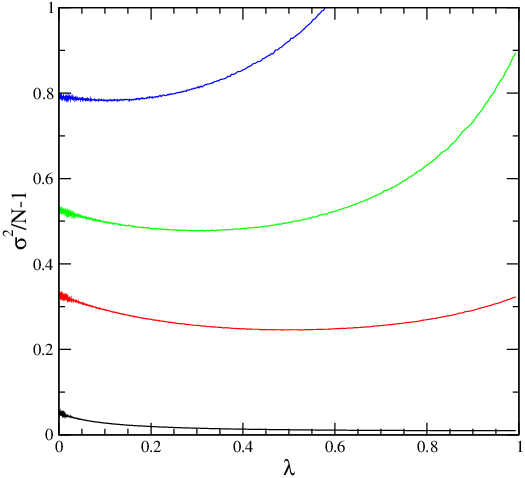
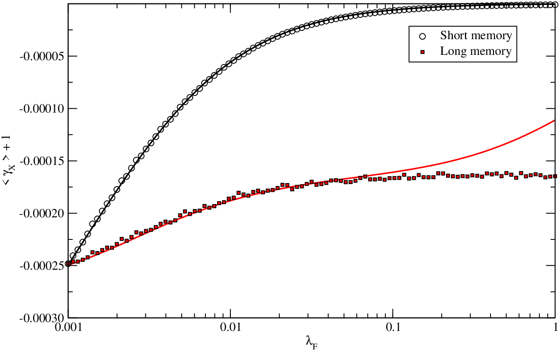
As consequence, for small $\Gamma$, $\lambda>0$ decreases the fluctuations. The Fokker-Planck equation holds if $\lambda+\Gamma<1$; otherwise, the change of sign of $\Delta$ at each time step (neglecting the noise) causes more fluctuations. Therefore, $\sigma^{2}/N$ has a minimum at $\lambda+\Gamma=1$ when $\lambda$ increases, as illustrated by Fig 9. The Gaussian approximation is very good for small $\Gamma$ and $\lambda$.

Generalising these results to groups of agents is more complicated than for heterogeneous $\Gamma$ because of the role of $\lambda$ in Eq. (33): each group $g$ with a given $\lambda_{g}$ has its own $\Delta_{g}$

$$\Delta_{g}(t+1)=\Delta_{g}(t)(1-\lambda_{g})-\overline{\tanh(\Gamma\Delta_{g^{\prime}})}+\eta(t)=f_{g}(\{\Delta_{g^{\prime}}\})+\eta(t)$$

(39)

where $\langle{\eta(t)\eta(t^{\prime})}\rangle=\delta_{t,t^{\prime}}(1-\overline{\tanh(\Gamma\Delta_{g^{\prime}})^{2}})/N$. For infinite $N$, the linear stability conditions of the fixed point $\Delta_{g}=0$ for all $g$ are $\sum_{g^{\prime}}|\partial f_{g}/\partial\Delta_{g^{\prime}}|<1$, that is,

$$|1-\lambda_{g}-\phi_{g}\Gamma_{g}|+\sum_{g^{\prime}\neq g}\phi_{g^{\prime}}\tanh(\Gamma_{g^{\prime}}\Delta_{g^{\prime}})<1\\$$

(40)

for all $g$. When $\lambda_{g}+\phi_{g}\Gamma_{g}<1$, i.e. both $\lambda_{g}$ and $\Gamma$ are small, the stability condition is $\overline{\Gamma_{g^{\prime}}}<\lambda_{g}+2\phi_{g}\Gamma_{g}$; for instance if $\Gamma_{g}=\Gamma$ for all $g$, and $\phi_{g}=1/G$, then the condition is $\Gamma(1-2/G)<\lambda_{g}$. The other case is obtained when $\Gamma_{g}\sim 1/\phi_{g}$ and gives $\lambda_{g}+\overline{\Gamma_{g^{\prime}}}<2$, which is the same as before. Interestingly, some unstable $\Delta^{(0)}_{g}$ can coexist with stable ones, for instance when $\Gamma_{g}=\Gamma=2-\epsilon$, $0<\epsilon\ll 1$, $\phi=1/G$ and $\lambda_{g}=2\epsilon g/G$, where the dynamics of $\Delta_{g}$ is stable for $g<G/2$ and unstable otherwise. This is clearly a source of losses for fast-forgetting players. Going back to the average gain per player per time step, ones indeed that the gain of group $g$ is intimately related to the variance of $\Delta_{g}$. The multivariate Fokker-Planck equation reads

$$\frac{\partial P(\Delta,t)}{\partial t}=\sum_{g}\frac{\partial}{\partial\Delta_{g}}\left[\left([\lambda_{g}\Delta_{g}+\overline{\tanh(\Gamma\Delta_{g^{\prime}})}]P\right)+\frac{1}{2}\sum_{g,g^{\prime}}\frac{\partial}{\partial\Delta_{g^{\prime}}}(D_{g,g^{\prime}}P)\right]$$

(41)

with

$$D_{g,g^{\prime}}=\frac{1-\overline{\tanh(\Gamma_{g^{\prime\prime}}\Delta_{g^{\prime\prime}})^{2}}}{N}+(\lambda_{g}\Delta_{g}+\overline{\tanh(\Gamma_{g^{\prime\prime}}\Delta_{g^{\prime\prime}})})(\lambda_{g^{\prime}}\Delta_{g^{\prime}}+\overline{\tanh(\Gamma_{g^{\prime\prime}}\Delta_{g^{\prime\prime}})})$$

(42)

Solving a linearised version of Eq (41) is done following standard procedure van Kampen 1992 and gives a multivariate Gaussian solution. For $G=2$, we have the resulting equations.

$\displaystyle P(\Delta_{f},\Delta_{s})$

$\displaystyle=$

$\displaystyle\frac{1}{2\pi\sigma_{f}\sigma_{s}\sqrt{1-\rho^{2}}}\exp\left[-\frac{1}{2(1-\rho^{2})}\left(\frac{\Delta_{f}^{2}}{\sigma_{f}^{2}}-\frac{2\rho\Delta_{f}\Delta_{s}}{\sigma_{f}\sigma_{s}}+\frac{\Delta_{s}^{2}}{\sigma_{s}^{2}}\right)\right]$

(43)

The expressions for $\sigma_{f}$, $\sigma_{s}$ and $\rho$ are too long to be reported here ³³ 3 We provide however a Mathematica file at www.maths.ox.ac.uk/ challet. Reusing Eq (30) the respective average gain is

	$\displaystyle\langle{\gamma_{f}}\rangle$	$\displaystyle\simeq$	$\displaystyle-1-\Gamma^{2}\left(\langle{\Delta_{f}^{2}}\rangle(N_{f}-1)+N_{s}\langle{\Delta_{f}\Delta_{s}}\rangle\right)$		(44)
		$\displaystyle=$	$\displaystyle-1-\Gamma_{f}^{2}\sigma_{f}^{2}(N_{f}-1)-\Gamma_{f}\Gamma_{s}N_{s}\rho\sigma_{f}\sigma_{s}]$

Figure 10 plots the gains of the two groups and clearly shows that all other things beeing equal, having a shorter memory is an advantage. Indeed, when $\Gamma_{f}=\Gamma_{s}=\Gamma$ and $\phi_{f}=\phi_{s}=1/2$, as in Fig. (10), Eq (44) leads to

	$\displaystyle\langle{\gamma_{f}}\rangle-\langle{\gamma_{s}}\rangle$	$\displaystyle\simeq$	$\displaystyle\frac{8\Gamma^{2}(\lambda_{f}-\lambda_{s})(1+\Gamma+\lambda_{f}+\lambda_{s})[\lambda_{f}(1+\lambda_{f}+\frac{\Gamma}{2})+\lambda_{s}(1+\lambda_{s}+\frac{\Gamma}{2})+\lambda_{f}\lambda_{s}]}{[2\lambda_{f}\lambda_{s}+\Gamma(\lambda_{f}+\lambda_{s})][4\Gamma^{2}+2(2+2\lambda_{f}+\lambda_{s})(2+\lambda_{f}+2\lambda_{s})+3\Gamma(4+3\lambda_{f}+3\lambda_{s})]}$		(45)
			$\displaystyle\times\frac{1}{2\Gamma^{2}+\Gamma(2+3\lambda_{f}+3\lambda_{s})+2(\lambda_{f}+\lambda_{f}^{2}+\lambda_{s}+\lambda_{s}^{2}+\lambda_{f}\lambda_{s})}$

which is of course positive when $\lambda_{f}>\lambda_{s}$. The above sections suggest that such advantage is menaced by increasing $\Gamma_{f}$. Interestingly, increasing $\phi_{f}$ increases the gains of both groups, as the fast agents suffer less from the fluctuations caused by their slow colleagues. In the unstable region, the effect is the opposite, that is, fast forgetting agents fail to smooth out sufficiently slowly large fluctuations, and suffer from larger losses than slower agents. We performed similar numerical simulations for $P>1$ and $\Gamma=\infty$ (standard MG), and found out similar results: faster agents end up earning less in both phases (we could not find an opposite result), which can be interpreted by their tendency to switch more often between their strategies.

References

- Olsen et al. (1992) R. Olsen et al., Tech. Rep. RBO.1992-09-07, Olsen & Associates (1992).
- Borland and Bouchaud (2005) L. Borland and J.-P. Bouchaud (2005), preprint physics/0507073.
- and (2003) G. Z. and, Quant. Fin. 3, 320 (2003).
- Marsili and Piai (2002) M. Marsili and M. Piai, Physica A 310, 234 (2002), cond-mat/0202479.
- Martino (2003) A. D. Martino, Eur. Phys. J. 35, 143 (2003).
- Arthur (1994) B. W. Arthur, Am. Econ. Rev. 84, 406 (1994).
- Heimel and Coolen (2001) J. A. F. Heimel and A. A. C. Coolen, Phys. Rev. E 63, 056121 (2001), cond-mat/0012045.
- andTobias Galla (2003) D. S. andTobias Galla, Physica A 324, 25 (2003).
- Garrahan et al. (2000) J. P. Garrahan, E. Moro, and D. Sherrington, Phys. Rev. E 62, R9 (2000), cond-mat/0004277.
- Challet et al. (2004) D. Challet, A. D. Martino, M. Marsili, and I. Peréz-Castillo (2004), cond-mat/0407595.
- Challet et al. (2000a) D. Challet, M. Marsili, and Y.-C. Zhang, Physica A 276, 284 (2000a), cond-mat/9909265.
- Hui et al. (1999) N. J. P. Hui, D. Zheng, and M. Hart, J. Phys. A: Math. Gen. 32, L427 (1999).
- Metzler (2002) R. Metzler, J. Phys. A: Math. Gen. 35, 721 (2002).
- Challet et al. (2000b) D. Challet, M. Marsili, and R. Zecchina, Phys. Rev. Lett. 84, 1824 (2000b), cond-mat/9904392.
- Zhang (1999) Y.-C. Zhang, Physica A 269, 30 (1999).
- Sherrington et al. (2002) D. Sherrington, E. Moro, and J. P. Garrahan, Physica A 311, 527 (2002), cond-mat/0010455.
- Mézard et al. (1987) M. Mézard, G. Parisi, and M. A. Virasoro, Spin glass theory and beyond (World Scientific, 1987).
- Marsili and Challet (2001) M. Marsili and D. Challet, Phys. Rev. E 64, 056138 (2001), cond-mat/0102257.
- Marsili (2001) M. Marsili, Physica A 299, 93 (2001).
- van Kampen (1992) N. G. van Kampen, Stochastic processes in Physics and Chemistry (North-Holland, 1992), chap. 8, p. 211.
- Challet and Marsili (1999) D. Challet and M. Marsili, Phys Rev. E 60, R6271 (1999), cond-mat/9904392.
- Savit et al. (1999) R. Savit, R. Manuca, and R. Riolo, Phys. Rev. Lett. 82, 2203 (1999).
- Andersen and Sornette (2003) J. V. Andersen and D. Sornette, Eur. Phys. J. B 31, 141 (2003), cond-mat/0205423.
- Giardina and Bouchaud (2002) I. Giardina and J.-P. Bouchaud (2002).
Appendix A Replica calculus
The calculus parallels mostly the established procedure Challet et al. 2000b; Challet et al. 2000a: the dynamics minimizes Marsili and Challet 2001 that is akin to an energy. The stationary state of the system corresponds therefore to the ground state of . After some algebraic manipulations it is possible to find relations that link the quantities that we have introduced The predictability is given by