Simulation of a fine grained GEM used in the PixiE Experiment
PixiE Internal Reporthttp://glastserver.pi.infn.it/pixie/pixie.html

M. Del Prete Affiliation: INFN and University, Pisa

15 May 2005

Introduction

We have simulated the performances of a GEM with a large density of multiplication holes. The elementary cell is an equilateral triangle whose side is 90 $\mu m$ . We shall assume that this pattern extends in the (x,y) plane. At each vertex of the equilateral triangle there is a GEM hole with an external radius of 30 $\mu m$ and an internal radius of 20 $\mu m$ . The reference frame used in this study has the origin of axis in the center of the GEM hole with the z axis pointing to the drift plane. The geometry of the GEM is shown in figure 1.

Refer to caption — Figure 1: A section of the hole of GEM. The red circles indicate the starting points of electrons.

In this short note we will describe the simulation of the GEM and, in particular we will study the gain and diffusion of the charge for different gas mixtures. This study has been performed to finalize the design of the PixiE Imager Detector.

We have started the simulation by generating single electrons in different positions in the (x,y) plane at fixed z-coordinate. This is the most elementary element through which we can simulate tracks and the imaging performance of the detector. The process has been followed through multiplication in the large fields of the GEM and diffusion of produced electrons reaching the readout plane. Due to the cylindrical symmetry of the GEM the first quadrant ( $x>0,y>0$ , see figure 1) has been selected to produce the coordinate ( $r$ , $\phi$ ) of the starting electrons at the quota of $40\;\mu m$ (approximately $15\;\mu m$ over the top GEM):

r=10\cdot{n}\;\mu m\quad(n\;=1,\;2,\;3)\qquad\phi=\frac{\pi}{2}\cdot{\frac{(k-1)}{3}}\quad(k\;=\;1,\;2,\;3,\;4)

Where $\phi$ is the azimuthal angle.

At each point we have generated 25 events. The study has been performed for the following gas mixtures:

•

100% $CO_{2}$ atm 0.5 ed 1 atm.
•

20%Ar/80%DME, 50%Ar/50%DME, 80%Ar/20%DME ad 1 atm.

Gain Study

We have defined as absolute gain the number of electrons which reach the quota $z\;=\;-40\mu m$ (below the plane the GEM, approximately $15\mu m$ below the bottom GEM plane). At this quota most of the multiplication processes at the GEM hole are done.

However not all these electrons drift to the readout plane, some recombine and many stick to the lower GEM plane (re-attachment). For this reason we have defined also an effective gain as the number of electrons which arrive at the quota $z\;=\;-200\mu m$ . The electrons reaching this quota are considered to be collected by the read out plane.

It’s customary to describe the gain with a Polya:

P_{n}=\frac{1}{b\cdot\overline{n}}\cdot\frac{1}{\Gamma\left(\frac{1}{b}\right)}\cdot\left(\frac{n}{b\cdot\overline{n}}\right)^{\left(1/b\right)-1}\cdot e^{-n/b\cdot\overline{n}}

Where $b$ is an adjustable parameter and $\overline{n}$ is the average gain. We have used this formula and fit the data with the function:

F(n;p_{0},p_{1},p_{2})=p_{2}\cdot n^{p_{0}-1}\cdot e^{-n/p_{1}}

where $p_{2}$ is a normalization factor and the gain is the Polya mean, $G\;=\;p_{0}\;\cdot\;p_{1}$ .

The gain distribution is different for different mixtures of gases. In particular the absolute gain distribution is often wide with long tails and a description with a single Polya is not always satisfactory. Hence, we have described the distribution with the sum of two Polya, of which the first one fits most of events and the second one accounts for the long tails. An example is shown in figure 2. We have taken as the average gain of the GEM the mean of the first Polya.

Sometimes the distribution shows two clear maxima and a two Polya fit is satisfactory. In this case the mean of the two Polya is the average gain of the GEM under analysis. Results are shown in the figure 3, 4 for a collecting field $E_{t}\;=\;4KV/cm$ and two gas mixtures and in the table 1 for a collecting field of $E_{t}\;=\;5KV/cm$ .

$\Delta V_{GEM}=560\;V\quad E_{Trasf}=5KV/cm$	$p=0.5atm$	$p=1atm$
$Gain_{eff}$	830 $\pm$ 100	70 $\pm$ 10
$Gain_{ass}$	7420 $\pm$ 400	2400 $\pm$ 900

Table 1: Average of effective and absolute gain of 100%

CO_{2}

at 0.5 and 1 atm and for

\Delta V_{GEM}

560V

and collection field of

5KV/cm

The GEM gain increases with the voltage different GEM according to an exponential curve.

Diffusion Study

The study of the diffusion of the charge in the collecting region of the detector is important for two different issues.

Firstly to establish if the GEM keeps memory of the starting point of the electrons, both in azimuth and radius (with respect to the center of the hole where the avalanche occurs) with a better resolution than the granularity of GEM’s hole.

For this, we have studied the position of the barycentre of charge arrived on readout plane (barycentre of the avalanche) as a function of the position of the starting point.

The second point is the RMS of Gaussian distribution of charge in the collection gap which is related with the spatial resolution of the detector.

The average position of the collected charge indicates where the multiplication occurs at the GEM hole.

We have considered

\Delta R\;=\;R_{fin}\;-\;R_{in}

where $R_{in}\;=\;r$ and $R_{fin}$ is the radius of the average charge at the quota $z\;=\;-200\mu m$ . First of all we have studied the dependence of $\Delta R$ on $R_{in}$

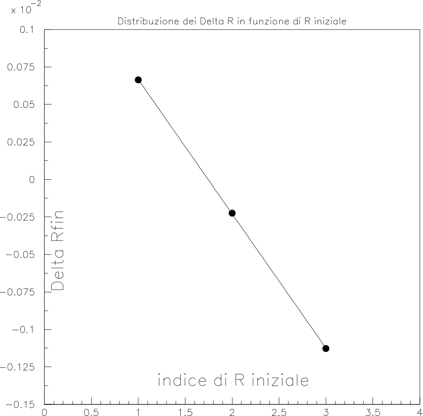
The figure 5 shows an example of such a dependence. $\Delta R$ is a linear function of $R_{in}$ and a parameterization: $\Delta R\;=P_{2}R_{in}\;+\;P_{1}$ with $P_{2}\approx-1$ and $P_{1}\approx 20\mu m$ is a good fit for all simulations (figure 6). For a ideal GEM $\Delta R=0$ in fact this means that the position (in radius) of the multiplied charge is the same as the initial electron (the GEM does not disturb the image). The results of the fit shows instead that the average collected charge position is independent of the starting position ( $P_{2}\approx-1$ ) and that the multiplication occurs at the radius $r\approx 20-30\mu m$ (the lower external radius).

The last step is the study of the dispersion of the avalanche’s charge after it drifted to the collection electrodes.

We have averaged the RMS of the events produced at each point and verified that its value is independent of the position of primary electron. Hence we have averaged the RMS of all events at all points, to improve the statistics and studied its dependence on the GEM voltage. Since, again, we have found no dependence, we have average on all events for a defined gas composition.

The results for 100% $CO_{2}$ gas at $0.5\;atm$ are:

•

$RMS_{p}\;=\;12.5\;\mu m$
•

$RMS_{sp}\;=\;17.67\;\mu m$

The results for Argon and Neon mixtures are shown in figure 7, the RMS decreases mildly with increasing percentage of Argon and Neon.

Acknowledgments

I would like ti thank G.Spandre for the help and continuous advice on my work and R.Veenhof for his support in the use of the simulation program Garfield and also for many advice on how to perform reliable simulations.

Simulation of a fine grained GEM used in the PixiE Experiment PixiE Internal Reporthttp://glastserver.pi.infn.it/pixie/pixie.html

Introduction

Gain Study

Diffusion Study

Acknowledgments

Simulation of a fine grained GEM used in the PixiE Experiment
PixiE Internal Reporthttp://glastserver.pi.infn.it/pixie/pixie.html