Diffusion correction to the Raether-Meek criterion for the avalanche–to–streamer transition
Abstract
Space-charge dominated streamer discharges can emerge in free space from single electrons. We reinvestigate the Raether-Meek criterion and show that streamer emergence depends not only on ionization and attachment rates and gap length, but also on electron diffusion. Motivated by simulation results, we derive an explicit quantitative criterion for the avalanche-to-streamer transition both for pure non-attaching gases and for air, under the assumption that the avalanche emerges from a single free electron and evolves in a homogenous field.
pacs
52.80.-s,51.50.+v,52.27.Aj,52.27.Cm1 Introduction
1.1 Problem setting and review
Emergence and propagation of streamer-like discharges are topics of current interest. Streamers play a role in creating the paths of sparks and lightning [1, 2] and in sprite discharges at high altitude above thunderclouds [3, 4, 5]. They are also used in various industrial applications [6], e.g., in corona reactors for water and gas treatment [7, 8, 9, 10], and as sources of excimer radiation for material processing [11, 12, 13], for a recent overview see [14].
In the present paper, we investigate the conditions under which a tiny ionization seed as, in particular, a single electron in a homogeneous electric field far from any electrodes grows out into a streamer with self-induced space charge effects and consecutive rapid growth. The critical length of time for this transition as a function of the electric field is usually described by the Raether-Meek criterion. We will confront current simulation results with the underlying assumptions of the Raether-Meek criterion, and then derive a diffusion correction to it. This correction can amount to a factor of 2 or more for transition time and length for certain parameters as we will elaborate below and summarize in Figs. 5 and 6. The consequences are particularly severe in non-attaching gases, where in low fields the diffusion can suppress streamer formation almost completely while the Raether-Meek criterion would predict streamer formation after a finite travel distance and time. An example of such an avalanche in extremely low fields is discussed in [15].
In many applications, discharges are enclosed by containers and electrodes; streamers then frequently emerge from point or rod electrodes, that create strong local fields in their neighborhood [16] and also influence the discharge by surface effects. On the other hand, in many natural discharges and, in particular, for sprites above thunderclouds [5], it is appropriate to assume that the electric field is homogeneous and metal electrodes absent. In this case, single electrons can create ionization avalanches that move into the electron drift direction. From those avalanches, single or double ended streamers can emerge, and we are interested in the prediction of this transition. For clarity, we call a spatial distribution of charged particles an avalanche, if the electric field generated by their space charges is negligible in comparison to the background external field; on the other hand, if the space charges of the distribution substantially contribute to the total field, we speak of a streamer.
The critical field required for lightning generation is presently a topic of debate, in particular, whether thundercloud fields are sufficient for classical breakdown or whether relativistic particles from cosmic air showers are required [17, 18]. Different critical fields can be defined for different processes; e.g., in [16] a critical field for the propagation of positive streamer propagation is suggested that is valid after the streamers have emerged from a needle electrode. This field is certainly lower than the critical field for streamer emergence from an avalanche to be discussed here.
Of course, dust particles or other nucleation centers can play an additional role in discharge generation in thunderclouds, but in the present paper we will focus on the effect of a homogeneous field in a homogeneous gas. This assumption corresponds to the classical experiments of Raether in the thirties of the last century [19].
Within the present introductory and motivating section, we first recall the common discharge model and present simulation results for avalanches and consecutive streamers that emerge from a single electron in a homogeneous field far from any surfaces. Then we recall the Raether-Meek criterion; it suggests that the avalanche to streamer transition depends on the ionization rate and gap length through the dimensionless combination . We confront this criterion with our simulations and argue that the transition depends not only on the ionization coefficient times gap length but also on electron diffusion. Now numerical evaluations of the initial value problem for a large range of parameters, namely fields, gas types and densities, would be very tedious. However, we have succeeded in making analytical progress on the transition criterion. This has two major advantages: first, general expressions for arbitrary fields, gases and densities can be derived. Second, the result can be given in the form of a closed mathematical expression. These calculations and results form the body of the paper.
1.2 Discharge model and simulation results
In detail, we consider a continuous discharge model with attachment and local field-dependent impact ionization rate and space charge effects. It is defined through
| (1) | |||||
| (2) | |||||
| (3) | |||||
| (4) |
where charged particles are present only in a bounded region, and the electric field far away from the ionized region is homogenous. Here , and are the particle densities of electrons, positive and negative ions, and and are the electric field and potential, respectively. The total field is the sum of the background (Laplacian) field in the absence of space charges and the field generated by the charged particles . and are the electron diffusion and the electron attachment rate, respectively. The impact ionization coefficient is a function of the electric field, as established in various books, and for our numerical calculations, we use the Townsend approximation
| (5) |
in which and are parameters for the effective cross section. They depend on the ratio of background and normal gas density ( and , respectively) as and [20]. This scaling is equivalent to stating that the reduced electric field is the relevant physical variable for impact ionization processes. The positive and negative ions are considered to be immobile on the time scales investigated in this paper because avalanches and streamers evolve on the time scale of the electrons that are much more mobile due to their much lower mass.
We consider the situation where a tiny ionization seed of the size of one or a few free electrons is placed in free space, i.e., within a gas far from walls, electrodes or other boundaries. If the externally applied field is sufficiently high, it will develop into an electron avalanche that will drift towards the anode. Eventually, the charged particle density in the avalanche will become so large that space charge effects set in and change the externally applied field. As a consequence, the interior of the formed very weak plasma will then be weakly screened from the external field while the field at the outer edges is enhanced. Depending on photo-ionization processes, then an anode-directed or a double ended streamer emerges from the avalanche. This evolution from an electron avalanche to a streamer is illustrated in Fig. 1. Details on our simulations can be found in [21, 22, 23], here we only use them for illustration purposes.
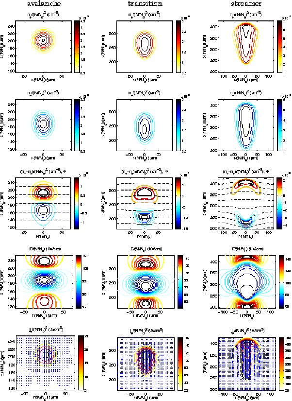
Fig. 1 shows essential features of the solutions that will be substantiated by quantitative analysis in the body of the paper. In the left column, an avalanche can be seen: the electron distribution (upper row) is Gaussian and spherically symmetric. The position of the Gaussian is determined by electron drift in the homogeneous background field, its width by electron diffusion. The ions (second row) are left behind (i.e., further down) and stretched along the temporal trace of the avalanche. The resulting space charge distribution (third row) is essentially a smooth dipole without much structure. Actually, these pictures are quite similar to the sketches of Raether. The electric field (fourth row) is essentially unchanged up to corrections below 1%. The current (lowest row) shows the same Gaussian structure as the electrons; it is dominated by electron drift in the homogeneous background field with a small diffusional correction. In the right column, a conducting filament is formed, and the streamer stage is reached. Electron and ion distribution show a similar long stretched shape. The space charges approach a layered structure, and the field ahead of the streamer is changed by these space charges by up to 40%.
There is some freedom in defining the transition point from avalanche to streamer. In the body of the paper, we will argue that a maximal field enhancement of 3% ahead of the streamer, i.e.,
| (6) |
is a decent measure for the transition. We will see that essentially up to this moment of time the total number of electrons in the avalanche grows exponentially in time, while in the streamer phase, the growth is slower.
1.3 Review of critical field and Raether-Meek criterion
Essentially two criteria have been given in the literature for the emergence of a streamer from a tiny ionization seed, one for the required background field and one for the required space and evolution time. The first one is a necessary lower bound for the background field: the electric field has to be higher than the threshold field where the impact ionization rate overcomes the attachment rate. The ionization level can only grow if the rightmost term in Eq. (1) is positive, hence if the effective ionization coefficient is positive,
| (7) |
This determines the threshold field as
| (8) |
The second criterion is known as the Raether-Meek criterion. It states that the total electron number must have reached the order of to for space charge effects to set in. If this number is reached by exponential multiplication of one initial electron within a constant field , this means that
| (9) |
where is the avalanche length. In brief as a rule of thumb the criterion reads
| (10) |
Let us first note that the same criterion has been suggested for quite different situations in the literature. In his original article, Meek [24] studies the emergence of a cathode directed (i.e., positive) streamer from an anode directed avalanche that has bridged a short gap. On the other hand, Bazelyan and Raizer [25] study the emergence of streamers in free space, i.e. far away from the electrodes. To estimate the field of the ions, Meek used the diffusion radius of the electron avalanche, and the ionization rate in the background field, however, the diffusion does not show up in his transition criterion. Bazelyan and Raizer on the other hand, neglect diffusion and base their criterion on the radius of the avalanche due to electrostatic repulsion. All authors [24, 25, 26, 27] assume the electron distribution to be spherically symmetric, on the other hand, they base their transition criterion on a total field screening, i.e., to in Eq. (6). In view of available simulation results like our Fig. 1, these assumptions are self-contradictory.
Apart from these considerations on the history of the derivation, there are actually two major reasons to revise the Raether-Meek-criterion:
- 1)
The prediction that a parameter should be in the range of 18 to 21 (where authors seem to be willing to assume an even larger range of values to get consistency with experiment) is not very satisfactory and invites improvement.
- 2)
Diffusion has to be included into the model for physical as well as for mathematical reasons. Without diffusion, an initially concentrated electron package would not spread and it would create enormous fields within very short time as they are well known in the neighborhood of point sources. Indeed, diffusion decreases the electron density and the maximal fields while impact ionization increases it. In low fields, diffusion stays dominant for a long time and delays space charge effects and consecutive streamer emergence. It is therefore clear that the avalanche to streamer transition does not only depend on multiplication rates, but also on the relative importance of diffusional spreading. This should provide a more quantitative transition criterion than the pure Raether-Meek criterion.
1.4 Organization of the paper
We will derive a diffusion correction to the Raether-Meek criterion through the following steps: in Section 2, the intrinsic scales of the problem with their explicit density dependence are identified through dimensional analysis. In Section 3, we analyze the spatial distribution of the electrons during the avalanche phase and their contribution to the electric field; this gives a first approximate correction to the Raether-Meek-criterion. In Section 4, we approximate the spatial distribution of the ions and their contribution to the electric field. Electron and ion field are then combined to give the total change of the electric field during the avalanche phase. If this field becomes “substantial” (cf. Fig. 1 and Eq. (6)), we have found the avalanche-to-streamer transition. Finally, the analytical non-dimensional results are translated back to dimensional quantities, and we refer the reader interested in the final prediction only to Figs. 5 and 6 for the transition criterion in non-attaching gases and in air. These figures visualize the analytical criterion (55). Section 5 contains the conclusions, and an additional approximation for the ion generated electric field can be found in the appendix.
2 Dimensional analysis
The Raether-Meek criterion can be understood as a simple example of dimensional analysis. Dimensional analysis identifies general physical properties in terms of dimensionless numbers that are independent of a particular gas type or density. The physical importance of dimensionless numbers like the Reynolds number is well known in hydrodynamics, we here follow the same approach.
In the light of dimensional analysis, the Raether-Meek criterion states that the effective cross-section has the dimension of inverse length, hence the dimensionless number characterizes the gap length in multiples of the ionization length and therefore the exponential multiplication rate . This number directly characterizes the total number of electrons in an avalanche that started from a single free electron. However, this is not the only dimensionless number in the problem, a second one is the dimensionless diffusion constant
| (11) |
that plays a distinctive role in the avalanche to streamer transition as well as it determines the width of the electron cloud. Note that this dimensionless diffusion constant is related to the electron temperature as where is the Boltzmann constant. The electron temperature actually can be defined through this relation, even if the electron energy distribution is not Maxwellian in the presence of strong electric fields. Furthermore, depends on , the two parameters characterizing the Townsend coefficient, given by Eq. (5), for the specific gas and density.
For the general performance of dimensional analysis, we refer to earlier articles [28, 29] and here only state the results: lengths are measured in units of , fields in units of , velocities in units of and time consistently in units of — hence diffusion should be measured in units of as done in (11). The natural scale for the particle densities follows from the Poisson equation, .
The parameters , , and depend on the ratio of the background gas density and the gas density under normal conditions . Using parameters as in [20, 30, 31, 32], the characteristic scales are for N2:
and the dimensionless diffusion constant is . Notice that the characteristic velocity scale is independent of pressure, in agreement with measurements of streamer velocities at different pressures. Notice furthermore, that it directly follows from this analysis that the relevant physical parameter is the reduced electric field .
Dimensionless parameters and fields are introduced as
| (17) |
which brings the system of equations (1)-(4) into the dimensionless form
| (18) | |||||
| (19) | |||||
| (20) |
where the operator is taken with respect to and where is the dimensionless effective ionization rate,
| (21) |
It is remarkable that the density of positive and negative ions enters the equations only in the form of the single dimensionless field . This is clear in the case of the Poisson equation, but holds also for the generation term proportional to . This coefficient accounts for the production of free electrons through impact ionization and for the loss of free electrons due to attachment.
We neglect the effect of photoionization as its rates are typically much lower than impact ionization rates; it does not contribute significantly to the build-up of a compact ionized cloud where eventually space charge effects will set in (quite in contrast to its distinct role in positive streamer propagation).
3 Electron distribution and field
We derive the transition as follows: We assume that an avalanche starts from a single electron and follows a transition as shown in Fig. 1. In the calculation we neglect space charge effects on the evolution of densities, but we do calculate the additional electric field generated by the space charges. If this field reaches a relative value of k=0.03 — this value will be motivated in Section 4.3 —, space charge effects are not negligible anymore, and the transition to the streamer is found.
The electric field generated by space charges has one contribution from the electrons and another one from the positive and negative ions . In the present section, we calculate the field of the electrons, in the next section, we will include the field of the ions.
3.1 The electron distribution: a Gaussian
We write the single electron that generates the avalanche as a localized initial density
| (22) |
and consider its evolution under influence of a uniform field , where is the unit vector in the direction and is constant. A single electron is written as a -function in physical units where the spatial integral over the electron number density
| (23) |
of course, should be unity . According to the last section, this corresponds in dimensionless units to which is for nitrogen. We will use in the sequel. We emphasize, however, that the theory will be developed for an arbitrary value of .
During the avalanche phase the electric field remains unaffected by space charges, so that the continuity equations for the charged particles (18)-(19) can be linearized around the background field,
| (24) | |||||
| (25) |
where .
For the initial condition (22), the electron evolution according to Eq. (24) can be given explicitly as [20]
| (26) |
it has the form of a Gaussian package that drifts with velocity , widens diffusively with half width proportional to , and carries a total number of electrons . (If the initial ionization seed consists of several electrons in some close neighborhood, the Gaussian shape is approached nevertheless for large times due to the central limit theorem.)
Integrating Eq. (26) over the entire space shows that the total number of electrons grows as (if we start with a single electron). On the other hand, the maximum of the electron density is reached at the center of the Gaussian and has the value
| (27) |
hence it first decreases until due to diffusion and then increases due to electron multiplication. At this moment of evolution, generation overcomes diffusion.
The axial electron density distribution for a background field of at (for N2 this corresponds to a reduced electric field kV/cm and =6 ns) is illustrated in the upper panel of Fig. 2. The analytical solution (26) of the linearized continuity equation (24) is compared to a numerical evaluation of the full nonlinear problem (18)-(20). The excellent correspondence between the solution of both the linearized and the nonlinear problem shows that, at this time, space charge effects are negligible, so that the electrons still are in the avalanche phase.

3.2 Exact result for the electron generated field
While density and field of the ions can only be calculated approximately and will be treated in the next section, the electric field generated by the Gaussian electron package can be calculated exactly.
The main point is that the electron density distribution (26) is spherically symmetric about the point . The electric field at the point
| (28) |
can therefore be written as , where is the unit vector in the radial direction. Its magnitude can be computed with Gauss’ law of electrostatics (in the same way as the gravitational force field of a spherically symmetric mass distribution). It uses the fact that the field at radius is determined by the total charge inside the sphere of radius , and independent of charges outside this radius, as long as the distribution is spherically symmetric. It yields
| (29) |
with
| (30) |
where erf is the error function.
The spatial maximum of the field strength is determined by the maximum of ; evaluating shows that it is located at an such that
| (31) |
Solving this equation numerically leads to a position of the maximum of about (which is the radius at which the Gaussian electron distribution has dropped to of its maximal value) and to the value . The spatial maximum of the electron generated electric field strength becomes
| (32) |
it is located on the sphere parameterized through
| (33) |
In the original cylindrically symmetric coordinate system , the axial field component is directed in the negative -direction, i.e. in the same direction as the background field, “ahead” of the electron cloud () as is illustrated by the solid line in the lower panel of Fig. 2. Combining this with Eq. (33), we find that the maximal field strength and its location are
| (34) | |||
| (35) |
3.3 A lower bound for the transition
Since the avalanche to streamer transition takes place when space charge effects start to affect the electric field, we choose to base the criterion for the transition on the maximal relative field enhancement defined in Eq. (6), which for the dimensionless field simply reads
| (36) |
Here is the total electric field, and being the fields of the electrons and the ions, respectively. We will show in the next section that is an appropriate estimate for the maximal relative field enhancement at the mid gap avalanche to streamer transition. At lower values of , space charge effects can be neglected, whereas at higher values the dynamics of the electrons are nonlinear and the full streamer equations (26)-(20) have to be solved.
As a first estimate for the space charge field, and thereby for the avalanche to streamer transition, we compute the field generated by the electrons only and neglect the ion field. This is a decent approximation, as the lower panel in Fig. 2 shows. Actually, the magnitude of the monopole field ahead of the electron cloud is an upper bound for the magnitude of the field created by the dipole of electrons on the one hand and the positive charges left behind by the electron cloud on the other hand. Therefore, the maximal relative field enhancement due to the electrons, , exceeds the transition value after a shorter travel time and distance then the genuine relative field enhancement of Eq. (36). Hence, is a lower bound for the time of the avalanche-to-streamer transition.
The lower bound for the transition can be expressed through Eq. (32) as
| (37) |
As travel time and travel distance are related through the drift velocity , is found to be identical to in dimensional units where is the avalanche travel distance. In dimensional quantities, Eq. (37) takes the form
| (38) |
For a non-attaching gas () at atmospheric pressure under normal conditions with dimensionless diffusion comparable to nitrogen, inserting the numerical values for the parameters, we obtain
| (39) |
being a growing function of , Eq. (37) shows that the larger the field, the earlier the transition takes place, which is in accordance with Meek’s criterion. On the other hand, the second term on the right hand side of Eq. (38) depends on the diffusion coefficient in such a way that diffusion delays the transition to streamer, as expected.
The solution for at atmospheric pressure is shown in the dash-dotted line of Fig. 3, where it is compared to a numerical evaluation of the transition time (circles). The latter have been obtained through a full simulation of the continuity equations (18)-(19) together with the Poisson equation (20) [29, 21] that was also used to generate Fig. 1. Though the qualitative features of the transition time are well reproduced, this figure shows that the underestimation of the transition time is significant, and that it is necessary to include the field of the ion trail left behind by the electrons.

4 Ion distribution and field
4.1 Exact results on the spatial moments of the distributions
To get a more accurate estimate for the avalanche-to-streamer transition, the field generated by the positive and negative ions has to be included. In the case of the ion distribution, closed analytical results cannot be found, in contrast to the electron distribution (26). However, arbitrary spatial moments of the distribution
| (40) |
can be derived analytically. Here is the direction of the homogeneous field and is the radial direction. First, the evolution equation (19) for the ion density is integrated in time and the analytical form (26) for is inserted. As is constant in space and time one finds
| (41) | |||
Here the initial perturbation is located at on the axis . The moments (40) can now be derived from (41) by exchanging the order of spatial and temporal integration. In particular, one finds
| (42) | |||||
and higher moments can be calculated in the same way. For the moments of in the axial direction, this gives
| (43) | |||||
| (44) |
The second moment of in the radial direction is
| (45) |
For comparison, the moments of the Gaussian electron distribution (26) are easily found to be
| (46) | |||||
| (47) | |||||
| (48) |
4.2 Discussion of the moments
Let us now interprete these moments. A first moment of a spatial distribution gives its center of mass. For the second moment, the cumulant
| (49) |
measures the quadratic extension from the center of mass. As the center of mass lies on the axis, for the radial extension the distinction between second moment and its cumulant need not be made.
The moments for the electrons (46)–(48) have a simple structure: the center of mass of the electron package is located at , and the package has a diffusive width around it, both in the forward direction and in the radial direction.
The ion cloud shows a more complex behavior; it is evaluated close to the avalanche-to-streamer transition where , therefore the terms of order are neglected.
First it is remarkable that the center of mass of the ion cloud (43) shifts with precisely the same velocity as the electron cloud though the ion motion is neglected while the electrons drift, therefore the ion center of mass is at an approximately constant distance behind the electron center of mass. This distance
| (50) |
corresponds to the dimensional ionization length .
The quadratic radial width of the ion cloud is smaller than the one of the electron cloud. This is related to the fact that the electron cloud also was more narrow at the earlier times when it left the ions behind. The ion cloud is more extended in the direction. More precisely, its length is larger than its width. This comes from the ions being immobile, therefore a trace of ions is left behind by the electron cloud. Moreover, it can be remarked that the difference between quadratic width and length of the ion cloud is given by the same ionization length as the distance between the centers of mass of the ion and the electron cloud. We refer to the left column of Fig. 1 for the illustration of these density distributions.
4.3 An estimate for the transition
One can assume as in [25] that the ions have a spatial distribution similar to the electrons, thus a Gaussian with the same width as the electron cloud, but centered around :
| (51) |
In this approximation, the total electric field becomes:
| (52) |
where
| (53) |
are the distances to the electron and ion centers of mass.
The maximum of the field can not be computed analytically. However, in Fig. 1 and in the lower panel of Fig. 2, it can be seen that this maximum is located on the axis ahead of the electron cloud, and that the location of the maximum of the total field and that of the electron field nearly coincide. This can easily be explained physically: the total field is the sum of the fields induced by the electrons and by the ions. Its maximum is located just ahead of the electron cloud, where the electron field varies rapidly, while the field contribution of the ions is smoother and smaller as we are interested in its contribution further away from the center of the ion distribution. Therefore the maximum position of the total field is essentially identical to the maximum position of the electron field. This justifies our approximation to evaluate the field at the maximum position of as defined in Eq. (35). The maximum of the electric field can thus be approximated as:
| (54) |
Then implies for the transition time :
| (55) |
where is defined in Eq. (30). The argument of the logarithm in the third term on the left hand side is larger than 1, therefore this criterion gives a later transition time than that based on the field of the electrons only. This is what we expect considering that the ions tend to reduce the field of the electrons, thus the effect of space charge. The correction given by the ion field is a function of the ratio of the ionization length and the diffusion length . At early times, this ratio goes to infinity, and the correction given by the ion cloud is negligible. However, at later times, the correction becomes more significant.
4.4 The analytically approximated transition criterion compared with numerical results
We now compare again our analytical results for the linearized problem to the outcome of numerical simulations of the full nonlinear model (18)-(20).
In the upper panel of Fig 4 the evolution of the maximal electron density as a function of is shown.

Upper panel: the evolution of the maximal electron density as a function of as computed within the full nonlinear 2D model (solid lines) and as given by the analytical solution (27) of the linearized problem (dash dotted lines).
Lower panel: the evolution of the maximal electric field enhancement as a function of . Solid lines: numerical solution of the full nonlinear 2D model; dashed dotted lines: only the field of the electrons is accounted for in the analysis, see Eq. (32); dashed lines: analytical approximation (54) of the total field.
Numerical and analytical solutions coincide during the avalanche phase, but deviate eventually. This enables us to estimate the moment at which the space charge effects set in, and thus when the streamer regime is reached. In the lower panel of Fig 4 the evolution of the maximal relative field enhancement is considered. Looking at the simulation results (the solid lines), we see that gives a good estimate of the transition time.
The approximation (54) for the maximal field has now become much better than the previous approximation (32) based on the electron cloud only. Indeed, for e.g the case of (corresponding to the medium thick lines), the numerically computed field (solid line) reaches the transition value ( at . When only the field of the electrons is taken into account, this value would already be reached at , while the correction based on the approximation of the ion cloud leads to a transition time of . The correction becomes especially important at higher fields. In low fields, the approximation of the ions shows somewhat larger deviations. We notice that the analytical approximation is narrower and higher than the genuine one, and therefore leads to an overestimation of the field generated by the ions inside the ion cloud. For an even more accurate estimate of the total field between the electron and the ion cloud we refer to Appendix 2, where it is also shown this will not lead to a significant improve in the estimate of the maximal field ahead of the electron cloud.
In Fig. 3 we compare the transition times given by Eqs. (37) and (55) with numerically evaluated transition times. It shows that the approximation of similar electron and ion distributions leads to a very good approximation of the transition time. This figure also illustrates that the transition time depends strongly on the electric field, and increases for smaller fields. Moreover, looking at the transition time for higher diffusion coefficients, it is seen that diffusion tends to delay the transition to the streamer regime. This can be expected, since diffusion will tend to broaden the electron cloud, thereby suppressing space charge effects. Depending on the external parameters, the value of at the time the transition takes place can vary by a factor two or more.
4.5 The final results on the transition criterion
The transition time approximated by Eq. (55) as a function of both background electric field and diffusion coefficient is visualized as the 3-dimensional in Fig. 5. This figure shows that the Raether-Meek transition criterion, that stated that takes an approximately constant value of 18 to 21, corresponds to the case of relatively high diffusion and background field. However, realistic values of are smaller than unity, and a background electric field higher than 2 also leads to unrealistic values. So in the parameter range of real experiments, the correction given by Eq. (3) on the Raether-Meek criterion can not be neglected.

We no discuss the particular example of an electron avalanche in (dry) air, for which different coefficients have to be used than in N2. In particular, the ionization length and field in air are given by [20] and . For the values of the mobility and the diffusion coefficient of the electrons as a function of the electric field we use experimental values as well as numerical solutions of the Boltzmann equation (see Appendix A). Inserting those in Eq. (55), we can compute the value of at the transition for different background fields, showed in Fig. 6. At large fields, the value of at transition saturates towards 16, and grows asymptotically as the reduced field approaches a value of 27.7 kV/cm. At even lower fields attachment overcomes electron impact ionization, and a single electron can not generate a streamer. Large values of as in Fig 5 are not found, as electron attachment limits the emergence of streamers in low fields (see Eq. (8)). So for air, drops from 21 to 15 with growing field.

5 Summary and conclusions
Recent simulations (see Fig. 1) have shown that an electron avalanche turns into a streamer when the field enhancement due to space charges is about 3%. In this paper, the theory behind the commonly used Raether-Meek criterion is reviewed, as it assumes a linear behavior of the electrons (i.e. space charge effects can be neglected), which is in contradiction with the requirement of the space charge field to be in the same order of magnitude as the background field for the transition to occur.
A dimensional analysis has been carried, enabling us to identify the characteristic length scales, which are a function of the neutral gas density. In particular, the dimensionless quantities and have been extracted from the problem. The first gives the distance in multiples of the effective ionization length in the background field, while the latter gives the ratio between diffusive and advective transport of electrons. The continuity equations for the positive and negative ions (2)-(3) reduce to one single equation (19) holding both positive and negative ions after rescaling, making the further analysis valid for both attaching gases like air or non-attaching gases like N2 or Ar.
The avalanche regime was identified as the phase during which space charge effects are negligible. This implies that the problem can be linearized around the background field, making it well-suited for analytical treatment. Indeed, for an electron avalanche evolving in a homogeneous background electric field, a closed analytical expressions exist for the density distribution of the electrons. Comparing this analytical solution of the linearized problem to the results of a numerical simulation of the full nonlinear problem, it could be concluded that the transition to streamer takes when the maximal relative field enhancement has reached a value of approximately 3%.
We have shown that the electric field of the electron cloud during the avalanche regime can also be described by a closed expression. This led to the derivation of a lower bound for the avalanche to streamer transition (37). The estimate of the transition time has been improved by taking into account the field of the ions for which, in contrast to the electrons, no closed expression exists. However, the contribution of the ions to the maximal relative field enhancement can be well approximated. leading to an analytical estimate of the avalanche to streamer transition (55).
The transition distance strongly depends on diffusion and on the background electric field. For high fields, the transition time saturates towards . On the other hand, for low fields, when the processes are diffusion dominated, the avalanche lasts longer. We remark that the striations observed in [15] are generic for atomic gasses with essentially only elastic and ionizing collisions, i.e. with very few inelastic processes [35].
In air, attachment limits the emergence of a streamer in low fields (see Eq. (8)). In this case, at transition is in the range of 16 (for high background fields) to 21 (for fields approaching ). It is remarkable that in the end, due to attachment cut-offs, Meek’s criterion performs quite good for the emergence of streamers in free space. In non-attaching gases like N2 or Ar, the correction on Meek’s criterion, that stated that , becomes important at low fields. There the relatively strong diffusion delays the transition to streamer considerably. We emphasize that the use of dimensionless quantities enable us to translate the criterion given in (55) to any given neutral gas type and density. Evaluating the characteristic scales for these conditions, dimensionless field and diffusion can be computed, and the value of at transition can be computed from Eq. (55) or read from Fig. 5. Actually, Fig. 5 can also be used for attaching gases, as long as the ionization threshold field is accounted for.
The analytical models presented in this paper give a useful tool to describe the streamer formation. We stress that our criterion for the transition is based on a significant contribution of the space charges on the background electric field. Our analysis fully relied on the linearization of the streamer equations around the background field. The nonlinear streamer propagation is the subject of other studies. In that phase the space charges and electric field strongly interact, and the analytical study of such streamers [36] is far more difficult than the analysis of the linear avalanche phase.
Appendix A Mobility and diffusion coefficients of electrons in air
To compute the transition time in air, we use values of the electron mobility and diffusion coefficient found in literature. In the left plot of Fig. 7 measured and calculated values of are given, as well as the fit are shown. The experimental values have been found in the survey of electron swarm data by Dutton [33]. The computed values are the solution of the Boltzmann equation and have been taken from [5]. Also, the empirical approximation of the ionization coefficient as a function of the background field as given by [20] is shown, with and .
The values of as a function of the reduced electric field are given in the right plot of Fig. 7. Again, computed values from [5] are shown, as well as measured values found in [34]. The value of the diffusion coefficient as a function of the electric field can obviously easily be derived from these figures.


Appendix B A more accurate approximation for the ion density distribution
The approximation for the ion distribution in Sect. 4 leads to a relatively good approximation for the transition time in the case of a mid-gap transition. However, the real spatial distribution of ions is more narrow in the -direction, and can be wider and asymmetrical in the -direction. In this appendix we present another approximation for the ion distribution, which will lead to a better overall approximation of the electric field, and of the self field induced by the ion trail. The price however to pay for this is a much more complicated analytical expression for the density and the field.
A better approximation for would then be an ellipsoidal Gaussian distribution centered around with width and in the - and -direction, respectively. The height of this Gaussian should be such that the total amount of ions at time is still equal to . The appropriate expression for the ion distribution is:
| (56) |
However, as far as we know, no closed analytical expression is known for the field of such an ellipsoidal Gaussian charge distribution. So instead, we take a spherical Gaussian distribution with the same height as the one defined in Eq. (56):
| (57) |
where
| (58) | |||||

In Fig. 8 we compare the densities and fields given by the numerical solution and and . It shows clearly that the approximation does not give a better approximation of the field ahead of the electron cloud. This can be explained by the fact that, the region ahead of the electron cloud does not contain any ions, so that the field induced by the ions is only a function of the total number of ions, which is the same in both and . On the other hand, inside the ion cloud the approximation is much better. Therefore, evaluating the electron and ion densities with Eqs. (26) and (57) and their fields with Eqs. (29) and (59), at the transition time given by Eq. (55), will give a good approximation of the status of the process at the time that streamer regime is entered.
References
References
- [1] V. Mazur, P.R. Krehbiel, and X. Shao. Correlated high-speed video and radio interferometric observations of a cloud-to-ground lightning flash. J. Geophys. Res., 100:25731–25754, 1995.
- [2] E.M. Bazelyan and Yu.P. Raizer. Lightning Physics and Lightning Protection. Institute of Physics Publishing, Bristol, U.K., 2000.
- [3] E.A. Gerken, U.S. Inan, and C.P. Barrington-Leigh. Telescopic imaging of sprites. Geophys. Res. Lett., 27:2637, 2000.
- [4] V.P. Pasko and H.C. Stenbaek-Nielsen. Diffuse and streamer regions of sprites. Geophys. Res. Lett., 29:82(1–4), 2002.
- [5] N. Liu and V.P. Pasko. Effects of photoionization on propagation and branching of positive and negative streamers in sprites. J. Geophys. Res, 109:A04301(1–17), 2004.
- [6] F.F. Chen. Industrial applications of low-temperature plasma physics. Phys. Plasmas, 2:2164–2175, 1995.
- [7] B. Eliasson and U. Kogelschatz. Modeling and applications of silent discharge plasmas. IEEE Trans. Plasma Sci., 19:309–323, 1991.
- [8] K. Shimizu, K. Kinoshita, K. Yanagihara, B.S. Rajanikanth, S. Katsura, and A. Mizuno. Pulsed-plasma treatment of polluted gas using wet-/low-temperature corona reactors. IEEE Trans. Plasma Sci., 33:1373–1380, 1997.
- [9] I.V. Lisitsyn, H. Nomiyama, S. Katsuki, and H. Akiyama. Streamer discharge reactor for water treatment by pulsed power. Rev. Sci. Instr., 70:3457–3462, 1999.
- [10] G.J.J. Winands, K. Yan, A. Nair, A.J.M. Pemen, and E.J.M van Heesch. Evaluation of corona plasma techniques for industrial applications: HPPS and DC/AC systems. Plasma Proc. and Polymers, 2:232–237, 2005.
- [11] M. Makarov, J. Bonnet, and D. Pigache. High efficiency discharge-pumped XeCl laser. Appl. Phys. B, 66:417–426, 1998.
- [12] A. Oda, H. Sugawara, Y. Sakai, and H. Akashi. Estimation of the light output power and efficiency of Xe barrier discharge excimer lamps using a one-dimensional fluid model for various voltage waveforms. J. Phys. D: Appl. Phys., 33:1507–1513, 2000.
- [13] U. Kogelschatz. Industrial innovation based on fundamental physics. Plasma Sources Sci. Technol., 11:A1–A6, 2002.
- [14] U. Ebert, C. Montijn, T.M.P. Briels, W. Hundsdorfer, B. Meulenbroek, A. Rocco, and E.M. van Veldhuizen. The multiscale nature of streamers. http://arxiv.org/abs/physics/0604023 , to appear in Plasma Sources Science and Technology, 2006.
- [15] B.J.P. Dowds, R.K. Barrett, and D.A. Diver. Streamer initiation in atmospheric pressure gas discharges by direct particle simulation. Phys. Rev. E, 68:026412(1–9), 2003.
- [16] C.T. Phelps and R.F. Griffiths. Dependence of positive corona streamer propagation on air pressure and water vapor content. J. Appl. Phys., 47:2929–2934, 1976.
- [17] J.R. Dwyer. A fundamental limit on electric fields in air. Geophys. Res. Lett., 30:2055, 2003.
- [18] A.V. Gurevich and K.R. Zybin. Runaway breakdown and the mysteries of lightning. Physics today, 58:37–43, 2005.
- [19] H. Raether. The development of electron avalanche in a spark channel (from observations in a cloud chamber). Z. Phys, 112:464, 1939.
- [20] Y.P. Raizer. Gas Discharge Physics. Springer, Berlin, 1991.
- [21]
C. Montijn, W. Hundsdorfer, and U. Ebert.
An adaptive grid method for the simulations of negative streamers in
nitrogen.
http://arxiv.org/abs/physics/0603070 , submitted to J. Comp. Phys., 2006. - [22] C. Montijn. Evolution of negative streamers in nitrogen: a numerical investigation on adaptive grids. PhD thesis, Tech. Univ. Eindhoven, 2005.
- [23]
C. Montijn, U. Ebert, and W. Hundsdorfer.
Numerical convergence of the branching time of negative streamers.
http://arxiv.org/abs/physics/0604012 , submitted to Phys. Rev. E, 2006. - [24] J.M. Meek. A theory of spark discharge. Phys. Rev., 57:722–728, 1940.
- [25] E.M. Bazelyan and Yu.P. Raizer. Spark discharge. CRC Press, New York, 1998.
- [26] L.B. Loeb and J.M. Meek. The mechanism of spark discharge in air at atmospheric pressure. I. J. Appl. Phys., 11:438–447, 1940.
- [27] L.B. Loeb and J.M. Meek. The mechanism of spark discharge in air at atmospheric pressure. II. J. Appl. Phys., 11:459–474, 1940.
- [28] U. Ebert, W. van Saarloos, and C. Caroli. Propagation and structure of planar streamer fronts. Phys. Rev. E, 55:1530–1549, 1997.
- [29] A. Rocco, U. Ebert, and W. Hundsdorfer. Branching of negative streamers in free flight. Phys. Rev. E, 66:035102(1–4), 2002.
- [30] S.K. Dhali and P.F. Williams. Two-dimensional studies of streamers in gases. J. Appl. Phys, 62:4696–4706, 1987.
- [31] P.A. Vitello, B.M. Penetrante, and J.N. Bardsley. Simulation of negative-streamer dynamics in nitrogen. Phys. Rev. E, 49:5574–5598, 1994.
- [32] A.J. Davies, C.S. Davies, and C.J. Evans. Computer simulation of rapidly developing gaseous discharges. Proc. IEE, 118:816–823, 1971.
- [33] J. Dutton. A survey of electron swarm data. J. Phys. Chem. Ref. Data, 4:664, 1975.
- [34] C.S. Lakshminarasimha and J. Lucas. The ratio of radial diffusion coefficient to mobility for electrons in helium, argon, air, methane and nitric oxide. J. Phys. D: Appl. Phys., 10:313–321, 1977.
- [35] W.M.B. Brok. Modelling of transient phenomena in gas discharges. PhD thesis, Tech. Univ. Eindhoven, 2005.
- [36] B. Meulenbroek, A. Rocco, and U. Ebert. Streamer branching rationalized by conformal mapping techniques. Phys. Rev. E, 69:067402(1–4), 2004.