Parity nonconservation in Atomic Zeeman Transitions
Abstract
We discuss the possibility of measuring nuclear anapole moments in atomic Zeeman transitions and perform the necessary calculations. Advantages of using Zeeman transitions include variable transition frequencies and the possibility of enhancement of parity nonconservation effects.
pacs
32.80.Ys, 32.60.+i, 24.80.+yExperiments on parity nonconservation in atoms have measured the electron-nucleon weak interaction and have provided very accurate tests of the Standard Model at low energies (see, e.g., review GF). It has been pointed out in Ref. Flambaum that atomic experiments can be used to measure the nuclear anapole moment and study parity nonconserving (PNC) nuclear forces. The measurement of the anapole moment of 133Cs nucleus was reported in Ref. Wieman. However, the strength of the PNC nuclear forces extracted from this measurement seem to disagree with the limits on these forces extracted from the 205Tl anapole measurement performed in another atomic experiment Fortson. Moreover, the general situation with PNC nuclear forces at the moment is controversial since different experiments give contradictory results (see, e.g., review GF). This situation requires new measurements of nuclear anapole moments.
The PNC interaction in atoms can be split into a nuclear spin-dependent (NSD) and nuclear spin-independent (NSI) part. The NSI part is due to the nuclear weak charge, and the PNC effects produced by the NSI part are two orders of magnitude larger than the PNC effects produced by the NSD part. There are three contributions to the NSD part of the PNC interaction: the nuclear anapole moment, the NSD part of the electron-nucleus interaction, and the combination of the NSI electron-nucleus weak interaction and the hyperfine interaction. For heavy atoms the anapole moment contribution dominates since it grows as Flambaum; FSK; FK. In experiments Wieman; Fortson the NSD contribution was separated from the much larger NSI contribution. The NSD contribution is different in different hyperfine components of an optical transition and can be extracted from the difference of the PNC effects in these components. An alternative method to measure the NSD interaction was suggested in Ref. Khriplovich_1975. The NSI part is zero in transitions between hyperfine terms of a ground state electronic level. The measurements of PNC in the hyperfine transitions is sensitive to the NSD PNC interaction only. Unfortunately, no such experiment has been performed.
It was suggested in Refs. Zeeman (see also review Budker and references therein) that the transitions between the Zeeman components of the hyperfine levels of a ground state atom in a magnetic field may be more convenient for the measurements of PNC induced by the NSD interaction, than transitions between the hyperfine levels themselves. The NSI interaction still does not contribute here, therefore, the measurement of the PNC effects in Zeeman transitions can provide a value of the nuclear anapole moment. One advantage of using these transitions is that for weak external magnetic fields, the transition frequency is proportional to the field and so can be chosen arbitrarily small, and determined from the conditions required for optimal experimental setup. Advantages of the low frequency were explained in the proposal of possible experiments in hydrogen, potassium and cesium hyperfine transitions Gorshkov. At low frequencies one does not need a resonator to produce the electromagnetic field. This greatly simplifies the experiment and allows the frequency to be set to the same value for different atoms. It should be noted that the PNC E1 amplitudes of the Zeeman transitions in weak magnetic fields are suppressed by a factor , where is the transition frequency and is the hyperfine splitting. However, the E1 amplitude increases with nuclear charge as , where is a relativistic correction factor (see, e.g. Khriplovich; GF ), while the hyperfine splitting increases as . Combining these results we can see that the E1 amplitude of Zeeman transitions increases faster than for heavy atoms in weak magnetic fields at a fixed transition frequency. This suggests that heavy atoms should be considered as candidates for an experiment.
Another possible advantage appears for Zeeman transitions in a strong magnetic field Zeeman; Gorshkov. Parity nonconservation appear due to interference between the PNC electric dipole amplitude, , and the magnetic dipole amplitude, , . In a strong magnetic field an eigenstate is approximately a product of the nuclear spin state times the electron wave function. The amplitude, , between the Zeeman states corresponding to nuclear spin-flip is very small, since the nuclear magnetic moment is 1000 times smaller than the electron magnetic moment (in reality the contribution from the small admixture of the state with a different electron angular momentum projection will always dominate ). The magnitude of the PNC amplitude, , is not suppressed for such transitions. This enhances the value of PNC effects () containing in the denominator.
In this paper we will consider three different experimental schemes: no magnetic field, a weak magnetic field (), and a strong magnetic field (). For each we shall calculate the ratio , where is the PNC E1 amplitude, is the M1 amplitude and is the transition frequency. A promising transition will have a relatively large , since the PNC E1 amplitude, , will be large, the background parity conserving M1 amplitude, , will be relatively small, and ideally the transition frequency should also be low, as mentioned previously.
We consider atoms and ions with the electron angular momentum . In this case the only allowed values for the total atomic angular momentum are , where is the nuclear spin. In the presence of a magnetic field, states with a fixed are split into states with a fixed projection, , onto the external field direction. The total angular momentum is no longer conserved, there is a mixing of states with the same projection, , resulting in the appearance of the new states:
| (1) | |||||
| (2) |
The mixing coefficients, , in these equations are calculated from the secular equations with the hyperfine interaction and the interaction with the external magnetic field taken together. In the low field limit
In the high field limit the coupling between and is broken and it is no longer proper to consider the states in terms of , instead we need to consider them in terms of and . In this limit we have the states
It makes no sense to divide the terms into hyperfine and Zeeman transitions in the high field limit because is not conserved, nevertheless we shall call the transitions the hyperfine ones and the , and the Zeeman ones.
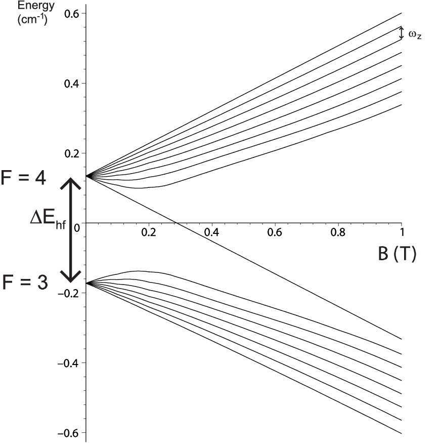
The dependence of the 133Cs energy levels on the external magnetic field is presented in Figure 1. In weak magnetic fields the energy difference of the hyperfine term and is constant and equal to while the energy difference of the Zeeman terms is proportional to the field. In the strong field the hyperfine transition energy increases in proportion to the field while the Zeeman transition energy is constant and equal to . Here and below we neglect small terms where is the nuclear magnetic moment.
For the hyperfine transitions without the external field the ratio is given by
| (3) | |||||
Here is the atomic magnetic (Landé) -factor: for the valence electron (K, Rb, Cs, Ba+, Au, Fr), and for the valence electron (Tl).
In weak fields the E1 amplitudes behave just like the transition frequencies (they are proportional to the field for Zeeman transitions and constant for hyperfine ones), while the M1 amplitudes are independent of the weak field. The parameters, given by
for hyperfine transitions are independent of the field while it is weak. For Zeeman transitions they are given by
| (4) | |||
| (5) |
Here we use spherical components of the electric and magnetic dipole operators defined as and .
In strong magnetic fields the transitions are not interesting since the transition corresponds to , resulting in the E1 amplitude being forbidden due to selection rules, while for the transition both the M1 and E1 amplitude are independent of the magnetic field and so the magnetic field dependence of comes entirely from which increases linearly with magnetic field, resulting in decreasing inversely to the magnetic field. By contrast, in the transition the E1 amplitude is independent of the external magnetic field. The parameter can also be shown to be independent of the field and always equal to . The E1 amplitude of the Zeeman transitions in a strong magnetic field reach a constant value, comparable to the E1 amplitude of the hyperfine transitions. The frequencies also reach a constant value, given by , while the M1 transition amplitudes decrease in proportion to the field. This results in the R parameters increasing with the field
| (6) | |||||
where .
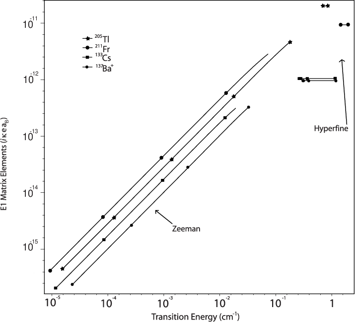
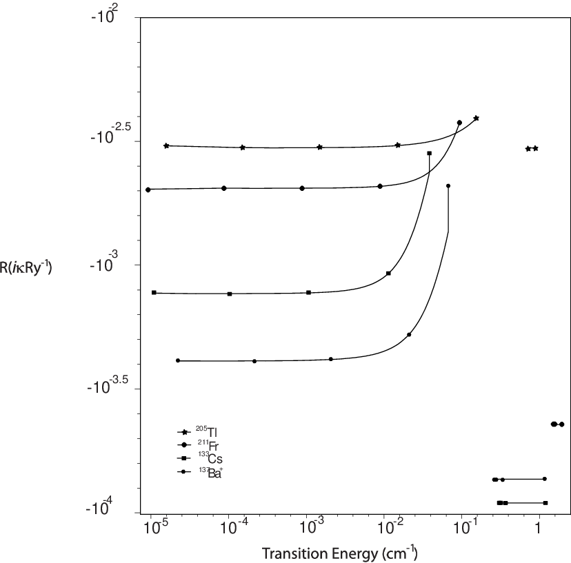
Calculated parameters for a collection of atoms are presented in Table 1. In Tables 2, 3 and 4 we present , and for the different magnetic fields. The dimensionless coupling constant, , consisting mainly of the anapole moment of the nucleus has been left as a free parameter, we present an estimate of in Table 3 to give an approximation of the size of this term. The P-odd E1 transition amplitudes, , parameter and transition frequencies, all depend upon the magnetic field, but it is useful to consider and as a function of . These relationships are presented in Figures 2 and 3. Moving from left to right in these graphs corresponds to an increasing magnetic field. These figures show that for transitions with the same frequency, Zeeman transitions have a larger P-odd E1 amplitude as well as a larger ratio of the E1 amplitude to the P-even M1 amplitude than the hyperfine transitions.
We conclude that Zeeman transitions in heavy atoms have some advantages over the hyperfine transitions that have been considered previously. The biggest advantage is that the transition frequencies can be tuned to make an experiment easier to perform, increase sensitivity and provide additional control of systematic effects by varying the magnetic field. Zeeman transitions should be considered as candidates for experiments to measure the anapole moment of nuclei.
| Atom/ion | I | R () | ||||||
|---|---|---|---|---|---|---|---|---|
| 39K | 1.5 | 1-2 | 0.015411 1 Reference Happer | -1.18 | -0.85 | -2.5 | -3.4 | |
| 85Rb | 2.5 | 2-3 | 0.10122 2 Reference Vanier | -8.74 | -0.76 | -3.8 | -4.6 | |
| 87Rb | 1.5 | 1-2 | 0.22833 3 Reference Bize | 7.27 | 0.35 | 1.1 | 1.4 | |
| 133Cs | 3.5 | 3-4 | 0.30711 1 Reference Happer | -43.8 | -1.1 | -7.6 | -8.6 | |
| 137Ba+ | 1.5 | 1-2 | 0.26844 4 Reference Blatt | -32.9 | -1.3 | -4.0 | -5.4 | |
| 197Au | 1.5 | 1-2 | 0.20355 5 Reference Dahman | 85.4 | 4.6 | 14. | 18. | |
| 205Tl | 0.5 | 0-1 | 0.7166 6 Reference Lurio | -40088 8 A significantly different value of -141 was obtained for this reduced matrix element in Kozlov1. | -29. | -29. | -59. | |
| 211Fr | 4.5 | 4-5 | 1.45177 7 Reference Lieberman | -48199 9 A similar value of -445 was calculated in Kozlov2. | -2.2 | -20. | -22. | |
| Atom/ion | B=0 | ||
|---|---|---|---|
| theory | |||
| 39K | 0.0154 | 0.0039 | 0.0039 |
| 85Rb | 0.101 | 0.0168 | 0.0168 |
| 87Rb | 0.228 | 0.0570 | 0.0570 |
| 133Cs | 0.307 | 0.0384 | 0.0384 |
| 137Ba+ | 0.268 | 0.0670 | 0.0670 |
| 197Au | 0.203 | 0.0508 | 0.0508 |
| 205Tl | 0.71 | 0.355 | 0.355 |
| 211Fr | 1.451 | 0.1451 | 0.1451 |
| Atom/ion | 11 1 These are calculated using the formula , where is the fine structure constant, is the magnetic moment in nuclear magnetons of the external nucleon (a proton for all the cases above), is the mass of the external nucleon (ie proton mass), fm, and is the strength of the weak nuclear potential in units of the Fermi constant . More details about how anapole moments can be calculated can be found in the review GF. | 22 2 These are calculated using the expression, . | transition33 3 These shows which Zeeman transitions have the largest E1 amplitude in a small field. I stands for the transition and II stands for the transition . It should be noted that the difference between these amplitudes is very small. | 44 4 These are calculated using the expression, , where . | 55 5 These are calculated with the expression, . |
| 39K | 0.17 | I | |||
| 85Rb | 0.28 | I | |||
| 87Rb | 0.28 | I | |||
| 133Cs | 0.38 | I | |||
| 137Ba+ | 0.38 | I | |||
| 197Au | 0.49 | I | |||
| 205Tl | 0.50 | II | |||
| 211Fr | 0.51 | II |
| Atom/ion | 11 1 These are calculated using the expression . | 22 2 These are calculated using the expression . | 33 3 These are calculated using the expression where . |
|---|---|---|---|
| 39K | |||
| 85Rb | |||
| 87Rb | |||
| 133Cs | |||
| 137Ba+ | |||
| 197Au | |||
| 205Tl | |||
| 211Fr |
References
- (1) J.S.M. Ginges, V.V. Flambaum. Phys. Rep. 397, 63 (2004).
- (2) V. V. Flambaum and I. B. Khriplovich, Sov. Phys. -JEPT 52, 835 (1980).
- (3) C.S. Wood, S.C. Bennet, D. Cho, B.P. Masterson, J.L. Roberts, C.E. Tanner, C.E. Wieman. Science 275,1759 (1997).
- (4) P.A. Vetter, D.M. Meekhof, P.K. Majumder, S.K. Lamoreaux, E.N. Fortson. Phys. Rev. Lett 74, 2658 (1995).
- (5) V. V. Flambaum, I. B. Khriplovich, and O.P. Sushkov. Phys. Lett. B146, 367 (1984).
- (6) V. V. Flambaum and I. B. Khriplovich, Sov. Phys. -JEPT 62, 872 (1985).
- (7) V. N. Novikov and I. B. Khriplovich, JEPT Lett. 22, 74 (1975).
- (8) V.V. Flambaum, 1987 (unpublished). I.Ya. Kraftmakher. Novosibirsk Institute of Nuclear Physics preprint INP 90-54 (unpublished).
- (9) D. Budker, Parity Nonconservation in Atoms, Physics Beyond the Standard Model, Proceedings of the Fifth International WEIN Symposium, P. Herczeg, C. M. Hoffman, and H. V. Klapdor-Kleingrothaus, eds. World Scientific, pp. 418-441 (1999).
- (10) V. G. Gorshkov, V. F. Ezhov, M. G. Kozlov, and A. I. Mikahailov, Sov. J. Nucl. Phys. 48, 867 (1988).
- (11) I. B. Khriplovich, Parity Nonconservation in Atomic Phenomena (Gordon and Breach, New York, 1991).
- (12) W. R. Johnson, M. S. Safronova, and U. I. Safronova, Phys. Rev. A 67, 062106 (2003).
- (13) W. Happer, in Atomic Physics 4, edited by G. zu Putlitz, E. W. Weber, and A. Winnacker (Plenum Press, New York, 1974), pp. 651-682.
- (14) J. Vanier and C. Audoin, The Quantum Physics of Atomic Frequency Standards (Adam Hilgar, Bristol, 1989).
- (15) S. Bize et. al., Europhys. Lett. 45, 558 (1999).
- (16) R. Blatt, and G. Werth, Phys. Rev. A 25, 1476 (1982).
- (17) H. Dahman, and S. Penselin, Z. Phys. 200, 456 (1967).
- (18) A. Lurio, and A. G. Prodell, Phys. Rev. 101, 79 (1956).
- (19) S. Liberman et. al., Phys. Rev. A 22, 2732 (1980).
- (20) M. G. Kozlov, JEPT Lett. 75, 534 (2002).
- (21) S. G. Porsev, and M. G. Kozlov, Phys. Rev. A 64, 064101 (2001).