Deterministic approach to microscopic three-phase traffic theory
Abstract
Two different deterministic microscopic traffic flow models, which are in the context of the Kerner’s there-phase traffic theory, are introduced. In an acceleration time delay model (ATD-model), different time delays in driver acceleration associated with driver behaviour in various local driving situations are explicitly incorporated into the model. Vehicle acceleration depends on local traffic situation, i.e., whether a driver is within the free flow, or synchronized flow, or else wide moving jam traffic phase. In a speed adaptation model (SA-model), vehicle speed adaptation occurs in synchronized flow depending on driving conditions. It is found that the ATD- and SA-models show spatiotemporal congested traffic patterns that are adequate with empirical results. In the ATD- and SA-models, the onset of congestion in free flow at a freeway bottleneck is associated with a first-order phase transition from free flow to synchronized flow; moving jams emerge spontaneously in synchronized flow only. Differences between the ATD- and SA-models are studied. A comparison of the ATD- and SA-models with stochastic models in the context of three phase traffic theory is made. A critical discussion of earlier traffic flow theories and models based on the fundamental diagram approach is presented.
pacs
89.40.+k, 47.54.+r, 64.60.Cn, 64.60.Lx1 Introduction
Theoretical studies of freeway traffic flow dynamics is one of the rapid developing fields of statistical and nonlinear physics (see the reviews [1, 2, 3, 4, 5, 6], the book [7], and the conference proceedings [8, 9, 10, 11, 12, 13, 14, 15]). For a mathematical description of freeway traffic flow, a huge number of different microscopic and macroscopic traffic flow models have been introduced. In macroscopic models, individual dynamic vehicle behaviour is averaged, i.e., these models describe dynamics of average traffic flow characteristics like average vehicle speed and density (see e.g., [16, 17, 18, 19, 20])11 1 It should be noted that transferring the information delivered from one vehicle interacting with the neighbour ones requires to deal carefully with a complex averaging process by derivation of a macroscopic traffic flow model. The related mathematical theory is developed in Ref. [21, 22].. Microscopic traffic flow models describe individual dynamic vehicle behaviour, which should simulate empirical spatiotemporal features of phase transitions and congested patterns in freeway traffic. In this article, we restrict a consideration of microscopic traffic flow models only.
There are two types of microscopic traffic flow models: Deterministic models and stochastic models [1, 2, 3, 4, 5, 6, 7]. In deterministic models, some dynamic rules of vehicle motion in traffic flow are responsible for spatiotemporal features of traffic patterns that the models exhibit. Contrastingly, stochastic models, in addition to dynamic rules of vehicle motion, exhibit model fluctuations, which play a fundamental role for traffic pattern features.
There are at least two classes of deterministic traffic flow models [1, 3, 4, 5, 6]. In the first class, driver time delays in vehicle acceleration (deceleration) are explicitly taken into account. An example is the classic model of Herman, Montroll, Potts, and Rothery [23]: If the vehicle speed , or the speed difference between the vehicle speed and the speed of the preceding vehicle , or else the net distance (space gap) between vehicles changes, then the driver accelerates (decelerates) with a time delay [23]:
| (1) |
Based on (1), Gazis, Herman, and Rothery [24] have developed a microscopic traffic flow model, which is capable of describing traffic beyond of instabilities; steady state solutions of this model lie on a one-dimensional curve in the flow–density plane (the fundamental diagram) (see the review by Nagel et al. [6] for more detail). Recall that steady state solutions are hypothetical model solutions in which all vehicles move at the same time-independent speed and the same space gap between vehicles. One of the mathematical descriptions of this model class first proposed by Nagatani and Nakanishi [25] and further developed by Lubashevky et al. [26] reads as follows
| (2) |
In both models [24, 25, 26], steady state model solutions in the flow–density plane lie on the fundamental diagram.
There is also another class of deterministic microscopic models in which the vehicle speed satisfies the equation [1, 3, 4, 5, 6]:
| (3) |
Examples are optimal velocity (OV) models of Newell [27], Whitham [28], Bando, Sugiyama et al. [29], and the intelligent driver model (IDM) of Treiber and Helbing [30, 31]. Steady state solutions of this model class that obviously satisfy the conditions and lie on the fundamental diagram in the flow–density plane.
If functions and model parameters in the models (2) and (3) are chosen in an appropriated way, then there is a range of vehicle density in which steady state model solutions for free flow are unstable. This instability, which should explain the onset of congestion, leads to wide moving jam emergence in free flow (FJ transition) [2, 3, 4, 5, 6].
However, as explained in the book [7], the above models that are in the context of the fundamental diagram approach, as well as all other traffic flow models reviewed in [1, 2, 3, 4, 5, 6] cannot explain the fundamental empirical feature of traffic breakdown, i.e., that the onset of congestion in free flow at a bottleneck is associated with a local first-order phase transition from free flow to synchronized flow (FS transition) [32, 33, 34] rather than with an FJ transition. For this reason, Kerner introduced a three-phase traffic theory. In this theory, there are three traffic phases: (i) free flow, (ii) synchronized flow, and (iii) wide moving jam.
The first microscopic models in the context of three-phase traffic theory introduced in 2002 are stochastic models [35, 36]. As in empirical observations [33, 34], in these models wide moving jams emerge spontaneously only in synchronized flow (SJ transition), i.e., the models exhibit the sequence of FSJ transitions leading to wide moving jam emergence in free flow; in addition, the models show all types of congested patterns found in empirical observations [35, 36, 37, 38, 7, 39]. Recently, some new microscopic models based on three-phase traffic theory have been developed [40, 41, 42]. However, there are no deterministic models in the context of three-phase traffic theory, which can exhibit the FSJ transitions found in empirical observations and the diagram of congested patterns of three-phase traffic theory [34, 7]. In stochastic models [35, 36, 37, 38, 7], driver time delays in acceleration (deceleration) are simulated mainly through the use of model fluctuations. Therefore, a development of deterministic models based on three-phase traffic theory is important for a more realistic theory of car following behaviour.
In this paper, two deterministic microscopic three-phase traffic models are presented. In an acceleration time delay model (ATD-model for short; Sect. 2), an explicit description of driver time delays in vehicle acceleration (deceleration) is used. In a speed adaptation model (SA-model for short; Sect. 3), vehicle speed adaptation occurs in synchronized flow depending on driving conditions. In Sects. 4 and 5, we show that these models exhibit the FSJ transitions and congested patterns associated with results of empirical observations. In addition, a stochastic SA-model is introduced and compared with the deterministic SA-model of Sect. 3. In Sect. 6, the deterministic microscopic three-phase traffic models of Sects. 2 and 3 are compared with earlier deterministic models and a critical discussion of models in the context of the fundamental diagram approach is performed.
2 Acceleration Time Delay Model
2.1 Driver Behavioural Assumptions and Empirical Basis of ATD-Model
A deterministic three-phase traffic flow model with driver time delays (ATD-model) is based on the following empirical features of phase transitions and congested patterns as well as driver behavioural assumptions of three-phase traffic theory (Sects. 2.3, 2.4, and 8.6 of the book [7]):
(i) In synchronized flow, a driver accepts a range of different hypothetical steady states with various space gaps at the same vehicle speed , i.e., steady states of synchronized flow cover a two-dimensional region in the flow–density plane.
(ii) To avoid collisions, in the steady states a driver does not accept the vehicle speed that is higher than some safe speed (denoted by ) that depends on the speed of the preceding vehicle . In contrast with earlier models in which a safe speed determines a multitude of steady states on the fundamental diagram [1, 3, 4, 5, 6, 43], in the ATD-model the safe speed determines the upper boundary of the two-dimensional region for the steady states in the flow–density plane [7].
(iii) If a driver cannot pass the preceding vehicle, then the driver tends to adjust the speed to the preceding vehicle within a synchronization gap , i.e., at
| (4) |
a speed adaptation effect occurs. The synchronization gap determines the lower boundary of the two-dimensional region for the steady states in the flow–density plane. In the ATD-model, the speed adaptation effect is modelled through a driver acceleration adjusting the speed to the preceding vehicle under the conditions (4); is a sensitivity.
(iv) In traffic flow with greater space gaps, a driver searches for the opportunity to accelerate and to pass. This leads to driver over-acceleration, which is modelled through a driver acceleration adjusting the vehicle speed at
| (5) |
to a gap-dependent optimal speed in free flow , where is a sensitivity of this effect.
A competition between the speed adaptation effect and driver over-acceleration simulates a first-order FS transition leading to the onset of congestion in real traffic flow (see explanations in Sect. 2.4 in [7]).
(v) In empirical observations, due to an FS transition there is a maximum point of free flow associated with the maximum density , maximum flow rate , and maximum speed given by the formula (Sect. 2.3 in [7]). This maximum point is modelled through FS transition, which occurs already due to infinitesimal local perturbations in steady states of free flow associated with the optimal speed in free flow at the density .
(vi) In high density flow, a driver decelerates stronger than it is required to avoid collisions if the preceding vehicle begins to decelerate unexpectedly (driver over-deceleration). In the ATD-model, the over-deceleration effect, which explains and simulates moving jam emergence in synchronized flow, is modelled by a driver time delay in reduction of a current driver deceleration (denoted by ). The longer , the stronger the over-deceleration effect. In empirical observations, the lower the synchronized flow speed, the greater the probability for moving jams emergence (Sect. 2.4 in [7]). For this reason, is chosen to be longer at lower speeds than at higher ones.
(vii) At the downstream front of a wide moving jam or a synchronized flow region, a driver within the jam or the synchronized flow region does not accelerate before the preceding vehicle has begun to accelerate. In the ATD-model, this effect is modelled through the use of a mean driver time delay in acceleration at the downstream front of the synchronized flow region, which depends on a time delay in driver acceleration (denoted by ) and on the sensitivity at . At the downstream front of a wide moving jam, a mean time delay in acceleration from a standstill within the jam should be longer than the mean driver time delay in synchronized flow [7]. To simulate this longer mean time delay in vehicle acceleration, in addition with two mentioned above model effects, a vehicle within the jam does not accelerate before the condition
| (6) |
is satisfied, in which is the maximum space gap within the wide moving jam phase.
(viii) Moving in synchronized flow of lower speeds, a driver comes closer to the preceding vehicle than the synchronization gap . In empirical observations, this self-compression of synchronized flow is called the pinch effect (Sect. 12.2 in [7]). In the ATD-model, the pinch effect is simulated through the use of two model assumptions. Firstly, a time delay in reduction of a current driver acceleration (denoted by ) increases if the speed decreases. Secondly, the sensitivity , which describes the speed adaptation effect (item (iii)), is chosen at different from at (item (vii)). Specifically, at is chosen to be smaller at low speeds than at higher ones. As a result, at lower speeds vehicles choose smaller space gaps than the synchronization gap .
(ix) At the upstream front of a wide moving jam or a synchronized flow region, a driver begins to decelerate after a time delay denoted by . This delay time should describe realistic velocities of deceleration fronts in congested traffic patterns.
2.2 Main Equations
An ATD-model reads as follows:
| (7) | |||
| (8) | |||
where is the vehicle space co-ordinate; ; the lower index marks variables related to the preceding vehicle; all vehicles have the same length , which includes the minimum space gap between vehicles within a wide moving jam; , , and are vehicle accelerations (deceleration) in the free flow, synchronized flow, and wide moving jam phases, respectively. If the condition (5) is satisfied, then a vehicle moves in accordance with the rules for free flow. Within synchronized flow associated with the condition , the vehicle tends to adapt the speed to the preceding vehicle. Within a wide moving jam, the space gap is small, specifically , and the vehicle decelerates.22 2 Since the vehicle speed cannot be negative, the following condition is also used for Eqs. (8), (2.2): (13) To satisfy this condition in numerical simulation, the acceleration is replaced by the value if at time .
2.3 Driver Acceleration
The accelerations (decelerations) , , and are found from the condition
| (14) |
the superscript phase” in (14) means either free”, or syn”, or else jam” for the related traffic phase; is a deceleration related to safety requirements; and (, ) are respectively the minimum and maximum accelerations for cases in which there are no safety restrictions. In (14), functions , , and associated with driver acceleration within the related traffic phase -- free flow, or synchronized flow, or else wide moving jam -- are determined as follows:33 3 In the article, large enough flow rates on the main road are considered at which congested patterns can occur at a bottleneck. For this reason, in (2.3) is chosen to be independent on in the free flow phase. At considerably smaller flow rates in free flow, specifically, if increases, in (2.3) should tend towards zero when .
| (15) |
| (16) |
| (17) |
Here is a gap-dependent maximum vehicle speed in synchronized flow; is a sensitivity.
2.4 Safety Conditions
Safety deceleration with a deceleration can be applied, if the vehicle speed becomes higher than the safe speed . We use safety deceleration found from the condition:
| (18) |
where is the sensitivity related to safety requirements.
The speed in (18) is found based on the safety condition of Gipps [43]:
| (19) |
where is a safety time gap, is a constant deceleration.44 4 Note that Eqs. (2.2) of the ATD-model can also be written without the term as follows In (4), the speed in (18) is found based on the Gipps-condition (19) when and the speed when . In the latter case, the formula (18) with plays the role of vehicle deceleration within the wide moving jam phase. We use an approximated formula for derived from (19) in A, which enables us to write (18) as follows
| (23) |
where
| (24) | |||
| (25) |
is a constant.
2.5 Physics of Driver Time Delays
In Eqs. (2.2), the time delay is chosen as
Here, is a short driver time delay associated with a finite driver reaction time that must be taken into account in the cases when the driver should decelerate unexpectedly to avoid collisions; is a time delay in other traffic situations, which is chosen different depending on whether the vehicle accelerates or decelerates:
In turn, and in (2.5) depend on the acceleration :
The driver time delays , , , and in (2.5), (2.5) are associated with human expectation of local driving conditions, in particular, with spatial and temporal anticipation of a driver in accordance with local adaptation to those traffic situations in which the driver takes into account both the current and expected future behaviour of many vehicles ahead (see also Sect. 2.1).
is the mean time delay when a driver starts to accelerate or wants to increase the acceleration. This can often occur at the downstream front of a wide moving jam or a synchronized flow region, i.e., when the speed in traffic flow downstream of the vehicle is higher than the current vehicle speed. In these cases, after the preceding vehicle has begun to accelerate, the driver also begins to accelerate, however, after a time delay to have a desired time gap to the preceding vehicle.
is the mean time delay when the driver starts to decelerate or wants to decelerate harder in cases in which the driver approaches a region of a lower speed downstream.
corresponds to situations in which the driver accelerates currently but wants either to stop the acceleration or to reduce it. Thus, is the mean driver time delay in interruption or reduction of driver acceleration in cases in which the driver recognizes that current acceleration is greater than a desired acceleration in the current driving situation.
corresponds to situations in which the driver decelerates currently but wants either to stop the deceleration or to reduce it. Thus, is the mean time delay in interruption or reduction of driver deceleration in cases in which the driver recognizes that current deceleration is more negative than a desired deceleration in the current driving situation.
2.6 Model of Road with On-Ramp Bottleneck
Open” boundary conditions are applied on the main road of the length . At the beginning of the road free flow conditions are generated for each vehicle one after another at equal time intervals where is the flow rate in the incoming boundary flow. To satisfy safety conditions, a new vehicle appears only if the distance from the beginning of the road () to the position of the farthest upstream vehicle in the lane exceeds the distance . The speed and coordinate of a new vehicle are and , respectively. After a vehicle has reached the end of the road, it is removed; before this, the farthest downstream vehicle maintains its speed. In the initial state (), all vehicles have the same initial speed and space gap , and .
An on-ramp bottleneck on the main road is considered. The on-ramp consists of two parts: (i) The merging region of the length that begins at . Within this region, vehicles can merge onto the main road from the on-ramp. (ii) The part of the on-ramp lane of length upstream of the merging region at which vehicles move according to the model equations for a homogeneous road with the maximum speed km/h. At the beginning of the on-ramp lane the flow rate to the on-ramp is given as the flow rate on the main road .
The following rules are applied for vehicle merging within the merging region. A speed is calculated corresponding to formula
| (38) |
and then it is used in the merging rules
| (39) |
Here superscripts and are space gaps to the preceding vehicle and the trailing vehicle on the main road, respectively; and are speeds of the preceding vehicle and the trailing vehicle, respectively; , and are constants, where is the minimum gap at which vehicle merging is possible, describes the maximum possible increase in speed after vehicle merging. Note that the finite increase in the vehicle speed (38) is used to simulate a complex driver behaviour during merging onto the main road, especially in synchronized flow: In some cases, before merging the driver has to accelerate abruptly, to adjust the speed to the speed of the preceding vehicle.
If the conditions (39) are satisfied, then the vehicle merges onto the main road. After merging the vehicle speed is set to (38) and the vehicle coordinate does not change. If the conditions (39) are not satisfied, the vehicle does not merge onto the main road. In this case, the vehicle moves in the on-ramp lane until it comes to a stop at the end of the merging region.
2.7 Model Functions and Parameters
Model functions and parameters are shown in Tables 1 and 2, respectively. As explained in Sect. 2.1, driver time delays and are chosen to be functions of the vehicle speed; additionally, the synchronization gap and sensitivity are chosen to be asymmetric speed functions depending on whether the vehicle speed is higher or lower than the speed . Explanations of the function have been made in item (vii) and (viii) of Sect. 2.1.
Speed dependence and an asymmetric function for the synchronization gap are explained by driver behaviour as follows. The synchronization gap is the space gap at which a driver adapts its speed to the speed of the preceding vehicle. Firstly, the synchronization gap is an increasing function of speed: The lower the speed, the smaller the maximum gap at which the driver can comfortably move in synchronized flow. Secondly, if , the driver accelerates and he/she can start speed adaptation at a smaller space gap than in the opposite case . The function is used to have a difference in vehicle space gap in steady states of free flow and synchronized flow at a given flow rate. This space gap difference, which is used for simulation of a first-order FS transition, tends towards zero when the density in free flow approaches the maximum point for free flow (figures 1 (a) and (c)); see also item (v) of Sect. 2.1).
| Synchronization gap |
|---|
| Sensitivities |
| Characteristic speed functions |
| Speed dependensies of time delays |
| 33.3 m/s (120 km/h), 0.9 s, |
| , , , |
| , , 15 m/s, 0.15, |
| 2.5 s, , , |
| 0.95 m, 1 s, 0.75 s, 0.4 s, |
| , , |
| , , 1 s, 0.42 s, |
| 25 km, 5 km, 16 km, |
| 300 m, 500 m, 0.22, 8 m/s, 0. |
2.8 Steady States
In steady states, all vehicles have the same speed and the same space gap , and all accelerations and their time derivatives are zero, and the density and the flow rate are related to the space gap and to the speed by the obvious conditions
| (40) |
According to (8)–(18) and formulae for , (Table 1) for steady states, we get
| (41) |
| (42) |
| (43) |
| (44) |

According to (41)–(44), the model steady states consist of the curve (41) at (curve in figure 1 (a)) for free flow, a two-dimensional region in the space-gap–speed plane for synchronized flow determined by inequalities in (42), (44), and the line at (43) for wide moving jams (figure 1 (a)). is the minimum space gap in free flow found as a solution of the set of the equations at .
The two-dimensional region for steady states of synchronized flow is limited by the following boundaries: the boundary , the curve , the curve at , and the horizontal line . The boundary is associated with the safe speed, i.e., this is determined by the condition (44) when it is an equality. This leads to the condition for the boundary
| (45) |
The boundary is found from the condition that the vehicle space gap is equal to the synchronization gap
| (46) |
In the flow–density plane, free flow (curve in figure 1 (b)) is found from
| (47) |
at where , . A wide moving jam is associated with the horizontal line at (figure 1 (b)), where , . The boundaries of a two-dimensional region for steady states of synchronized flow are: the upper line determined by the condition , the lower curve determined by the condition , the curve (47) at , and the vertical line .55 5 We have also studied another version of the ATD-model in which there is a separation of steady states in free flow and synchronized flow in the flow–density plane, i.e., the maximum point for free flow is related to the intersection point of the line and the curve (figure 1 (d)). Simulations of this version of the ATD-model show qualitatively the same features of phase transitions and congested patterns as those discussed in Sect. 4.
3 Speed Adaptation Model
3.1 Empirical FSJ Transitions as Physical Basis of Speed Adaptation Model
The fundamental hypothesis of three-phase traffic theory, which postulates that hypothetical steady states of synchronized flow cover a two-dimensional region in the flow–density plane, is also one of the basic hypotheses of the ATD-model presented above (figures 1 (a) and (b)). In contrast with the ATD-model, in a speed adaptation model (speed adaptation model, SA-model for short) hypothetical steady states of synchronized flow are associated with a curve (curve in figures 2 (a) and (b)), i.e., they cover a one-dimensional region in the flow–density plane. The curve is associated with an averaging of an infinite number of steady states of synchronized flow to one synchronized flow speed for each vehicle space gap. A gap dependence of the average speed in synchronized flow steady states on the curve is denoted by . The basis hypothesis of the SA-model is associated with the sequence of FSJ transitions, which determine moving jam emergence in empirical observations [33, 7].

Note that as in the models and theories in the context of the fundamental diagram approach [1, 3, 4, 5, 6], in the SA-model steady state model solutions cover a one-dimension region(s) in the flow–density plane. However, in the models and theories reviewed [1, 3, 4, 5, 6], which claim to show spontaneous moving jam emergence, the FJ transition governs the onset of congestion. This is inconsequent with empirical results [7]. In contrast, in the SA-model the onset of congestion is associated with an FS transition, whereas moving jams occur spontaneously only in synchronized flow, in accordance with empirical results.
The SA-model is simpler than the ATD-model. However, due to this simplification the SA-model cannot show some features of congested patterns of the ATD-model (Sect. 5.2), which are observed in empirical observations. The purpose of the SA-model is to simulate an FS transition and features of the sequence of FSJ transitions, as observed in empirical observations [33, 7], in a simple way. This confirms an assumption of three-phase traffic theory that if rather than the fundamental hypothesis the hypothesis about the FSJ transitions is the basis of a mathematical model, then the model can show and predict some important empirical features of the phase transitions (see footnote 4 of Sect. 4.3.4 in [7]).
In the SA-models, an FS transition is modelled through two effects: (i) Discontinuouty of steady speed solutions (figures 2 (a), (c), and (e)) or their instability (curve in figure 2 (f)) in the vicinity of the maximum point of free flow , . (ii) The speed adaptation effect is modelled through the term that adjusts the speed to the preceding vehicle in synchronized flow.
Moving jam emergence is simulated through an instability of some of the synchronized flow model steady states associated with the curve . This instability occurs in synchronized flow at lower speeds and greater densities (i.e., smaller space gaps). The associated critical density and speed of the synchronized flow steady states are denoted by and , respectively (figure 2). To simulate this instability, as in the ATD-model (item (viii) of Sect. 2.1), in the SA-models the sensitivity at is a decreasing speed function. Similarly with the ATD-model, to simulate the mean time delay in acceleration at the downstream jam front in the SA-model, a vehicle within the jam does not accelerate before (6) is satisfied (item (vii) of Sect. 2.1).
3.2 Basic Equations
There can be different possibilities for a separation of steady states of free flow and synchronized flow in SA-models, which all exhibit qualitatively the same features of the FSJ transitions. To illustrate this, here we consider two variants of SA-models; in B other possible variants of SA-models are discussed. All these variants of the SA-models exhibit very similar features of phase transitions and spatiotemporal congested traffic patterns that are associated with the same physics of these SA-models.
3.3 Vehicle Acceleration
Two versions of functions in (3.3) that lead to two different versions of the SA-models are considered:
| (57) |
and
| (58) |
where ; , and are constants.
3.4 Steady States and Model Parameters
In the SA-models, in accordance with (3.2) there are three isolated curves for steady states of the SA-models associated with the three traffic phases: free flow, synchronized flow, and wide moving jam (figures 2 (a) and (b)).
Steady states of free flow are related to a curve and formula (47) (the curve in figures 2 (a)–(d)) associated with the condition
| (59) |
Steady states of synchronized flow are related to a curve in the space-gap–speed plane (figures 2 (a) and (c)) given by the condition
| (60) |
In terms of the flow rate and density , the formula (60) reads
| (61) |
where , , is found from the equation .
In the case of the function given by (57), the formula (61) yields the equation for a curve with a negative slope in the flow–density plane (figure 2 (b))
| (62) |
When the function is given by formula (58), the curve has a maximum in the flow–density plane (figure 2 (d)).
Steady states for a wide moving jam are the same as those in the ATD-model, i.e., they are given by a horizontal line
| (63) |
in the flow–density plane (figures 2 (b) and (d)).
| , |
| , m/s (120 km/h), s, |
| ; , |
| , , |
| is given in Table 1, |
| is given in Table 1 at m/s, , |
| , . |
| In the SA model with function (57), we use |
| m/s (80 km/h), , |
| ; s, m, m/s. |
| In the SA model with function (58), we use |
| m/s (85 km/h), , , |
| , m/s, |
| , s, m, m/s. |
Parameters of the SA-models are shown in Table 3.
4 Diagram of Congested Traffic Patterns at On-Ramp Bottleneck in ATD-Model
Numerical simulations of the ATD-model show that congested patterns (figure 3), which appear on the main road upstream of the bottleneck, are qualitatively the same as those for the stochastic models of Ref. [35, 36, 37] reviewed in the book [7]. However, dynamics of phase transitions leading to congested pattern formation and a diagram of these patterns in the flow–flow plane with co-ordinates are and (figure 3 (a)) exhibit some important peculiarities in comparison with the stochastic models [35, 36, 37]. These peculiarities are associated with a deterministic character of the ATD-model. To understand this, firstly features of an FS transition at the bottleneck in the deterministic ATD-model should be considered.

4.1 Local Perturbation and FS Transition in Free Flow at Bottleneck
Vehicle merging results in a abrupt local space gap reduction on the main road. This can lead to abrupt local vehicle deceleration. For this reason, a dynamic decrease in speed (figure 4 (a)) and the associated increase in density in the on-ramp merging region appear. This local disturbance in the speed and density localized at the bottleneck can be considered a time-dependent dynamic perturbation in free flow. The dynamic nature of this perturbation (there are no random fluctuations in the deterministic ATD-model) is explained by dynamic rules of vehicle motion and by a spatial non-homogeneity localized in the on-ramp merging region within which on-ramp inflow and flow on the main road merge. If the flow rate is great enough, then due to dynamic merging rules of Sect. 2.6 vehicles can merge onto the main road at different locations within the merging region. This complex dynamic vehicle merging behaviour causes the associated complex dynamic spatiotemporal dependence of the speed and, respectively, density within the dynamic perturbation (figure 4 (a)).

If the speed and density within the perturbation are averaged over time with an averaging time interval that is considerably longer than time intervals between merging of vehicles, then spatial distributions of the speed and density within the associated average perturbation (figures 4 (b) and (c)) can be considered a deterministic” perturbation localized at on-ramp bottleneck. At this time scale the deterministic perturbation is motionless, the total flow rate (across the main road and on-ramp lane) within the perturbation does not depend on spatial co-ordinate. This total flow rate in free flow is . In contrast, the average speed and density spatially vary in free flow at the bottleneck. In particular, , where and are the minimum speed and maximum density within the deterministic perturbation, respectively; , are the speed and density downstream of the perturbation, respectively (figures 4 (b) and (c)); , .
At a given , the greater , the lower the speed and the greater the density within the perturbation, i.e., the greater the amplitude of the deterministic perturbation (figures 4 (b) and (c)). This growth in the perturbation amplitude has a limit associated with an FS transition that occurs spontaneously at the bottleneck when gradually increases. The multitude of the flow rates and , at which the FS transition occurs, determines the boundary in the pattern diagram (figure 3 (a)). At the boundary a first-order FS transition (see Sect. 5.1) occurs spontaneously during a chosen time interval that is considerably longer than a time interval (about 60 s) required for the average speed to decrease from the speed within a dynamic perturbation in free flow at the bottleneck to a synchronized flow speed (see explanations in Sect. 5.3.7 of [7]). The necessity of the time interval is associated with a time delay for an FS transition found in the ATD-model: After the time delay , a time-dependent (dynamic) perturbation (figure 4 (a)), which can cause a short-time decrease in the speed within the perturbation markedly lower than , can occur. This perturbation occurrence leads to the FS transition. The boundary is determined from the condition .
In stochastic models [7], the boundary is also determined by the considition that an FS transition occurs at given and after a time delay during a chosen time interval . However, in the stochastic models is a random value: In different realizations made at the same and various are found. This stochastic model nature enables us also to calculate the probability for FS transition occurrence [36, 7].
In contrast with the stochastic models [7], in the deterministic ATD-model there are no random fluctuations. Time-dependent perturbations in free flow localized at the bottleneck (figure 4 (a)) have dynamic nature explained above. For this reason, in the ATD-model is a fixed value at given and ; consequently, the probability for FS transition occurrence cannot be found.
In addition, numerical simulations of the ATD-model show that a duration of a dynamic speed decrease within the perturbation below the speed is considerably shorter (1–3 s) than . As a result, it is found that at a given the time delay is a strong decreasing function of in a neightborhood of the boundary : Already a small increase in behind the boundary leads to a decrease in down to . Thus, we can suggest that in the ATD-model the boundary is very close to the boundary for the deterministic FS transition (see explanation of the deterministic FS transition in Sect. 5.3.7 of Ref. [7]).
The dynamic character of perturbations at the bottleneck, which is responsible for the above mentioned physics of the boundary for an FS transition in the ATD-model, can clear be seen, if smaller disturbances in speed and density occur due to vehicle merging. Smaller disturbances can be simulated by an increase in the parameter of vehicle merging (Sect. 2.6). As a result, at the same and as those in figures 4 (a)–(c) both time-dependent (figure 4 (d)) and deterministic perturbations (figures 4 (e) and (f)) become smaller. This leads to a shift of the boundary in the diagram of congested patterns to greater (curve 2 in figure 4 (g)):
4.2 Perculiarities of SJ Transitions and Congested Patterns
In the ATD-model, moving jam formation in synchronized flow (SJ transition), which occurs at the boundary in the congested pattern diagram (figure 3 (a)), exhibits also some qualitative different features in comparison with the stochastic models [7].
As in the stochastic models [7], in the ATD-model after a synchronized flow pattern (SP) occurs upstream of the bottleneck due to FS transition at the bottleneck, a further increase in leads to a subsequent decrease in the speed within the SP. This can cause an SJ transition with the following general pattern (GP) formation. In the stochastic models, a self-growth of random model fluctuations is mostly responsible for the SJ transition. In contrast, in the ATD-model there are no random model fluctuations.

In the ATD-model, dynamic merging of vehicles from the on-ramp lane onto the main road can cause dynamic speed and density waves that propagate upstream in synchronized flow of the SP (figure 5). It turns out that if the flow rate is related to a point between the boundaries and (figure 3 (a)), then these dynamic waves decay during their upstream propagation within synchronized flow of the SP (figures 5 (a) and (b)). In contrast, at the boundary the waves begin to self-growth in their amplitude leading wide moving jam formation, i.e., one of GPs appears upstream of the bottleneck (figures 5 (c) and (d)).
As in the KKW cellular automata (CA) model [36, 7], in the ATD-model the maximum flow rate in free flow downstream of the bottleneck is a decreasing function of (figure 3 (b)). Recall, that the flow rate is the flow rate in free flow downstream of the bottleneck associated with the boundary . After a congested pattern is formed at the bottleneck, the flow rate downstream of the congested bottleneck called discharge flow rate (figure 3 (b)) is usually smaller than the initial flow rate . The difference called capacity drop” is an increasing function of at the boundary in the diagram of congested patterns.
In accordance with empirical results [7], in the ATD-model moving jams do not emerge spontaneously in free flow. This is because in all states of free flow critical perturbations required for an FS transition are considerably smaller than those for FJ transition. In the model, all synchronized flow states that are above the line in the flow–density plane (figure 1 (c)) are metastable ones against wide moving jam emergence.
5 Phase Transitions and Congested Patterns in SA-Models
5.1 Nucleation and Metastability Effects of Pattern Formation
As the ATD-model, the SA-models exhibit a first-order FS transition at the bottleneck, which is accompanied by nucleation and metastability effects, as well as by a hysteresis in SP emergence and dissolution. To illustrate these effects found for both the ATD- and SA-models, we restrict a consideration to the SA-model (48)–(57) (figures 6 and 7). When an initial state at the bottleneck is free flow in which is given and increases gradually, then, as in the ATD-model (figure 4 (a)), a dynamic disturbance in free flow localized at the bottleneck appears spontaneously. A time averaging of spatial speed and density distributions within the perturbation leads to the associated deterministic perturbation (figures 6 (a) and (b)). Deterministic perturbation features are the same as those for the ATD-model (Sect. 4.1).


The speed within the deterministic perturbation decreases when increases (from point 1 to 5 in figure 6 (c)). Consequently, increases. In the flow–density plane, the flow rate on the main road associated with this density increases too (from point 1 to 5 in figure 6 (d)), whereas the flow rate upstream of the perturbation is equal to , i.e., it does not change (from point 1 to 5 in figure 6 (e)). This increase in the deterministic perturbation amplitude with has a limit associated with the deterministic FS transition (dotted down-arrow in figure 6 (c)). However, non-homogeneous free flow dynamics (Sect. 4.1), which is caused by vehicle merging, results in an FS transition at a smaller (point 5 in figure 6 (c)) related to a point on the boundary in the diagram of congested patterns (figure 8 (a)). The speed decreases and density increases abruptly within the initial perturbation (arrows FS from point 5 to in figures 6 (c)–(e)) and a congested pattern emerges at the bottleneck. In the example, a widening SP (WSP) occurs upstream of the bottleneck due to the FS transition (figure 8 (c)).

If now decreases, the speed within the WSP increases (from point to in figures 6 (c)–(e)). This synchronized flow speed increase has a limit: The speed increases and density decreases abruptly within the synchronized flow (arrows SF from the point to 3 in figures 6 (c)–(e)) and free flow returns at the bottleneck.
Note that in figure 6 is chosen to be greater than the threshold flow rate for moving SP (MSP) existence. As a result, the initial motionless downstream front of synchronized flow at the bottleneck begins to move away upstream. Consequently, an MSP emerges (figure 8 (d)) (range of within which MSPs occur is shown by a dashed part of the synchronized flow states in figure 6 (c)). At greater on the dashed part of the synchronized flow states in figure 6 (c) this free flow at the bottleneck can persist for a short time only: A new FS transition occurs spontaneously and a new MSP emerges at the bottleneck, and so on. Due to this effect, a sequence of MSPs appears.
At an MSP can also be induced by application a short-time local perturbation in free flow. The speed within this external perturbation should be lower than the critical speed associated with the critical branch on the Z-characteristic for the FS and reverse SF transitions at the bottleneck. As in the stochastic models [7], this Z-characteristic consists of the states for free flow associated with the deterministic perturbation at the bottleneck , the critical branch , and synchronized flow states (figure 6 (c)). In accordance with this Z-characteristic, we get the associated hysteresis effects on the fundamental diagram (arrows FS and SF in figures 6 (d) and (e)).
If in contrast increases, the speed within the WSP decreases (figure 6 (c)). This speed decrease has a limit associated with the flow rate at which an SJ transition must occur (dotted down-arrow SJ in figure 6 (c)). However, because there are speed and density waves of a finite amplitude in synchronized flow, an SJ transition occurs already for (point 6 and solid down-arrow in figure 6 (c)). As a result, an GP emerges. This is because in the SA-models, synchronized flow steady states with the speed , which are above the line in the flow–density plane, are metastable ones against wide moving jam emergence. This metastability can be seen from another Z-characteristic in the speed–flow plane associated with an SJ transition in synchronized flow. The Z-characteristic consists of the states for synchronized flow , the critical branch for critical perturbations in synchronized flow , and the line for wide moving jams (figure 6 (c)).
From the resulting double Z-characteristic (figure 6 (c)), it can concluded that in a metastable free flow at the bottleneck (left of the boundary in the diagram in figure 8 (a)) depending on amplitude of a time-limited perturbation caused, for example, by an increase in (curves 1 and 2 in figure 7 (a)), either an WSP (figure 7 (b)) or an GP (figure 7 (c)) can be induced. At smaller (curve 3 in figure 7 (a)), an MSP (figure 7 (d)) can be excited in free flow. All results presented in figures 6 and 7 for the SA-model remain qualitatively equal for the ATD-model.
5.2 Comparison of Congested Patterns in ATD- and SA-Models
The SA-model (3.2)–(57) (figure 8) exhibits the following shortcoming in comparison with the ATD-model (figure 3):
(i) If the flow rate is within a flow rate range , then no SP can be formed at the boundary in the diagram (figure 8 (a)): The sequence of FSJ transitions occurs spontaneously at this boundary, leading to GP emergence. For this reason, the related part of the boundary at which GPs emerge spontaneously in free flow at the bottleneck is labelled .
(ii) If the flow rate at this boundary decreases, another characteristic flow rate associated with the flow rate at this boundary is reached: At moving jams do not emerge in synchronized flow upstream of the bottleneck. As a result, at and right of the boundary only an LSP remains at the bottleneck. Within this LSP the speed is very low. This LSP has a qualitative different nature in comparison with an LSP of higher synchronized flow speed in the ATD-model that occurs at considerably greater (figure 3).
In the SA-model (48)–(56), (58), the branch for average synchronized flow states has a part with a positive slope (figure 2 (d)). Then LSPs of higher speeds appear in the diagram of congested patterns (figure 9). However, these LSPs are not related to LSPs observed in empirical observations. To explain this, note that these model LSPs are very narrow ones (figure 9 (e)). They are localized within the merging region of the on-ramp and consist of two narrow fronts only (figure 10 (a)): There is no region of synchronized flow between the fronts within these LSPs. This is regardless of the flow rates and . Conflictingly, in empirical observations rather than such narrow LSPs, an extended region of synchronized flow is usually observed within an empirical LSP. The LSP width (in the longitudinal direction) changes over time considerably. These empirical features of LSPs shown by the ATD-model (figure 10 (b)) are not found in the SA-model.
(iii) In the ATD-model (figures 10 (e) and (f)) as in empirical observations, both free and synchronized flows can be formed between wide moving jams within an GP. In contrast, in the SA-models only free flow can be formed between wide moving jams within the GP (figures 10 (c) and (d)). The reason for this is as follows. The average branch for synchronized flow lies for speeds above the line (figure 2 (g)). Flow states in the jam outflow should be related to points on the line . Thus, there are no synchronized flow states between the jams. This explains why only free flow can be formed between the jams in the SA-models.66 6 The only exclusion is the SA-model with the average branch for synchronized flow (58), if parameters for the curve and/or the line , i.e., for wide moving jam propagation are chosen different as those shown in figures 2 (c), (d), and (h): These different parameters should lead to an intersection of the line with the average branch for synchronized flow with a positive slope in the flow–density plane. However, in this specific case only one state of the synchronized flow, which is associated with the point of the latter intersection, is possible. This model effect is not agreed with empirical results, in which the flow rate and speed between wide moving jams within GPs can change over time considerably [7].


The mentioned shortcoming of the SA-model result from the averaging of a 2D-region of steady states for synchronized flow in the flow–density plane of the ATD-model (figure 1 (a)) to the branch for average synchronized flow states (curve in figure 2).
At chosen SA-model parameters the condition
| (64) |
is satisfied, where is the flow rate within the pinch region of an GP in which narrow moving jams emerge. Under the condition (64), no DGPs appear in the SA-models (figures 8 and 9). At other parameters of the SA-models, an opposite condition
| (65) |
can be satisfied. Then DGPs appear in the SA-models.
The maximum flow rate in free flow downstream of the bottleneck , the discharge flow rate , and the capacity drop” can sometimes exhibit different features as those in the ATD-model (figure 3 (b)) when the flow rate changes (figures 8 (b) and 9 (b)). Particularly, in contrast with the ATD-model, in the SA-model (48)–(57) does not depend on , whereas in the SA-model (48)–(56), (58) depends on but at considerably greater than for the ATD-model.
5.3 Comparison with Stochastic SA-Models
It is interesting to compare the deterministic SA-models with possible stochastic SA-models. Such models can be derived from the stochastic model of Ref. [35, 37], if 2D region of synchronized flow steady states is averaged to synchronized flow states related to a 1D region in the flow–density plane.
A stochastic SA-model can easily be derived from the stochastic model of Ref. [37] based on the physics and ideas for the SA-model approach discussed in Sect. 3. To reach this goal, in the part of the stochastic model of Ref. [37]
| (66) | |||
| (67) |
for a desired speed in synchronized flow , rather than the formula (3) of Ref. [37] leading to a 2D region of synchronized flow steady states in the flow–density plane, the following equations associated with the physics of the SA-models of Sect. 3 are used:
| (68) |
In (66)–(5.3), and are the speed and space co-ordinate of a vehicle; the index corresponds to the discrete time , ; is the time step; is the maximum speed in free flow, which is a constant; is the save speed of Ref. [37]; is acceleration, is deceleration, which are taken as the same stochastic functions used in the model of Ref. [37]; the space gap ; the average speed in synchronized flow steady states is given by the formula (57) at . Of course, other formulations for the average synchronized flow steady states , for example used in the deterministic SA-models (figures 2 (b), (d), and (f)) can also be applied.
In general, descriptions of random vehicle acceleration and deceleration are the same as those in the stochastic model of Ref. [35, 37]: At the first step, the preliminary speed is set to where the speed is calculated from the equations (66)–(5.3). At the second step, a noise component is added to the calculated speed . Then the final speed is found from the condition [37]
| (69) |
where is the maximum acceleration.
However, in contrast with the stochastic model of Ref. [37], the noise component in (69) is chosen to be different from zero only if the vehicle decelerates, specifically
| (70) |
where , at and at , , , are constants.

Simulations show that the stochastic SA-model (66)–(70) exhibits qualitatively similar spatiotemporal congested patterns at the on-ramp bottleneck (figure 11) as those in the associated deterministic SA-models (figure 8). However, there are qualitative differences in the dynamics of first-order FS and SJ transitions leading to pattern formation explained in Sect. 5.1: In the stochastic SA-model, random model fluctuations are important for phase transition nucleation, whereas in the deterministic SA-models the FS and SJ transitions are nucleated by dynamic perturbations emerging within the on-ramp merging region.
Note that under the chosen model parameters in the stochastic SA-model (66)–(70) the condition (65) can be satisfied at smaller . As a result, there is a region in the diagram of congested patterns in which DGPs occur (region labelled in figure 11 (a)). After the wide moving jam of the DGP is upstream of the bottleneck as well as in the ATD-model, an LSP remains at the bottleneck (figure 11 (h)). In contrast with the ATD-model, this LSP exists for a finite time interval only and free flow returns at the bottleneck.
However, in a small neighbourhood of the boundary labelled in the diagram, which separates DGPs and GPs, there is a peculiarity in pattern formation under the condition (65): If the flow rate increases in the neighbourhood of the boundary in the diagram, then the lifetime of an LSP, which occurs within an DGP increases and it tends towards infinity at the boundary (figure 12 (a)). This quasi-steady LSP is explained by a very long interval between wide moving jam emergence in the synchronized flow at the bottleneck (figure 12 (b)). This interval tends towards the infinity at the boundary .

6 Discussion
6.1 Comparison of ATD- and SA-models with OV-models and other Deterministic Models
The first term in the formula for vehicle acceleration (2.3), , describes the dynamics of the speed in the vicinity of the optimal speed in free flow. At a time scale that is considerably greater than the time delay , this dynamic behaviour is the same as those in different OV-models [3, 4, 5, 29], which can be written as follows
| (71) |
However, in (71) the vehicle acceleration is valid for the whole possible space gap range [3, 4, 5, 29]
| (72) |
In contrast with the OV-models, in the ATD-model this vehicle acceleration is applied for large space gaps (5) associated with free flow only.
The crucial difference of the ATD-model with the OV-models and all other deterministic microscopic traffic flow models (see references in the reviews [1, 3, 4, 5, 6]) is that the vehicle acceleration behaviour qualitatively changes when the vehicle is within the synchronization gap, i.e., if the condition (4), which is opposite to the condition (5), is satisfied.
The condition (4) is associated with the synchronized flow phase in which there is no optimal speed in the ATD-model. This conclusion follows from (2.3) and its analysis made in Sect. 2.8 in which it has been shown that for a given steady space gap in synchronized flow there are an infinity of steady vehicle speeds within a finite speed range (figure 1 (a)).
The concept of safe speed for vehicle collision prevention used in the ATD-model is qualitatively different from the concept of optimal speed that is the basis of the deterministic approaches (2) and (3): The optimal speed is a desired one (this explains the term optimal” speed) for a driver to be reached (the driver moves comfortable with the optimal speed during a long time), whereas the safe speed is not an optimal one but a limiting speed that is still permitted (the driver should not move with this speed during a long time because this is strain for the driver and, therefore, non-comfortable). The qualitative difference of these two concepts is mathematically reflected in the dynamic model behaviour. In the ATD-model, when the vehicle speed is higher than the safe speed and safe deceleration is applied, then a driver time delay is equal to a small driver reaction time: (2.5). In all other driving situations, which are not associated with safe speed, driver time delays are different from . This is because these driver time delays are associated mostly with qualitatively different expected events occurring within different traffic phases (Sect. 2.5). As a result, in the ATD-model driver deceleration to the safe speed occurs considerably quicker, then in other driving situations. In contrast, in accordance with the concept of optimal speed, in OV-models there is a driver time delay in deceleration that characterizes speed relaxation to the optimal speed [1, 4, 5, 27, 28, 29, 40].
The crucial differences between the SA-models and all other traffic flow models in which steady states covering a one-dimensional region(s) in the flow–density plane (see references in the reviews [1, 3, 4, 5, 6]) are as follows. In contrast with the models of Ref. [1, 3, 4, 5, 6], in the SA-models at each density of free flow states the critical amplitude of a local perturbation required for an FS transition is considerably smaller than the critical amplitude of a local perturbation required for an FJ transition.
In the SA-models, there are two ranges of model steady states separated one from another by a model discontinuity in vehicle space gap or in speed (figures 2 (a)–(e)) or else due to instability of model steady states against infinitesimal non-homogeneous fluctuations (figure 2 (f)) This simulates the hypothesis of three-phase traffic theory about a competition between over-acceleration and speed adaptation effect that is responsible for FS and SF transitions: The first range of steady states simulates free flow, whereas the second simulates synchronized flow. To simulate SJ transitions within synchronized flow, steady states associated with synchronized flow of higher speeds are metastable with respect to moving jam emergence, i.e., moving jams emerge in these synchronized flow states only if large enough amplitude local perturbations appear; synchronized flow states of lower speeds are unstable with respect to moving jam emergence. These requirements to the SA-models lead to FSJ transitions that are responsible for moving jam emergence found in empirical data [7].
6.2 Critical Discussion of Theories and Models based on the Fundamental Diagram Approach
In the OV model (71), as in other deterministic (and stochastic) traffic flow models in the context of the fundamental diagram approach reviewed in [1, 3, 4, 5, 6], which claim to show spontaneous jam emergence, there is a range of the density on the fundamental diagram in which steady states on this diagram are unstable against infinitesimal perturbations.77 7 It should be noted that some of the models based on the fundamental diagram approach are not valid far from equilibrium. It is not simply a matter of a phase transition type that a model exhibits in steady conditions, but of the difficulty of closing equations, which should work in unsteady conditions by relations valid only in steady uniform conditions. This instability leads to wide moving jam emergence in these models both on homogeneous road and at a bottleneck. We denote the minimum density of this density range, in which infinitesimal fluctuations grow, by (figures 13 (a) and (b)).
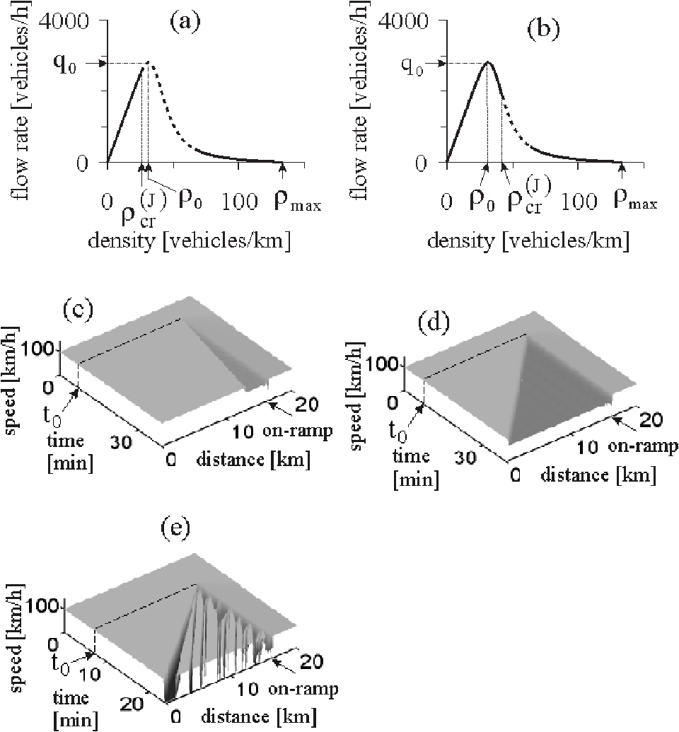
There are two possibilities for the arrangement of the point of this instability on the fundamental diagram in the OV model and other models in the context of the fundamental diagram approach:
(i) The point lies left of the maximum point of the fundamental diagram , i.e., on the branch of the diagram with a positive slope (figure 13 (a)):
| (73) |
(ii) The point lies right of the maximum point of the fundamental diagram , i.e., on the branch of the diagram with a negative slope (figure 13 (b)):
| (74) |
Note that in both cases (i) and (ii) all states on the fundamental diagram, in which the density satisfies the condition
| (75) |
where is the density in the wide moving jam outflow associated with the flow rate , are metastable states with respect to moving jam emergence [44]. The case (i) has intensively been considered in the literature [3, 4, 5, 6] and criticized in Sect. 3.3.2 of the book [7].

In the case (ii) (figure 13 (b)), the flow rate in free flow downstream of an on-ramp bottleneck cannot exceed the maximum flow rate on the fundamental diagram . If is a given large enough value and the flow rate begins to increase, then a localized perturbation as that in the ATD- and SA-models (Sects. 4.1 and 5.1) appears at the bottleneck (figures 14 (a) and (b)). The minimum speed within the time-averaged (deterministic) perturbation on the main road decreases when increases (points 1–3 in figure 14 (c)). In the OV-model, when increases, the location of the minimum speed within the deterministic perturbation on the main road exhibits firstly a slight shift downstream and then upstream within the merging region of the on-ramp (figure 14 (a, b)). For this reason, the flow rate on the main road at the location of the minimum speed within the deterministic perturbation on the main road firstly slightly increases and then decreases (points 1–3 in figure 14 (d)), whereas the flow rate on the main road upstream of the on-ramp merging region is equal to (points 1–3 in figure 14 (e)). When increases beginning from zero, the flow rate downstream of the bottleneck increases beginning from (points 1–3 in figures 14 (f) and (g)).
At a given large enough flow rate this growth of the local perturbation in free flow at the bottleneck with has a limit. This limit is reached when the flow rate reaches some critical value at which the flow rate is equal to the maximum flow rate on the fundamental diagram:
| (76) |
When the flow rate increases further, i.e.,
| (77) |
then the upstream front of the initial perturbation, which is motionless at the condition (curve II in figure 14 (h)), begins to move upstream of the bottleneck, i.e., a wave of lower speed and greater density propagating upstream appears (spatial speed distributions related to the times – in figure 14 (h)). As a result, a dense flow associated with the branch of the diagram with a negative slope occurs upstream of the bottleneck (figures 13 (c) and (d) and points 4–6 in figures 14 (c)–(e)). At the critical point (76), the derivative of the minimum average speed on the main road on the flow rate is discontinuous, whereas this speed is a continuous decreasing function of (figure 14 (c)). The greater the flow rate , specifically, the greater (77), the greater absolute velocity of the wave of dense flow propagation (figures 13 (c) and (d)). In addition, the flow rate downstream of the bottleneck, which is equal to under the condition (76), remains approximately to be equal to , when increases (points 4–6 in figures 14 (f) and (g)).
It must be noted that the above mentioned behaviour of the upstream front of the perturbation at the bottleneck in the OV model (71), (74) is qualitatively different from those for the upstream front of the perturbation at the bottleneck in the ATD- and SA-models. In the latter case, when the flow rate reaches the critical value for an FS transition, a wave of synchronized flow occurs abruptly and propagates upstream with a finite velocity. This is associated with a first-order FS transition. In contrast, in the OV-model there is no discontinuous change in the velocity when due to an increase in the condition (77) is satisfied: increases continuously beginning from zero, when first reaches and then exceeds the critical flow rate associated with the condition (76). Specifically, we find that if , then . Thus, in the OV-model there is no first-order phase transition from free flow to dense flow.
The widening dense flow upstream of the bottleneck (figures 13 (c) and (d) and 14 (h)) can exist only, when the density in the dense flow satisfies the condition
| (78) |
This is because at the density the dense flow loses its stability against wide moving jam emergence (point 7 and dotted down-arrow in figure 14 (c)). However, dynamic waves that emerge due to vehicle merging at the bottleneck propagate through the dense flow. For this reason, in numerical simulations this moving jam emergence occurs already at the density (point 6 and solid down-arrow in figure 14 (c)).
The congested patterns in figures 13 (d) and (e) at the first glance resemble a widening SP and an GP, respectively. Indeed, in both cases a dense flow occurs upstream of the bottleneck whose downstream front is fixed at the bottleneck. Thus, this dense flow should satisfy the macroscopic spatiotemporal objective criteria for the synchronized flow phase (Sect. 1). This conclusion is, however, incorrect. To explain this, note that in empirical observations application of the objective criteria, which define the traffic phases in congested traffic, leads to clear distinction of the synchronized flow phase. This synchronized flow exhibits the following fundamental empirical feature: An FS transition leading to synchronized flow emergence is a first-order phase transition. In contrast, in a traffic flow model an application of the objective criteria does not guarantee that dense flow occurrence in free flow is associated with a first-order phase transition, which is one of the requirements for the synchronized flow phase.
This conclusion concerns the OV model (71), (74) (figure 13 (b)) as well as other models in the context of the fundamental diagram approach under condition (74). Whereas for the SA-model there is a Z-shaped speed–flow characteristic associated with a first-order FS transition in free flow at the bottleneck (figures 6 (c)–(e)), for the OV model the on-ramp flow rate dependence of the speed at the bottleneck is a monotonous decreasing function (figure 14 (c)): There is no first-order phase transition, when a dense flow related to the fundamental diagram with a negative slope is formed upstream of the bottleneck. Thus, the dense traffic flow in the case of the OV model and other models in the context of the fundamental diagram approach under condition (74) does not exhibit the important empirical feature of synchronized flow and, therefore, the dense flow is not associated with the synchronized flow phase.
There are also traffic flow models in the context of the fundamental diagram approach, in which there is no instability of steady model states on the fundamental diagram regardless of the vehicle density. Examples of this model class are as follows: (i) An OV model (71) in which the sensitivity is great enough regardless of and . (ii) The Nagel-Schreckenberg cellular automata model in the deterministic model limit, i.e., when probability of model fluctuations in this model is equal zero () [46]. (iii) The Lighthill-Whitham-Richards model [47] and the associated cell-transmission models [48]. In this model class, traffic patterns at a freeway bottleneck are qualitatively similar as those found in the OV model (71), (74) at the density considerably smaller than the critical density (the patterns associated with points 1–5 in figures 14 (c)–(g)). These common model features are as follows: 1) the local perturbation at the bottlenecks at (figures 14 (a) and (b)); 2) widening dense flow upstream of the bottleneck at (figures 13(c) and (d) and 14 (h)); 3) there is no discontinuous change in speed (no speed breakdown) at the bottleneck when widening dense flow occurs; 4) with an increase in traffic demand at , the upstream front velocity of widening dense flow increases continuously beginning from zero. Thus, in this model class, there is no first-order FS transition observed during the onset of congestion at the bottleneck, i.e., this dense flow has no relation to real freeway traffic.
6.3 Conclusions
(i) Two different deterministic microscopic traffic flow model classes in the context of three-phase traffic theory, the ATD- and SA-models, have been introduced in the article.
(ii) The ATD- and SA-models reproduce important empirical spatiotemporal features of phase transitions in traffic flow and congested traffic patterns.
(iii) In contrast with all other known deterministic microscopic traffic flow models, in the ATD- and SA-models vehicles moving in free flow and vehicles moving in synchronized flow exhibit qualitatively different dynamic behaviour. This is a result of the introduction of two separated regions of steady state model solutions for free flow and synchronized flow in the ATD- and SA-models as well as different dynamic rules of vehicle motion in free flow and synchronized flow implemented in the models.
(iv) As in empirical observations, there is a first-order phase transition in the ATD- and SA-models from free flow to synchronized flow that explained the onset of congestion at bottlenecks in these models.
(v) The nature of the onset of congestion as a first-order FS transition in free flow at the bottleneck, which the ATD- and SA-models show, is also associated with metastability of free flow at the bottleneck against external short-time disturbances in this flow in a neighbourhood of the bottleneck. As a result, there is multiple congested pattern emergence in an initial free flow at the bottleneck in the ATD- and SA-models: Depending on an amplitude (or duration) of an external disturbance, one of the SPs or else an GP can be induced in free flow at the bottleneck at the same chosen model parameters.
(vi) In accordance with empirical results, in the ATD- and SA-models moving jams can emerge spontaneously in synchronized flow only, i.e., as a result of FSJ transitions.
(vii) In addition to the above common behaviour of the ATD- and SA-models, these models exhibit also some qualitatively different features. This is because in the ATD-model synchronized flow model steady states are related to a 2D-region in the flow–density plane, whereas synchronized flow model steady states in the SA-models belong to an 1D-region (a curve) in the flow–density plane. In particular, the following differences of model features have been found:
(1) The ATD-model can show all types of spatiotemporal congested patterns at an on-ramp bottleneck observed in empirical observations.
(2) In contrast, SA-models cannot show LSPs associated with empirical results as well as some of empirical features of synchronized flow between wide moving jams within GPs.
(viii) Models in the context of the fundamental diagram approach reviewed in [1, 2, 3, 4, 5, 6] cannot explain the onset of congestion in free flow, which in empirical observations is associated with a first-order FS transition. Depending on the model type and model parameters, in these models either wide moving jam emergence is responsible for the onset of congestion at an on-ramp bottleneck rather than an empirically observed FS transition or a widening dense traffic flow occurs upstream of the bottleneck when the density in free flow at the bottleneck exceeds the density associated with the maximum point on the fundamental diagram. In the latter case, in contrast with empirical observations there is no first-order phase transition from an initial free flow to this dense flow at the bottleneck: The dense flow results from non-homogeneity of a freeway in a neighbourhood of the bottleneck. Thus, these models cannot show a first-order FS transition observed during the onset of congestion at the bottleneck in real freeway traffic, i.e., this dense flow has no relation to real freeway traffic. Indeed, the first-order FS transition is a fundamental empirical feature of the onset of congestion in free flow with the subsequent synchronized flow phase emergence at the bottleneck.
Appendix A
To derive formula (23) [45], let us consider a solution of (19) when it is an equality:
| (79) |
From (19), (79), it can be seen that if , then the safe speed ; if in contrast , then the speed . In particular, this ensures collision less vehicle motion. To simplify the formula (79), let us replace the space gap in denominator of (79) by the value . This reduces the safe speed at , therefore, the safety condition (19) remains to be valid. Then from formula (79), we get
| (80) |
To provide more comfortable vehicle deceleration, an anticipated gap is used in formula (80) rather than the gap . As a result, (80) takes the form
| (81) |
Substituting (81) into (18), we find formula (23) with coefficiens (24), (25).
Note that we have also tested another formulation for the safe speed in the ATD-model when the speed in (18) is given by formula (79). Simulations of the ATD-model show that both formulations (23) and (79) ensure collision less vehicle motion at an appropriate choice of model parameters and lead to qualitatively the same features of phase transitions and congested patterns.
Appendix B
In this Appendix, two further variants of the SA-models are presented. In the first of these variants, the formula (3.2) reads as follows
where , , are given by (53)–(57). In this SA-model, steady states of free flow (the curve in figure 2 (e)) correspond to the condition (59), averaged steady states of synchronized flow are related to a line given by the condition
| (86) |
steady states for a wide moving jam are associated with the condition (63) (figure 2 (e)).
In another variant of SA-model, formula (3.2) reads as follows
In (B), is the maximum space gap in synchronized flow; , , are given by (53) in which is taken from (56),
| (92) |
| (93) |
where the sensitivity
is a sensitivity, is given by (57). A function in (B) is taken as follows
| (97) |
where the function at , is a sensitivity that in a general case can be different from the sensitivity in free flow.
In the SA-model (B)–(B), steady states of free flow (the curve in figure 2 (f)) are associated with the condition (59), averaged steady states of synchronized flow are related to a line given by the condition
| (98) |
where , and steady states for a wide moving jam are found from the condition (63) (figure 2 (f)).
In contrast with the other SA-models, the SA-model (B)–(B) has a limited density range of steady states between steady states for free flow and synchronized flow, which are found from the condition
| (99) |
Eq. (99) yields the following condition for these steady states in the flow–density plane (curve in figure 2 (f))
| (100) |
where the density at the maximum point for free flow is not greater than the density associated with the maximum point on the curve (figure 2 (f)). To simulate a first-order FS transition, the steady state model solutions (100) should be unstable against infinitesimal non-homogeneous perturbations. This requirement to the SA-model (B)–(B) is easy satisfied through an appropriated choice of the function and the sensitivities , , . In this case, numerical simulations of the SA-model (B)–(B) made show that this model exhibits FSJ transitions in accordance with empirical results (we used the following parameters for the SA-model (B)–(B): with 14 m/s, 21 m, 7 m; 24 m; ; ; ; is taken from Table 1 with , 9 m/s, 0.05; other parameters are the same as those in the SA-model (48)–(57)).
References
- [1] N.H. Gartner, C.J. Messer, A. Rathi (eds.). Special Report 165: Revised Monograph on Traffic Flow Theory (Transportation Research Board, Washington, D.C. 1997)
- [2] D.E. Wolf. Physica A 263, 438 (1999)
- [3] D. Chowdhury, L. Santen, A. Schadschneider. Physics Reports 329, 199 (2000)
- [4] D. Helbing. Rev. Mod. Phys. 73, 1067–1141 (2001)
- [5] T. Nagatani. Rep. Prog. Phys. 65, 1331–1386 (2002)
- [6] K. Nagel, P. Wagner, R. Woesler. Operation Res. 51, 681–716 (2003)
- [7] B.S. Kerner. The Physics of Traffic (Springer, Berlin, New York 2004).
- [8] J.-B. Lesort (editor). Transportation and Traffic Theory, Proceedings of the 13th International Symposium on Transportation and Traffic Theory (Elsevier Science Ltd, Oxford 1996)
- [9] A. Ceder (editor). Transportation and Traffic Theory, Proceedings of the 14th International Symposium on Transportation and Traffic Theory (Elsevier Science Ltd, Oxford 1999)
- [10] M.A.P. Taylor (editor). Transportation and Traffic Theory in the 21st Century, Proceedings of the 15th International Symposium on Transportation and Traffic Theory (Elsevier Science Ltd, Amsterdam 2002)
- [11] D.E. Wolf, M. Schreckenberg, A. Bachem (editors). Traffic and Granular Flow, Proceedings of the International Workshop on Traffic and Granular Flow, October 1995 (World Scientific, Singapore 1995)
- [12] M. Schreckenberg, D.E. Wolf (editors). Traffic and Granular Flow’ 97, Proceedings of the International Workshop on Traffic and Granular Flow, October 1997 (Springer, Singapore 1998)
- [13] D. Helbing, H.J. Herrmann, M. Schreckenberg, D.E. Wolf (editors). Traffic and Granular Flow’ 99, Proceedings of the International Workshop on Traffic and Granular Flow, October 1999, (Springer, Heidelberg 2000)
- [14] M. Fukui, Y. Sugiyama, M. Schreckenberg, D.E. Wolf (editors). Traffic and Granular Flow’ 01, Proceedings of the International Workshop on Traffic and Granular Flow, October 2001, (Springer, Heidelberg 2003)
- [15] S.P. Hoogendoorn, S. Luding, P.H.L. Bovy, M. Schreckenberg, D.E. Wolf (editors). Traffic and Granular Flow’ 03, Proceedings of the International Workshop on Traffic and Granular Flow, October 2003, (Springer, Heidelberg 2005)
- [16] H.J. Payne. In: Mathematical Models of Public Systems, edited by G.A. Bekey, Vol. 1 (Simulation Council, La Jolla 1971); Transportation Research Record 772, 68 (1979)
- [17] R. Kühne: In: Highway Capacity and Level of Service, edited by U. Brannolte (A.A. Balkema, Rotterdam 1991) pp. 211
- [18] B.S. Kerner, P. Konhäuser. Phys. Rev. E 48 2335–2338 (1993)
- [19] A. Klar, R. Kühne, R. Wegener Surv. Math. Ind., 6, 215–239 (1996).
- [20] N. Bellomo, M. Delitala, V. Coscia. Math. Models Meth. Appl. Sci. 12, 1801–1844 (2002).
- [21] S. Darbha, K.R. Rajagopal. Systems and Control Letters 43, 387-401 (2001).
- [22] 4. S. Darbha, K.R. Rajagopal. Mathematical Problems in Engineering 7, 379-392 (2001).
- [23] R. Herman, E.W. Montroll, R.B. Potts, R.W. Rothery. Operations Res. 7, 86–106 (1959).
- [24] D. C. Gazis, R. Herman, and R. W. Rothery, Operations Res. 9, 545–567 (1961).
- [25] T. Nagatani and K. Nakanishi, Phys. Rev. E 57, 6415 (1998).
- [26] I. Lubashevsky, P. Wagner, R. Mahnke, European Phys. J. B 32, 243–247 (2003).
- [27] G.F. Newell, Operations Res. 9, 209 (1961).
- [28] G.B. Whitham, Proc. R. Soc. London A 428, 49 (1990).
- [29] M. Bando, K. Hasebe, A. Nakayama, A. Shibata, Y. Sugiyama, Jpn. J. Appl. Math. 11, 203 (1994); Phys. Rev. E 51, 1035–1042 (1995).
- [30] M. Treiber, D. Helbing, e-print, cond-mat/9901239 (1999).
- [31] M. Treiber, A. Hennecke, D. Helbing, Phys. Rev. E 62, 1805–1824 (2000).
- [32] B.S. Kerner, H. Rehborn. Phys. Rev. Lett. 79, 4030 (1997).
- [33] B. S. Kerner, Phys. Rev. Lett. 81, 3797 (1998).
- [34] B. S. Kerner, Phys. Rev. E 65, 046138 (2002).
- [35] B.S. Kerner, S.L. Klenov: J. Phys. A: Math. Gen. 35, L31 (2002)
- [36] B.S. Kerner, S.L. Klenov, D.E. Wolf, J. Phys. A: Math. Gen. 35 9971–10013 (2002).
- [37] B.S. Kerner, S.L. Klenov, Phys. Rev. 68 036130 (2003)
- [38] B.S. Kerner, S.L. Klenov: J. Phys. A: Math. Gen. 37 8753–8788 (2004).
- [39] B.S. Kerner, S.L. Klenov, H. Hiller: physics/0507094 (2005). E-print in http://arxiv.org/abs/physics/0507094.
- [40] L.C. Davis: Phys. Rev. E 69 016108 (2004).
- [41] H.K. Lee, R. Barlović, M. Schreckenberg, D. Kim: Phys. Rev. Let. 92, 238702 (2004).
- [42] R. Jiang, Q.S. Wu: J. Phys. A: Math. Gen. 37, 8197–8213 (2004).
- [43] P.G. Gipps: Trans. Res. B. 15, 105–111 (1981); 20, 403–414 (1986).
- [44] B.S. Kerner, P. Konhäuser: Phys. Rev. E 50, 54–83 (1994).
- [45] B.S. Kerner, S.L. Klenov: physics/0507120 (2005), E-print in http://arxiv.org/abs/physics/0507120.
- [46] Nagel K and Schreckenberg M 1992 J Phys. (France) I 2 2221
- [47] Lighthill M J and Whitham G B 1955 Proc. R. Soc. A 229 317 Richards P I 1956 Operations Res. 4 42
- [48] Daganzo C 1999 In [9] 81-104