Turbulent Friction in Rough Pipes and the Energy
Spectrum of the Phenomenological Theory

Turbulence is the unrest that spontaneously takes over a streamline flow adjacent to a wall or obstacle when the flow is made sufficiently fast. Although most of the flows that surround us in everyday life and in nature are turbulent flows over rough walls, these flows have remained amongst the least understood phenomena of classical physics jimenez; antonia. Thus, one of the weightier experimental studies of turbulent flows on rough walls, and the most useful in common applications, is yet to be explained theoretically 70 years after its publication. In that study niku, Nikuradse elucidated how the friction coefficient between the wall of a pipe and the turbulent flow inside depends on the Reynolds number of the flow and the roughness of the wall. The friction coefficient, $f$, is a measure of the shear stress (or shear force per unit area) that the turbulent flow exerts on the wall of a pipe; it is customarily expressed in dimensionless form as $f=\tau/\rho V^{2}$, where $\rho$ is the density of the liquid that flows in the pipe and $V$ the mean velocity of the flow. The Reynolds number is defined as ${\rm Re}=VR/\nu$, where $R$ is the radius of the pipe and $\nu$ the kinematic viscosity of the liquid. Last, the roughness is defined as the ratio $r/R$ between the size $r$ of the roughness elements (sand grains in the case of Nikuradse’s experiments) that line the wall of the pipe and the radius of the pipe.

Nikuradse presented his data in the form of six curves, the log-log plots of $f$ versus Re for six values of the roughness niku. These curves are shown in Fig. 1. At the onset of turbulence hof, at a Re of about 3,000, all six curves rise united in a single bundle. At a Re of about 3,500, the bundle bends downward to form a marked hump and then it plunges in accord with Blasius’s empirical scaling prandtl, $f\sim{\rm Re}^{-1/4}$, as one by one in order of decreasing roughness the curves start to careen away from the bundle. After leaving the bundle, which continues to plunge, each curve sets out to trace a belly belly as it steers farther from the bundle with increasing Re, then flexes towards a terminal, constant value of $f$ that is in keeping with Strickler’s empirical scaling strickler, $f\sim(r/R)^{1/3}$. For seventy years now, our understanding of these curves has been aided by little beyond a pictorial narrative of roughness elements being progressively exposed to the turbulent flow as Re increases chow.

In our theoretical work, we adopt the phenomenological imagery of “turbulent eddies” rich; kolmo; frisch and use the spectrum of turbulent energy pope at a lengthscale $\sigma$, $E(\sigma)$, to determine the velocity of the eddies of size $s$, $u_{s}$, in the form $u_{s}^{2}=\int_{0}^{s}E(\sigma)\sigma^{-2}d\sigma$, where $E(\sigma)=A\,\varepsilon^{2/3}\sigma^{5/3}c_{d}(\eta/\sigma)c_{e}(\sigma/R)$. Here $A$ is a dimensionless constant, $\varepsilon$ is the turbulent power per unit mass, $\eta=\nu^{3/4}\varepsilon^{-1/4}$ is the viscous lengthscale, $R$ is the largest lengthscale in the flow, $A\,\varepsilon^{2/3}\sigma^{5/3}$ is the Kolmogórov spectrum (which is valid in the inertial range, $\eta\ll\sigma\ll R$), and $c_{d}$ and $c_{e}$ are dimensionless corrections for the dissipative range and the energetic range, respectively. For $c_{d}$ we adopt an exponential form, $c_{d}(\eta/\sigma)=\exp(-\beta\eta/\sigma)$ (which gives $c_{d}\approx 1$ except in the dissipative range, where $\sigma\approx\eta$), and for $c_{e}$ the form proposed by von Kármán, $c_{e}(\sigma/R)=(1+\gamma(\sigma/R)^{2})^{-17/6}$ (which gives $c_{e}\approx 1$ except in the energetic range, where $\sigma\approx R$), where $\beta$ and $\gamma$ are dimensionless constants pope. To obtain expressions for $u_{s}$ and $\eta$ in terms of Re, $r/R$, and $V$, we invoke the usual scalings tl, $\varepsilon=\kappa_{\varepsilon}\,u_{R}^{3}/R$ (Taylor’s scaling taylor, where $u_{R}$ is the characteristic velocity of the largest eddies and $\kappa_{\varepsilon}$ a dimensionless constant) and $u_{R}=\kappa_{u}V$ (where $\kappa_{u}$ is a dimensionless constant). Then, we can write $\eta=bR\,{\rm Re}^{-3/4}$, where $b\equiv(\kappa_{\varepsilon}\kappa_{u}^{3})^{-1/4}$, and (after changing the integration variable to $x\equiv\sigma/R$) $u_{s}^{2}=A\,\kappa_{\varepsilon}^{2/3}u_{R}^{2}\int_{0}^{s/R}x^{-1/3}c_{d}(b\,{\rm Re}^{-3/4}/x)c_{e}(x)dx$. For $s\ll R$ we can set $c_{e}=1$, compute the integral, and let ${\rm Re}\to\infty$ to obtain $u_{s}^{2}=(3/2)A\,\kappa_{\varepsilon}^{2/3}u_{R}^{2}\,(s/R)^{2/3}$, or $u_{s}^{2}\sim u_{R}^{2}(s/R)^{2/3}$, a well-known result of the phenomenological theory. Further, for consistency with Taylor’s scaling we must have $A\,\kappa_{\varepsilon}^{2/3}=2/3$ (so that $u_{s}=u_{R}$ for $s=R$) and therefore $u_{s}^{2}=\kappa_{u}^{2}\,V^{2}(2/3)\int_{0}^{s/R}x^{-1/3}c_{d}(b\,{\rm Re}^{-3/4}/x)c_{e}(x)dx$.

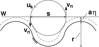
We now seek to derive an expression for $\tau$, the shear stress on the wall of the pipe. We assume a viscous layer of constant thickness $a\eta$, where $a$ is a dimensionless constant, and call $W$ a wetted surface parallel to the peaks of the viscous layer (Fig. 2). Then, $\tau$ is effected by momentum transfer across $W$. Above $W$, the velocity of the flow scales with $V$, and the fluid carries a high horizontal momentum per unit volume ($\sim\rho V$). Below $W$, the velocity of the flow is negligible, and the fluid carries a negligible horizontal momentum per unit volume. Now consider an eddy that straddles the wetted surface $W$. This eddy transfers fluid of high horizontal momentum downwards across $W$, and fluid of negligible horizontal momentum upwards across $W$. The net rate of transfer of momentum across $W$ is set by the velocity normal to $W$, which velocity is provided by the eddy. Therefore, if $v_{n}$ denotes the velocity normal to $W$ provided by the dominant eddy that straddles $W$, then the shear stress effected by momentum transfer across $W$ scales in the form $\tau\sim\rho\,Vv_{n}$.

In order to identify the dominant eddy that straddles $W$, let us denote by $s=r+a\eta$ the size of the largest eddy that fits the coves between successive roughness elements. Eddies much larger than $s$ can provide only a negligible velocity normal to $W$. (This observation is purely a matter of geometry.) On the other hand, eddies smaller than $s$ can provide a sizable velocity normal to $W$. Nevertheless, if these eddies are much smaller than $s$, their velocities are overshadowed by the velocity of the eddy of size $s$. Thus, $v_{n}$ scales with $u_{s}$, which is the velocity of the eddy of size $s$, and the dominant eddy is the largest eddy that fits the coves between successive roughness elements. We conclude that $\tau\sim\rho\,Vu_{s}$, or $\tau=\kappa_{\tau}\rho\,Vu_{s}$ (where $\kappa_{\tau}$ is a dimensionless constant of order 1), and therefore $f=\kappa_{\tau}u_{s}/V$ or

where $K\equiv\kappa_{\tau}\kappa_{u}\sqrt{2/3}$, $s/R=r/R+ab\,{\rm Re}^{-3/4}$, and $b\equiv(\kappa_{\varepsilon}\kappa_{u}^{3})^{-1/4}$. Equation (1) gives $f$ as an explicit function of the Reynolds number Re and the roughness $r/R$.

To evaluate computationally the integral of (1), we set $\beta=2.1$, $\gamma=6.783$ (the values given in pope), $a=5$ ($5\eta$ being a common estimation of the thickness of the viscous layer), $\kappa_{\varepsilon}=5/4$ (a value that follows from Kolmogórov’s four-fifth law ff), $\kappa_{u}=0.036$ ($0.036\pm 0.005$ being the value measured in pipe flow by Antonia and Pearson ap), $b\equiv(\kappa_{\varepsilon}\kappa_{u}^{3})^{-1/4}=11.4$, and treat $\kappa_{\tau}$ as a free parameter (albeit a parameter constrained by theory to be of order 1). With $\kappa_{\tau}=0.5$ (and therefore $K=0.015$), (1) gives the plots of Fig. 3. (Note that a different value of $\kappa_{\tau}$ would give the same plots except for a vertical translation.) These plots show that (1) is in excellent qualitative agreement with Nikuradse’s data, right from the onset of turbulence, including the hump and, for relatively low roughness, the bellies. These plots remain qualitatively the same even if the value of any of the parameters is changed widely. In particular, there is always a hump and there are always bellies: these are robust features closely connected with the overall form of the spectrum of turbulent energy. The connections will become apparent after the discussion that follows.

To help interpreting our results, we compute $f$ without including the correction for the energetic range—that is, setting $\gamma=0$. In this case, the integral of (1) may be evaluated analytically, with the result

where $F(y)=y^{2/3}\Gamma_{-2/3}(y)$, $\Gamma_{-2/3}$ is the gamma function of order $-2/3$, and $y=\beta\eta/s=\beta b\,{\rm Re}^{-3/4}(r/R+ab\,{\rm Re}^{-3/4})^{-1}$. With the same values of $\kappa_{\tau}$, $\kappa_{u}$, $a$, $b$, and $\beta$ as before, (2) gives the solid-line plots in the inset of Fig. 3. The hump is no more. We conclude that the hump relates to the energetic range. Further, with the exception of the hump at relatively low Re, the plots of (1) coincide with the plots of (2); thus, we can study (2) to reach conclusions about (1) at intermediate and high Re. For example, (2) gives $f\sim(r/R)^{1/3}$ for $r\gg a\eta$ and $f\sim{\rm Re}^{-1/4}$ for $r\ll a\eta$. It follows that both (2) and (1) give a gradual transition between the empirical scalings of Blasius and Strickler gb, in accord with Nikuradse’s data.

If we set $\beta=0$ in addition to $\gamma=0$, (2) simplifies to $f=\kappa_{\tau}\kappa_{u}\,(r/R+ab\,{\rm Re}^{-3/4})^{1/3}$. With the same values of $\kappa_{\tau}$, $\kappa_{u}$, $a$, and $b$ as before, this expression gives the dashed-line plots in the inset of Fig. 3. Now the bellies are no more. We conclude that the bellies relate to the dissipative range. The dissipation depresses the values of $f$ at relatively low and intermediate Re, leading to the formation of the bellies of Nikuradse’s data.

We are ready to explain the unfolding of Nikuradse’s data in terms of the varying habits of momentum transfer with increasing Re (Fig. 4). At relatively low Re, the inertial range is immature, and the momentum transfer is dominated by eddies in the energetic range, whose velocity scales with $V$, and therefore with Re. Consequently, an increase in Re leads to a more vigorous momentum transfer—and to an increase in $f$. This effect explains the rising part of the hump. At higher Re, the momentum transfer is dominated by eddies of size $s\approx a\eta\gg r$. Since $\eta\sim{\rm Re}^{-3/4}$, with increasing Re the momentum transfer is effected by ever smaller (and slower) eddies, and $f$ lessens as Re continues to increase. This effect explains the plunging part of the hump—the part governed by Blasius’s scaling. At intermediate Re, $s=r+a\eta$ with $r\approx a\eta$. Due to the decrease in $\eta$, $s$ continues to lessen as Re continues to increase, but at a lower rate than before, when it was $s\approx a\eta\gg r$. Thus, the curve associated with $r$ deviates from Blasius’s scaling and starts to trace a belly. As $\eta$ continues to decrease, the dominant eddies become decidedly larger than the smaller eddies in the inertial range, which is well established now, and any lingering dissipation at lengthscales larger than $s$ must cease. This effect explains the rising part of the belly. Last, at high Re, $s\approx r\gg a\eta$. As Re increases further, $\eta$ lessens and new, smaller eddies populate the flow and become jumbled with the preexisting eddies. Yet the momentum transfer continues to be dominated by eddies of size $r$, and $f$ remains invariant. This effect explains Nikuradse’s data at high Re, where $f$ is governed by Strickler’s scaling.

We have predicated equation (1), on the assumption that the turbulent eddies are governed by the phenomenological theory of turbulence. The theory was originally derived for isotropic and homogeneous flows, but recent research aniso suggests that it applies to much more general flows as well. Our results indicate that even where the flow is anisotropic and inhomogeneous—as is the case in the vicinity of a wall—the theory gives an approximate solution that embodies the essential structure of the complete solution (including the correct scalings of Blasius and Strickler) and is in detailed qualitative agreement with the observed phenomenology. Remarkably, the qualitative agreement holds starting at the very onset of turbulence, in accord with experimental evidence that “in pipes, turbulence sets in suddenly and fully, without intermediate states and without a clear stability boundary” hof. The deficiencies in quantitative agreement point to a need for corrections to account for the effect of the roughness elements on the dissipative range as well as for the effect of the overall geometry on the energetic range.

In conclusion, to a good approximation the eddies in a pipe are governed by the spectrum of turbulent energy of the phenomenological theory. The size of the eddies that dominate the momentum transfer close to the wall is set by a combination of the size of the roughness elements and the viscous lengthscale. As a result, the dependence of the turbulent friction on the roughness and the Reynolds number is a direct manifestation of the distribution of turbulent energy given by the phenomenological theory. This close relation between the turbulent friction and the phenomenological theory ng may be summarized in the following observation: the similarity exponents of Blasius and Strickler are but recast forms of the exponent $5/3$ of the Kolmogórov spectrum.