Workload characterization and modelling
August 11, 2026
Workload analysis of a cluster
in a Grid environment
Thanks: This work was supported by EGEE.
Abstract
With Grids, we are able to share computing resources and to provide for scientific communities a global transparent access to local facilities. In such an environment the problems of fair resource sharing and best usage arise. In this paper, the analysis of the LPC cluster usage (Clermont-Ferrand, France) in the EGEE Grid environment is done, and from the results a model for job arrival is proposed.
1 Introduction
Analysis of a cluster workload is essential to understand better user behavior and how resources are used [1]. We are interested to model and simulate the usage of a Grid cluster node in order to compare different scheduling policies and to find the best suited one for our needs.
The Grid gives new ways to share resources between sites, both as computing and storage resources. Grid defines a global architecture for distributed scheduling and resource management [2] that enable resources scaling. We would like to understand better such a system so that a model can be defined. With such a model, simulation may be done and a quality of service and fairness could then be proposed to the different users and groups.
Briefly, we have some groups of users that each submit jobs to a group of clusters. These jobs are placed inside a waiting queue on some clusters before being scheduled and then processed. Each group of users have their own need and their own strategy to job submittal. We wish:
- 1.
to have good metrics that describes the group and user usage of the site.
- 2.
to model the global behavior (average job waiting time, average waiting queue length, system utilization, etc.) in order to know what is the influence of each parameter and to avoid site saturation.
- 3.
to simulate jobs arrivals and characteristics to test and compare different scheduling strategies. The goal is to maximize system utilization and to provide fairness between site users to avoid job starvation.
As parallel scheduling for machines is a hard problem [3, 4], heuristics are used [5, 6]. Moreover we have no exact value about the duration of jobs, making the problem difficult. We need a good model to be able to compare different scheduling strategies. We believe that being able to characterize users and groups behavior we could better design scheduling strategies that promote fairness and maintain a good throughput. From this paper some metrics are revealed, from the job submittal protocol a detailed arrival model for single user and group is proposed and scheduling problems are discussed. We then suggest a new design based on our observation and show relationship between fairness issue and system utilization as a flow problem.
Our cluster usage in the EGEE (Enabling Grids for E-science in Europe) Grid is presented in section 2, the Grid middleware used is described. Corresponding scheduling scheme is shown in section 3. Then the workload of the LPC (Laboratoire de Physique Corpusculaire) computing resource, is presented (section 4) and the logs are analyzed statistically. A model is then proposed in section 5 that describes the job arrival rate to this cluster. Simulation and validation are done in section 6 with comparison with related works in section 7. Results are discussed in section 8. Section 9 concludes this paper.
2 Environment
2.1 Local situation
The EGEE node at LPC Clermont-Ferrand is a Linux cluster made of 140 dual 3.0 GHz CPUs with 1 GB of RAM and managed by 2 servers with the LCG (LHC Computing Grid Project) middleware. We are currently using MAUI as our cluster scheduler [7, 8]. It is shared with the regional Grid INSTRUIRE (http://www.instruire.org). Our LPC Cluster role in EGEE is to be used mostly by Biomedical users** * Our cluster represented 75% of all the Biomed Virtual Organization (VO) jobs in 2004. located in Europe and by High Energy Physics Communities. Biomedical research is one core application of the EGEE project. The approach is to apply the computing methods and tools developed in high energy physics for biomedical applications. Our team has been involved in international research group focused on deploying biomedical applications in a Grid environment.
One pilot application is GATE which is based on the Monte Carlo GEANT4 [9] toolkit developed by the high energy physics community. Radiotherapy and brachytherapy use ionizing radiations to treat cancer. Before each treatment, physicians and physicists plan the treatment using analytical treatment planning systems and medical images data of the tumor. By using the Grid environment provided by the EGEE project, we will be able to reduce the computing time of Monte Carlo simulations in order to provide a reasonable time consuming tool for specific cancer treatment requiring Monte-Carlo accuracy.
Another group is Dteam, this group is partly responsible of sending tests and monitoring jobs to our site. Total CPU time used by this group is small relatively to the other one, but the jobs sent are important for the site monitoring. There are also groups using the cluster from the LHC experiments at CERN (http://www.cern.ch). There are different kind of jobs for a given group. For example, Data Analysis requires a lot of I/O whereas Monte-Carlo Simulation needs few I/O.
2.2 EGEE Grid technology
In Grid world, resources are controlled by their owners. For instance different kind of scheduling policies could be used for each site. A Grid resource center provides to the Grid computing and/or storage resources and also services that allow jobs to be submitted by guests users, security services, monitoring tools, storage facility and software management. The main issue of submitting a job to a remote site is to provide some warranty of security and correct execution. In fact the middleware automatically resubmits job when there is a problem with one site. Security and authentication are also provided as Grid services.
The Grid principle is to allow user a worldwide transparent access to computing and storage resources. In the case of EGEE, this access is aimed to be transparent by using LCG middleware built on top of the Globus Toolkit [10]. Middleware acts as a layer of software that provides homogeneous access to different Grid resource centers.
2.3 LCG Middleware
LCG is organized into Virtual Organizations (VOs): dynamic collections of individuals and institutions sharing resources in a flexible, secure and coordinated manner. Resource sharing is facilitated and controlled by a set of services that allow resources to be discovered, accessed, allocated, monitored and accounted for, regardless of their physical location. Since these services provide a layer between physical resources and applications, they are often referred to as Grid Middleware [11].
Bag of task applications are parallel applications composed of independent jobs. No communications are required between running jobs. Since jobs from a same task may execute on different sites communications between jobs are avoided. In this context, users submit their jobs to the Grid one by one through the middleware. Our cluster receives jobs only from the Grid. This means that each job requests for one and only one processor. Users could directly specify the execution site or let a Grid service choose the best destination for them. Users give only a rough estimation of the maximum job running time. In general this estimated time is overestimated and very imprecise [12]. Instead of speaking about an estimated time, it could be better to speak about an upper bound for job duration, so this value provided by users is more a precision value. The bigger the value is the more imprecise the value of the actual runtime could be.
Figure 1 shows the scenario of a job submittal. In this figure rounded boxes are grid services and ellipses are the different jobs states. As there is no communications between jobs, jobs could run independently on multiple clusters. Instead of communicating between job execution, jobs write output files to Storage Elements (SE) of the Grid. Small output files could also be sent to the UI. Replica Location Service (RLS) is a Grid service that allow location of replicated data. Other jobs may read and work on the data generated, forming “pipelines” of jobs.
The users Grid entry point is called an User Interface (UI). This is the gateway to Grid services. From this machine, users are given the capability to submit jobs to a Computing Element and to follow their jobs status [13]. A Computing Element (CE) is composed of Grid batch queues. A Computing Element is built on a homogeneous farm of computing nodes called Worker Nodes (WN) and on a node called a GateKeeper acting as a security front-end to the rest of the Grid.

Users can query the Information System in order to know both the state of different grid nodes and where their jobs are able to run depending on job requirements. This match-making process has been packaged as a Grid service known as the Resource Broker (RB). Users could either submit their jobs directly to different sites or to a central Resource Broker which then dispatches their jobs to matching sites.
The services of the Workload Management System (WMS) are responsible for the acceptance of job submits and the dispatching of these jobs to the appropriate CEs, depending on job requirements and on available resources. The Resource Broker is the machine where the WMS services run, there is at least one RB for each VO. The duty of the RB is to find the best resource matching the requirements of a job (match-making process). (For more details see [14])
Users are then mapped to a local account on the chosen executing CE. When a CE receives a job, it enqueues it inside an appropriate batch queue, chosen depending on the job requirements, for instance depending on the maximum running time. A scheduler then proceeds all these queues to decide the execution of jobs. Users could question about status of their jobs during all the job lifetime.
3 Scheduling scheme
The goal of the scheduler is first to enable execution of jobs, to maximize job throughput and to maintain a good equilibrium between users in their usage of the cluster [15]. At the same time scheduler has to avoid starvation, that is jobs, users or groups that access scarcely to available cluster resources compared to others.
Scheduling is done on-line, i.e the scheduler has no knowledge about all the job input requests but jobs are submitted to the cluster at arbitrary time. No preemption is done, the cluster uses a space-sharing mode for jobs. In a Grid environment long-time running jobs are common. The worst case is when the cluster is full of jobs running for days and at the same time receiving jobs blocked in the waiting queue.
Short jobs like monitoring jobs barely delay too much longer jobs. For example, a 1 day job could wait 15 minutes before starting, but it is unwise if a 5 minutes job has to wait the same 15 minutes. This results in production of algorithms classes that encourage the start of short jobs over longer jobs. (Short jobs have higher priority [16]) Some other solution proposed is to split the cluster in static sub-clusters but this is not compatible with a sharing vision like Grids. Ideal on-line scheduler will maximize cluster usage and fairness between groups and users. Of course a good trade-off has to be found between the two.
3.1 Local situation
We are using two servers to manage our 140 CPUs, on each machine there are 5 queues where each group could send their jobs to. Each queue has its own limit in maximum CPU Time. A job in a given queue is killed if it exceeds its queue time limit. There are in fact two limits, one is the maximum CPU time, the other one is the maximum total time (or Wall time) a job could use. For each queue there is also a limit in the number of jobs than can run at a given time. This is done in order to avoid that the cluster is full with long running jobs and short jobs cannot run before days. Likely there is the same limit in number of running jobs for a given group.
| Queue | Max CPU | Max Wall | Max Jobs |
|---|---|---|---|
| (H:M) | (H:M) | ||
| Test | 00:05 | 00:15 | 130 |
| Short | 00:20 | 01:30 | 130 |
| Long | 08:00 | 24:00 | 130 |
| Day | 24:00 | 36:00 | 130 |
| Infinite | 48:00 | 72:00 | 130 |
Maui Scheduler and the Portable Batch System (PBS) run on multiple hardware and operating systems. MAUI is a scheduling policy engine that is used together with the PBS batch system. PBS manages the job reception in queues and execution on cluster nodes. MAUI is a First-Come-First-Served backfill scheduler with priorities. This means that is checks periodically the running queues, execution of lower priority jobs is allowed if it is determined that their running will not delay jobs higher in the queue [8]. Maui is unfortunately not event driven, it polls regularly the PBS queues to decide which jobs to run. MAUI allows to add a priority property for each queue. Our site configuration is that the shorter the queue allows jobs to run, the more priority is given to that job. Jobs are then selected to run depending on a priority based on the job attributes such as owner, group, queue, waiting time, etc.
4 Workload data analysis
Workload analysis allows to obtain a model of the user behavior [17]. Such a model is essential for understanding how the different parameters change the resource center usage. Meta-computing workload [18] like Grid environments is composed of different site workloads. We are interested in modelling workload of our site which is part of the EGEE computational Grid. Our site receives only jobs coming from the EGEE Grid and each requests for only one CPU.
Traces of users activities are obtained from accountings on the server logs. Logs contain information about users, resources used, jobs arrival time and jobs completion time. It is possible to use directly these traces to obtain a static simulation or to use a dynamic model instead. Workload models are more flexible than logs, because they allow to generate traces with different parameters and better understand workload properties [1]. Workload analysis allows to obtain a model of users activity. Such a model is essential for understanding how the different parameters change the resource center usage. Our workload data has been converted to the Standard Workload Format (http://www.cs.huji.ac.il/labs/parallel/workload/) and made publicly available for further researches.


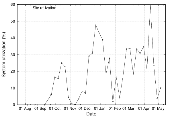

Workload is from August 1st 2004 to May 15th 2005. We have a cluster containing 140 CPUs since September 15th. This can be visible in the figure 2, 3(a) and 3(b), where we notice that the number of jobs sent increases. Statistics are obtained from the PBS log files. PBS log files are well structured for data analysis. An AWK script is used to extract information from PBS log files. AWK acts on lines matched by regular expressions. We do not have information about users Login time because users send jobs to our cluster from an User Interface (UI) of the EGEE Grid and not directly.
4.1 Running time


| Group | Mean | Standard | Number |
|---|---|---|---|
| Deviation | of jobs | ||
| Biomed | 5417 | 22942.2 | 108197 |
| Dteam | 222 | 3673.6 | 94474 |
| LHCb | 2072 | 7783.4 | 9709 |
| Atlas | 13071 | 28788.8 | 7979 |
| Dzero | 213 | 393.9 | 1332 |
During 280 days, our site received 230474 jobs from which 94474 Dteam jobs and 108197 Biomed jobs (table 2). For all these jobs there are 23208 jobs that failed and were dequeued. It appears that jobs are submitted irregularly and by bursts, that is lot of jobs submitted in a short period of time followed by a period of relative inactivity. From the logs, there are not much differences between CPU time and total time, so it means that jobs sent to our cluster are really CPU intensive jobs and not I/O intensive. Dteam jobs are mainly short monitoring jobs but all Dteam jobs are not regularly sent jobs. We have 6784.6 days CPU time consumed by Biomed for 108197 jobs (Mean of one hour and half per jobs, table 2). Repartition of cumulative job duration distributions for Biomed VO is shown on figure 4. The duration of about 70% of Biomed jobs are less than 15 minutes and 50% under 10 seconds, there are a dominant number of small running jobs but the distribution is very wide as shown by the high standard deviation compared to the mean in table 2.
| Queue | Mean | Standard | CV |
|---|---|---|---|
| Deviation | |||
| Test | 31.0 | 373.6 | 12.0 |
| Short | 149.5 | 1230.5 | 8.2 |
| Long | 2943.2 | 11881.2 | 4.0 |
| Day | 6634.8 | 25489.2 | 3.8 |
| Infinite | 10062.2 | 30824.5 | 3.0 |
Users submit their jobs with an estimated run length. For relationships between execution time and requested job duration and its accuracy see [19]. To sum up estimated jobs duration are essentially inaccurate. It is in fact an upper bound for job duration which could in reality take any value below it. Table 3 shows for each queue the mean running time, its standard deviation and coefficient of variation (CV) which is the ratio between standard deviation and the mean. CV decreases as the queue maximum runtime increase. This means that jobs in shorter queues vary a lot in their duration compared to longer jobs and we can expect that more the upper bound given is high the more confidence in using the queue mean runtime as a an estimation we could have.
A commonly used method for modelling duration distribution is to use log-uniform distribution. Figures 4(a) and 4(b) show the fraction of Dteam and Biomed jobs with duration less than some value. Job duration has been modelled with a multi-stage log-uniform model in [20] which is piecewise linear in log space. In this case Dteam and Biomed job duration could be approximated respectively with a 3 and a 6 stages log-uniform distribution.
4.2 Waiting time
| Group | Mean | Stretch | Standard | CV |
|---|---|---|---|---|
| Deviation | ||||
| Biomed | 781.5 | 0.874 | 16398.8 | 20.9 |
| Dteam | 1424.1 | 0.135 | 26104.5 | 18.3 |
| LHCb | 217.7 | 0.905 | 2000.7 | 9.1 |
| Atlas | 2332.8 | 0.848 | 13052.1 | 5.5 |
| Dzero | 90.7 | 0.701 | 546.3 | 6.0 |
| Queue | Mean | Standard | CV | Number |
|---|---|---|---|---|
| Deviation | of jobs | |||
| Test | 33335.9 | 148326.4 | 4.4 | 45760 |
| Short | 1249.7 | 27621.8 | 22.1 | 81963 |
| Long | 535.1 | 5338.8 | 9.9 | 32879 |
| Day | 466.8 | 8170.7 | 17.5 | 19275 |
| Infinite | 1753.9 | 24439.8 | 13.9 | 49060 |
Table 4 shows that jobs coming from the Dteam group are the more unfairly treaten. Dteam group sends short jobs very often, Dteam jobs are then all placed in queue waiting that long jobs from other groups finished. Dzero group sends short jobs more rarely and is also less penalized than Dteam because there are less Dzero jobs that are waiting together in queue before being treated. The best treated group is LHCb with not very long running jobs (average of about 34 minutes) and one job about every 41 minutes. The best behavior to reduce waiting time per jobs seems to send jobs that are not too short compared to the waiting factor, and send not too very often in order to avoid that they all wait together inside a queue. Very long jobs is not a good behavior too as the scheduler delay them to run shorter one if possible.
Table 5 shows the mean waiting time per jobs on a given queue. There is a problem with such a metric, for example: Consider one job arriving on a cluster with only one free CPU, it will run on it during a time with no waiting time. Consider now that this job is splitted in shorter jobs (numbered ) with equal total duration . Then the waiting time for the job number will be , and the total waiting time . So the more a job is splitted the more it will wait in total. Another metric that does not depend on the number of jobs is the total waiting time divided by the number of jobs and by the total job duration. Let note this normalized waiting time, We obtain:
| (4.1) |
| Queue | Group | ||
|---|---|---|---|
| Test | 2.35e-2 | Biomed | 1.58e-5 |
| Short | 1.02e-4 | Dteam | 6.79e-5 |
| Long | 5.53e-6 | LHCb | 1.08e-5 |
| Day | 3.65e-6 | Atlas | 2.23e-5 |
| Infinite | 3.55e-6 | Dzero | 31.9e-5 |
With this metric, the Test queue is still the most unfairly treated and the Infinite queue has the more benefits compared to the other queues. Dteam group is again bad treated because their jobs are mainly sent to the Test queue. The more unfairly treated group is Dzero.
4.3 Arrival time

| Group | Mean | Standard | CV |
|---|---|---|---|
| (seconds) | Deviation | ||
| Biomed | 223.6 | 5194.5 | 23.22 |
| Dteam | 256.2 | 2385.4 | 9.31 |
| LHCb | 2474.6 | 39460.5 | 15.94 |
| Atlas | 2824.1 | 60789.4 | 21.52 |
| Dzero | 5018.7 | 50996.6 | 10.16 |
Job arrival daily cycle is presented in figure 5. This figure shows the number of arrival depending on job arrival hours, with a 10 minutes sampling. Clearly users prefer to send their jobs at o’clock. In fact we receive regular monitoring jobs from the VO Dteam. The monitoring jobs are submitted every hour from goc.grid-support.ac.uk. Users are located in all Europe, so the effect of sending at working hours is summed over all users timezones. However the shape is similar compared to other daily cycle, during night (before 8am) less jobs are submitted and there is an activity peak around midday, 2pm and 4pm.
Table 7 shows the moments of interarrival time for each group. CV is much higher than , this means that arrivals are not Poisson processes and are very irregularly distributed. For instance we could receive jobs in minutes followed by nothing during the next minutes. In this case we have a mean interarrival time of minutes but in fact when jobs arrived they arrived every minutes.
Figure 3(a) shows the system utilization of our cluster during each week. There are a maximum of 980 CPU days consumed each week for 140 CPUs. We have a highly varying cluster activity.
4.4 Frequency analysis


Job arrival rate is a common measurement for a site usage in queuing theory. Figures 6(a) and 6(b) present the job arrival rate distribution. It is the number of time jobs are submitted during interval length of 5 minutes. They show that most of the time the cluster does not receive jobs but jobs arrived grouped. Users actually submit groups of jobs and not stand-alone jobs. It explains the shape of the arrival rate: it fastly decreases but too slowly compared to a Poisson distribution. Poisson distribution is usually used for modelling the arrival process but evidences are against that fact [21].
Dteam monitoring jobs are short and regular jobs, there is no need of a special arrival model for such jobs. What we observe for other kind of jobs is that the job arrival law is not a Poisson Law (see table 7 where ) as for instance a web site traffic [22]. What really happens is that users come using the cluster from an User Interface during some time interval. During this time they send jobs to the cluster. Users log to an User Interface machine in order to send their jobs to a RB that dispatch them to some CEs. Note that one can send jobs to our cluster only from an User Interface, it means for instance that jobs running on a cluster cannot send secondary jobs. On a computing site we do not have this user login information, but only job arrival.
First we look at modelling user arrival and submission behavior. Secondly we show that the model proposed shows good results for a group behavior.
5 Model
5.1 Login model
In this section we begin to model user Login/Logout behavior from the Grid job flow (figure 1). We neglect the case where an user has multiple login on different UI at the same time. We mean that a user is in the state Login if he is in the state of sending jobs from an UI to our cluster, else he is in the state Logout.

Markov chains are like automatons with for each state a probability of transition. One property of Markov chains is that future states depend only on the current state and not on the past history. So a Markov state must contains all the information needed for future states. We decided to model the Login/Logout behavior as a continuous Markov chain. During each , a Logout user has a probability during of to login and a Login user has a probability during of to logout (see figure 7). is called the Login rate and is called the Logout rate.
All these parameters could vary over time as we see with the variation of the week job arrival (figure 3(a)) or during day time (figure 5) The model proposed could be used more accurately with non-constant parameters at the expense of more calculation and more difficult fitting. For example, one could numerically use Fourier series for the Login rate or for the submittal rate to model this daily cycle. We use now constant parameters for calculation, looking for general properties.
We would like to have the probabilities during time that the user is logged or not logged. Let and be respectively probability that the user is logged or not logged at time t. We have from the modelling:
| (5.1) | |||||
| (5.2) | |||||
At equilibrium we have no variation so
| (5.3) | |||
| (5.4) |
We obtain:
| (5.5) | ||||
| (5.6) |
5.2 Job submittal model
During period when users are logged they could submit jobs. We model the job submittal rate for one user as follows: During when the user is logged he has a probability of to submit a job. With we have a delayed Poisson process, with no jobs are submitted. The full model is shown at figure 8, it shows all the possible outcomes with corresponding probabilities from one of the possible state to the next after a small period . Numbers inside circles are the number of jobs submitted from the start. Login states are below and Logout states are at the top. We have:

- •
is the probability to be in the state “User is not logged at time t and n jobs have been submitted between time 0 and t.”
- •
is the probability to be in the state “User is logged at time t and n jobs have been submitted between time 0 and t.”
- •
is the probability to be in the state “n jobs have been submitted between time 0 and t.” We have .
From the model, we obtain with the same method as before this recursive differential equation:
| (5.7) | |||||
| (5.8) | |||||
| (5.9) |
This results to the following recursive equation (in case the parameters are constants, is a constant)
| (5.10) |
We take a look at the probability of having no job arrival during an interval of time which is and . is the the probability that no jobs have been submitted between arbitrary time 0 and t. So from the above model, we have:
| (5.11) |
At arbitrary time we could be in the state Login with probability and in the state Logout with the probability . We have from the results above:
| (5.12) | ||||
| (5.13) |
Finally we obtain the result.
| (5.14) |
Where
| (5.15) | ||||
| (5.16) | ||||
| (5.17) |
With or , we obtain that no jobs are submitted . With , this is a Poisson process and . Note that during a period of there are in average jobs submitted, we have also for small period ,
| (5.19) |
We have also
| (5.20) | ||||
| (5.21) |
could be estimated by splitting the arrival processes in intervals of duration and estimating the ratio of intervals with no arrival. The error of this estimation is linear with . Another issue is that the logs precision is not below one second.
5.3 Model characteristics
We have also these interesting properties:
| (5.22) | |||||
| (5.23) | |||||
| (5.24) | |||||
| (5.25) |
Probability distribution of the duration between two jobs arrival is called an interarrival process. Interarrival process is a common metric in queuing theory. We have with the initial condition that user just submits a job. This implies that user is logged.
| (5.26) |
| (5.27) |
| (5.28) |
We have because
| (5.29) |
So , and we have an hyper-exponential interarrival law of order 2 with parameters . This result is coherent with other experimental fitting results [23] Moreover any hyper-exponential law of order 2 may be modelled with the Markov chain described in figure 8 with parameters
Let calculate the mean interarrival time. Probability to have an interarrival time between and is . The mean is
| (5.30) | |||||
| (5.31) |
Let compute the variance of interarrival distribution.
| (5.32) | |||||
| (5.33) | |||||
| (5.34) | |||||
| (5.35) |
Another interesting property is the number of jobs submitted by this model during a Login period. Let be the probability to receive jobs during a Login period. We have:
| (5.36) | |||||
| (5.37) |
This is a geometric law. The mean number of jobs submitted by Login period is .
5.4 Group model
Groups are composed of users, either regular users sending jobs at regular time or users with a Login/Logout like behavior. Metrics defined below as the mean number of jobs sent by Login state, the mean submittal rate and probability of Login could represent an user behavior.

Figure 9 shows the sorted distribution of users submittal rate (). Except for the highest values it is quite a straight line in logspace. This observation could be included in a group model.
6 Simulation and validation


| Name | Error | |||
|---|---|---|---|---|
| Biomed user 1 | 0.0837 | 0.02079 | 2.1e-4 | 4.929e-3 |
| Biomed user 2 | 0.0620 | 0.01188 | 1.2e-4 | 3.534e-3 |
| Biomed user 3 | 0.0832 | 0.02475 | 2.5e-4 | 1.1078e-2 |
| Biomed user 4 | 0.0365 | 1.4285e-3 | 1.075e-4 | 8.78e-2 |


We have done a simulation in Scheme [24] directly using the Markov model. We began by fitting users behavior from the logs with our model. Like the frequency obtained from the logs, the model shows a majority of intervals with no job arrival, possibly followed by a relatively flat area and a fast decreases. Some fitting results are presented in figures 10. Norm used to fit real data is the maximum difference between the two cumulative distributions. We fitted the frequency data for each user.
During a period of there are in average jobs submitted. We evaluate the value of which is the average number of jobs submitted by seconds. We use that value when doing a set of simulation in order to fit a known real user probability distribution. We have two free parameters, so we vary between 0.0 and 1.0 and which the inverse is the average time an user is Logout. Some results obtained are shown in figures 10.
parameter decides of the frequency length of the curve. Without the Login behavior we would have obtained a classic Poisson curve of parameter. is the mean interarrival time during Login period. An idea to evaluate would be to evaluate the job arrival rate during Login periods, but we lack that Login information.
and are the Logout and Login parameters. What is really important is the ratio which is . This is the ratio between time user is active on the cluster and total time. and are measures of the deviation from a classic Poisson law. For instance, the mean number of jobs submitted by Login period is and the mean job submittal rate is . For a same we could have very different scenarios. A user could be active for long time but rarely logged and another user could be active for short period with frequent login. is the mean Login time, is the mean Logout time.
The probability is essential for studying job arrival time. is the probability that between time and we have received at least one job. It is easier to fit the distribution for an user than the interarrival distribution because we have more points. Figure 11(a) shows a typical graph of for a Biomed user. It shows for instance that for intervals of 10000 seconds, this Biomed user has a probability of about 0.2 to submits one or more jobs. We have fitted this probability with hyper-exponential curve, that is a summation of exponential curves. There was too much noises for high interval time to fit that curve. In fact errors on are linear with . So we have smoothed the curve before fitting by averaging near points. for this user was fitted with a sum of two exponentials.
It seems that more than the Login/Logout behavior there is also a notion of user activity. For example during the preparation of jobs or analysis phase of the results an user does not use the Grid and consequently the cluster at all. More than the Login and Logout state an Inactive state could be added to the model if needed.
6.1 Other workloads comparison
User number 3 is the most active user from the NASA Ames iPSC/860 workload †† † The workload log from the NASA Ames iPSC/860 was graciously provided by Bill Nitzberg. The workload logs from DAS2 were graciously provided by Hui Li, David Groep and Lex Wolters. The workload log from the SDSC Blue Horizon was graciously provided by Travis Earheart and Nancy Wilkins-Diehr. All are available at the Parallel Workload Archives http://www.cs.huji.ac.il/labs/parallel/workload/. Figure 11(b) shows its probability, it is clearly hyper-exponential of order 2, as other users like number 22 and 23. Other users like number 12 and 15 are more classical Poissonian users.
DAS2 Clusters (see note † ‣ 6.1) used also PBS and MAUI as their batch system and scheduler. The main difference we have with them is that they use Globus to co-allocate nodes on different clusters. We only have bag of tasks applications which interacts together in a pipeline way by files stored on SEs. Their fs0 144 CPUs cluster is quite similar with ours. Figure 11(c) shows the probability for their most active user and corresponding hyper-exponential fitting or order 2.
7 Related works
Our Grid environment is very particular and different from common cluster environment as parallelism involved requires no interaction between processes and degree of parallelism is one for all jobs.
To be able to completely simulate the node usage we need not only the jobs submittal process but also the job duration process. Our runtime model is similar with the Downey model [20] for runtime which is composed of linear pieces in logspace. There is a strong correlation between successive jobs running time but it seems unlikely that a general model for duration may be made because it depends highly on algorithms and data used by users.
Most other models use Poisson distribution for interarrival distribution. But evidences, like CV be much higher than one, demonstrate that exponential distributions does not fit well the real data [25, 26]. The need of a detailed model was expressed in [27]. With constant parameters our model exhibits a hyper-exponential distribution for interarrival rate and justify such a distribution choice. One strong benefit of our model is that it is general and could be used numerically with non-constant parameters at the expense of difficult fitting.
8 Discussion
What could be stated is that job maximum run times provided by users are essentially inaccurate, some authors are even not using this information for scheduling [2]. Maybe a better concept is the relative urgency of a job. For example on a grid software managers are people responsible for installing software on cluster nodes by sending installation jobs. Software manager jobs may be regarded as more urgent than other jobs type. So sending jobs with an estimated runtime could be replaced by sending jobs with an urgency parameter. That urgency could be established in part as a site policy. Each site administrator could define some users classes for different kind of jobs and software used with different jobs priorities. For instance a site hosted in some laboratory might wish to promote its scientific domain more than other domain, or some specific applications might need quality of services like real time interaction.
Another idea for scheduling is to have some sort of risk assessment measured during the scheduler decision. This risk assessment may be based on blocking probabilities obtained either from the logs or from some user behavior models. For example, it could be wise to forbid that a group or an user takes all the cluster at a given time but instead to let some few percents of it open for short jobs or low CPU consuming jobs like monitoring.
Information System shows for a site the number of job currently running and waiting. But it is not really the relevant metric in an on-line environment. A better metric for a cluster is the computing flow rate input and the computing flow rate capacity. A cluster is able to treat some amount of computation per unit of time. So a cluster is contributing to the Grid with some computation flow rate (in GigaFLOPS or TeraFLOPS). As with classical queuing theory if the input rate is higher than the capacity, the site is overloaded and the global performances are low due to jobs waiting to be processed. What happens is that the site receive more jobs that is is able to treat in a given time. So the queues begin to grow and jobs have to wait more and more before being started, resulting in performance decay. Similarly when the computation submitted rate is lower than the site capacity the site is under-used. Job submittal have also to be fairly distributed according to the site capacity. For example, a site that is twice bigger than another site have to receive twice more computing request than the other site. But there is a problem to globally enforce this submittal scheme on all the Grid. This is why a local site migration policy may be better than a central migration policy done with the RB.
To be more precise there are two different kinds of cluster flow rate metrics, one is the local flow rate and the other one is the global flow rate. The local computing flow rate is the flow rate that one job sees when reaching the site. The global flow rate is the computing flow rate a group of jobs see when reaching the site. That global flow rate is also the main measurement for meta-scheduling between sites. These two metrics are different, for instance we could have a site with a lot of slow machines (low local flow rate and big global flow rate) and another site with only few supercomputers (big local flow rate and low global flow rate). But the most interesting metric for one job is the local flow rate. This means that if each job wants individually to be processed at the best local flow rate site, this site will saturate and be globally slow.
As far as all users and groups computation total flow rate is less than the site global flow rate or site capacity, there is no real fairness issue because there is no strife to access the site resources, there is enough for all. The problem comes when the sum of all computation flow rate is greater than the site capacity, firstly this globally reduces the site performance, secondly the scheduler must take decision to share fairly these resources. The Grid is an ideal tool that would allow to balance the load between sites by migrating jobs [2]. A site that share their resources and is not saturated could discharge another heavily loaded site. Some kind of local site flow control could maintain a bounded input rate even with fluctuating jobs submittal. For instance fairness between groups and users could be maintained by decreasing the most demanding input rate and distributing it to other less saturated sites.
Another benefits is that applications computing flow rates may be partly expressed by users in their job requirements. Computing flow rate takes into account both the jobs sizes and their time limits. Fairness between users is then ensured if whatever may be flow values asked by each user, part granted to each penalizes no other one. Computing flow rate granted by a site to an application may depend on the applications degree of parallelism, that is for the moment the number of jobs. For instance it may be more difficult to serve an application composed of only one job asking for a lot of computing flow rate than to serve an application asking the same computing flow rate but composed of many jobs. Urgency is not totally measured by a computing flow rate. For example a critical medical application which is a matter of life or death arriving on a full site has to be treated in priority. Allocating flow rates between users and groups has to be right and to take under account priority or urgency issues.
To use a site wisely users have to bound their computational flow rate and to negotiate it with site managers. A computing model has to be defined and published. These remarks are important in the case of on-line computing like Grids where meta-scheduling strategy have to take a lot of parameters into account. General on-line load balancing and scheduling algorithms [28, 29, 30, 31] may be applied. The problem of finding the best suited scheduling policy is still an open problem. A better understanding of job running time is necessary to have a full model.
The LCG middleware allows users to send their jobs to different nodes. This is done by the way of a central element called a Resource Broker, that collects user’s requests and distributes them to computing sites. The main purpose is to match the available resources and balance the load of job submittal requests. Jobs are better localized near the data they need to use.
We would like to advise instead a peer to peer [32] view of the Grid over a centralized one. In this view computing sites themselves work together with other computing sites to balance the average workload. Not relying on dependent services greatly improves the reliability and adaptability of the whole systems. That kind of meta-scheduling have to be globally distributed as stated by Dmitry Zotkin and Peter J. Keleher [12]:
In a distributed system like Grid, the use of a central Grid scheduler‡‡ ‡ like the Resource Broker used in LCG middleware may result in a performance bottleneck and lead to a failure of the whole system. It is therefore appropriate to use a decentralized scheduler architecture and distributed algorithm.
gLite [33] is the next generation middleware for Grid computing. gLite will provide lightweight middleware for Grid computing. The gLite Grid services follow a Service Oriented Architecture which will facilitate interoperability among Grid services. Architecture details of gLite could be viewed in [11]. The architecture constituted by this set of services is not bound to specific implementations of the services and although the services are expected to work together in a concerted way in order to achieve the goals of the end-user they can be deployed and used independently, allowing their exploitation in different contexts. The gLite service decomposition has been largely influenced by the work performed in the LCG project. Service implementations need to be inter-operable in such a way that a client may talk to different independent implementations of the same service. This can be achieved in developing lightweight services that only require minimal support from their deployment environment and defining standard and extensible communication protocols between Grid services.
9 Conclusion
So far we have analyzed the workload of a Grid enabled cluster and proposed an infinite Markov-based model that describes the process of jobs arrival. Then a numerical fitting has been done between the logs and the model. We find a very similar behavior compared to the logs, even bursts were observed during the simulation.
Acknowledgments
The cluster at LPC Clermont-Ferrand was funded by Conseil Régional d’Auvergne within the framework of the INSTRUIRE project (http://www.instruire.org)
References
- [1] Dror G. Feitelson. Workload modeling for performance evaluation. In Maria Carla Calzarossa and Salvatore Tucci, editors, Performance Evaluation of Complex Systems: Techniques and Tools, pages 114–141. Springer-Verlag, Sep 2002. Lect. Notes Comput. Sci. vol. 2459.
- [2] Darin England and Jon B. Weissman. Costs and benefits of load sharing in the computational grid. In Dror G. Feitelson and Larry Rudolph, editors, Job Scheduling Strategies for Parallel Processing. Springer-Verlag, 2004.
- [3] M. Garey and D.S. Johnson. Computers and Intractability: A Guide to the Theory of NP-Completeness. Freeman, San Francisco, CA., 1979.
- [4] Stephan Mertens. The easiest hard problem: Number partitioning. In A.G. Percus, G. Istrate, and C. Moore, editors, Computational Complexity and Statistical Physics, New York, 2004. Oxford University Press.
- [5] Dror Feitelson School. Parallel job scheduling — a status report. In Dror G. Feitelson, Larry Rudolph, and Uwe Schwiegelshohn, editors, Job Scheduling Strategies for Parallel Processing, pages 1–16. Springer Verlag, 2004.
- [6] Dror G. Feitelson and Larry Rudolph. Parallel job scheduling: Issues and approaches. In Dror G. Feitelson and Larry Rudolph, editors, Job Scheduling Strategies for Parallel Processing, pages 1–18. Springer-Verlag, 1995. Lect. Notes Comput. Sci. vol. 949.
- [7] David Jackson, Quinn Snell, and Mark Clement. Core algorithms of the Maui scheduler. In Dror G. Feitelson and Larry Rudolph, editors, Job Scheduling Strategies for Parallel Processing, pages 87–102. Springer Verlag, 2001. Lect. Notes Comput. Sci. vol. 2221.
- [8] Brett Bode, David M. Halstead, Ricky Kendall, and Zhou Lei. The Portable Batch Scheduler and the Maui Scheduler on Linux Clusters, USENIX Association. 4th Annual Linux Showcase Conference, 2000.
- [9] S. Agostinelli et al. Geant 4 (GEometry ANd Tracking): a Simulation toolkit. Nuclear Instruments and Methods in Physics Research, pages 250–303, 2003.
- [10] Ian Foster and Carl Kesselman. Globus: A metacomputing infrastructure toolkit. The International Journal of Supercomputer Applications and High Performance Computing, 11(2):115–128, Summer 1997.
- [11] EGEE Design Team. EGEE middleware architecture, EGEE-DJRA1.1-476451-v1.0, August 2004. Also available as https://edms.cern.ch/document/476451/1.0.
- [12] Dmitry Zotkin and Peter J. Keleher. Job-length estimation and performance in backfilling schedulers. In HPDC, 1999.
- [13] Antonio Delgado Peris, Patricia Méndez Lorenzo, Flavia Donno, Andrea Sciabà, Simone Campana, and Roberto Santinelli. LCG User guide, 2004.
- [14] G. Avellino, S. Beco, B. Cantalupo, A. Maraschini, F. Pacini, M. Sottilaro, A. Terracina, D. Colling, F. Giacomini, E. Ronchieri, A. Gianelle, R. Peluso, M. Sgaravatto, A. Guarise, R. Piro, A. Werbrouck, D. Kouřil, A. Křenek, L. Matyska, M. Mulač, J. Pospíšil, M. Ruda, Z. Salvet, J. Sitera, J. Škrabal, M. Vocu̇, M. Mezzadri, F. Prelz, S. Monforte, and M. Pappalardo. The datagrid workload management system: Challenges and results. Kluwer Academic Publishers, 2004.
- [15] Dror G. Feitelson and Larry Rudolph. Toward convergence in job schedulers for parallel supercomputers. In Dror G. Feitelson and Larry Rudolph, editors, Job Scheduling Strategies for Parallel Processing, pages 1–26. Springer-Verlag, 1996. Lect. Notes Comput. Sci. vol. 1162.
- [16] Su-Hui Chiang, Andrea Arpaci-Dusseau, and Mary K. Vernon. The impact of more accurate requested runtimes on production job scheduling performance. In Dror G. Feitelson, Larry Rudolph, and Uwe Schwiegelshohn, editors, Job Scheduling Strategies for Parallel Processing, pages 103–127. Springer Verlag, 2002. Lect. Notes Comput. Sci. vol. 2537.
- [17] Maria Calzarossa and Giuseppe Serazzi. Workload characterization: A survey. Proc. IEEE, 81(8):1136–1150, 1993.
- [18] Steve J. Chapin, Walfredo Cirne, Dror G. Feitelson, James Patton Jones, Scott T. Leutenegger, Uwe Schwiegelshohn, Warren Smith, and David Talby. Benchmarks and standards for the evaluation of parallel job schedulers. In Dror G. Feitelson and Larry Rudolph, editors, Job Scheduling Strategies for Parallel Processing, pages 67–90. Springer-Verlag, 1999. Lect. Notes Comput. Sci. vol. 1659.
- [19] Walfredo Cirne and Francine Berman. A comprehensive model of the supercomputer workload, 2001.
- [20] Allen B. Downey and Dror G. Feitelson. The elusive goal of workload characterization. Perf. Eval. Rev., 26(4):14–29, 1999.
- [21] Dror G. Feitelson and Bill Nitzberg. Job characteristics of a production parallel scientific workload on the NASA Ames iPSC/860. In Dror G. Feitelson and Larry Rudolph, editors, Job Scheduling Strategies for Parallel Processing, pages 337–360. Springer-Verlag, 1995. Lect. Notes Comput. Sci. vol. 949.
- [22] Vern Paxson and Sally Floyd. Wide area traffic: the failure of Poisson modeling. IEEE/ACM Transactions on Networking, 3(3):226–244, 1995.
- [23] Hui Li, David Groep, and Lex Wolters. Workload characteristics of a multi-cluster supercomputer. In Dror G. Feitelson, Larry Rudolph, and Uwe Schwiegelshohn, editors, Job Scheduling Strategies for Parallel Processing. Springer Verlag, 2004.
- [24] Richard Kelsey, William Clinger, and Jonathan Rees (Editors). Revised5 report on the algorithmic language Scheme. ACM SIGPLAN Notices, 33(9):26–76, 1998.
- [25] Dror G. Feitelson. Metrics for parallel job scheduling and their convergence. In Dror G. Feitelson and Larry Rudolph, editors, Job Scheduling Strategies for Parallel Processing, pages 188–205. Springer Verlag, 2001. Lect. Notes Comput. Sci. vol. 2221.
- [26] Joefon Jann, Pratap Pattnaik, Hubertus Franke, Fang Wang, Joseph Skovira, and Joseph Riodan. Modeling of workload in MPPs. In Dror G. Feitelson and Larry Rudolph, editors, Job Scheduling Strategies for Parallel Processing, pages 95–116. Springer Verlag, 1997. Lect. Notes Comput. Sci. vol. 1291.
- [27] David Talby, Dror G. Feitelson, and Adi Raveh. Comparing logs and models of parallel workloads using the co-plot method. In Dror G. Feitelson and Larry Rudolph, editors, Job Scheduling Strategies for Parallel Processing, pages 43–66. Springer Verlag, 1999. Lect. Notes Comput. Sci. vol. 1659.
- [28] Yossi Azar, Bala Kalyansasundaram, Serge A. Plotkin, Kirk Pruhs, and Orli Waarts. On-line load balancing of temporary tasks. J. Algorithms, 22(1):93–110, 1997.
- [29] Yossi Azar, Andrei Z. Broder, and Anna R. Karlin. On-line load balancing. Theoretical Computer Science, 130(1):73–84, 1994.
- [30] A. Bar-Noy, A. Freund, and J. Naor. New algorithms for related machines with temporary jobs. In E.K. Burke, editor, Journal of Scheduling, pages 259–272. Springer-Verlag, 2000.
- [31] Tak-Wah Lam, Hing-Fung Ting, Kar-Keung To, and Wai-Ha Wong. On-line load balancing of temporary tasks revisited. Theoretical Computer Science, 270(1–2):325–340, 2002.
- [32] Nazareno Andrade, Walfredo Cirne, Francisco Brasileiro, and Paulo Roisenberg. OurGrid: An approach to easily assemble grids with equitable resource sharing. In Proceedings of the 9th Workshop on Job Scheduling Strategies for Parallel Processing, June 2003.
- [33] EGEE Design Team. Design of the EGEE middleware grid services. EGEE JRA1, 2004. Also available as https://edms.cern.ch/document/487871/1.0.