Position resolution and particle identification with the ATLAS EM calorimeter
Abstract
In the years between 2000 and 2002 several pre-series and series modules of the ATLAS EM barrel and end-cap calorimeter were exposed to electron, photon and pion beams. The performance of the calorimeter with respect to its finely segmented first sampling has been studied. The polar angle resolution has been found to be in the range . The rejection has been measured to be about 3.5 for 90% photon selection efficiency at GeV/c. e- separation studies have indicated that a pion fake rate of (0.07-0.5)% can be achieved while maintaining 90% electron identification efficiency for energies up to 40 GeV.
Keywords:
Calorimeters , particle physicsPACS
29.40.Vj , 06.30.Bp, , , , , , , , , , , , , , , , , , , , , , , , , , , , , , , , , , , , , , , , , , , , , , , , , , , , , , , , , , , , , , , , , , , , , , , , , , , , , , , , , , , , , , , , , , , , , , , , , , , , , , , , , , ,
1 Introduction
The CERN Large Hadron Collider (LHC) is a proton-proton collider with 14 TeV centre of mass energy and design luminosity of . ATLAS is a LHC experiment designed to maximise the discovery potential for new physics phenomena such as Higgs bosons and supersymmetric particles, while keeping the capability of high-accuracy measurements of known objects such as heavy quarks and gauge bosons.
A very challenging mass region for Higgs discovery at the LHC lies between the limit reached by the LEP2 detectors at 114.4 GeV [1] and GeV. In this region, the decay is one of the most promising discovery channels. Its observation requires an excellent performance of the electromagnetic calorimeter in terms of energy resolution, precision of angular measurement and particle identification capability.
The electromagnetic calorimeter in the ATLAS experiment is a lead-liquid argon sampling calorimeter with accordion shaped absorbers and electrodes. Liquid argon technology has been chosen because of its intrinsic linear behaviour as function of the deposited energy, stability of the response and radiation tolerance.
In the following, the beam direction defines the axis, and the plane is transverse to the beam direction. The azimuthal angle is measured around the beam axis, and the polar angle is the angle from the beam axis; the pseudorapidity is defined as . The calorimeter has a cylindrical symmetry with a longitudinal segmentation along the radius of the cylinder and transverse segmentation along the pseudorapidity . The central part covering is housed in a separate barrel cryostat. The two end-caps cover the region of . The transverse momentum is measured in the plane. The optimisation of the longitudinal and transverse segmentation of the calorimeter involves balancing performance issues such as electron and photon identification, position resolution, and pile-up and electronic noise contributions against cost and technical constraints such as routing of the signals from the calorimeter volume.
The dominant backgrounds for the electrons and photons identification arise from the production of hadronic jets. The segmentations of the calorimeter [2], sketched in Fig. 1, allow a measurement of the shower shape that are an essential tool in background rejection. In addition, the rejection of spatially isolated signals from high- ’s coming from hadronic jet fragmentation is especially important: ATLAS design goal calls for a factor of three rejection of at a single-photon efficiency of 90% .
At the LHC design luminosity, the beam spread in the coordinate is about a few centimetres. The beam spread contributes to the angular resolution of the the invariant mass. In order to minimise its effects, the photon direction has to be measured in , with a resolution of about 50 mrad/. In the direction, the interaction point is known with a precision of a few microns in the plane, and the azimuthal angle measurement is well constrained. All this requires a fine-grained position-sensitive device to perform angular measurements and discriminate against the two merged photons from the decay. This is done by segmenting the first longitudinal sampling of the barrel (front compartment) into narrow cells of size . For the end-cap, the segmentation of the first sampling is . The other two compartments (middle and back) are segmented with towers of size in the second (third) sampling.

In this paper the performances of barrel and end-cap modules, with respect to the segmentation of their first compartment, are presented. The results are based on analyses of test-beam data taken in 2000 with barrel module 0 (for the rejection calculation, section 4) and between 2001 and 2002 with series modules.
2 Experimental setup
A detailed description of barrel and end-cap modules of the ATLAS electromagnetic calorimeter, and of the signal reconstruction techniques can be found in Refs [3, 4]. Two production modules, P13 for the barrel calorimeter and ECC1 for the end-cap were tested in the CERN H6 and H8 beam lines during several months of tests during 2001-2002. The test setup is similar to the one described in Refs [3, 4].
2.1 Electron run setup
The calorimeter performance was tested using secondary or tertiary electron and pion beams, with momenta ranging from 20 to 245 GeV/c for barrel modules and from 20 to 150 GeV/c for end-cap modules. The beam lines (Fig. 3) were equipped with three scintillators (S1 to S3) in front of the calorimeter for triggering purposes. Four multi-wire proportional chambers(BC1 to BC4) allowed to determine the beam impact point at the calorimeter with a resolution of about 250 m in the direction. The size of the last two scintillators, , defined the beam acceptance. Cryostats housing the modules were mounted on remotely controlled rails that allowed movements in and while ensuring incident angles similar to the ones expected in ATLAS for all positions. A 3 lead absorber, a pion counter, a 5 iron absorber and a muon counter were placed downstream of the cryostat. -scans were done at an electron energy of 245 GeV for the barrel and 120 GeV for the end-cap. Energy scans at fixed positions were also carried out.
2.2 Photon run setup
The calorimeter response to the incident photons was measured using the prototype module M0. The beam line arrangement is illustrated in Fig. 2. Electrons, with a momentum of 50 or 180 GeV/c impinged on a lead target and produced bremsstrahlung photons. A 4 magnet, placed downstream of the target swept away the charged tracks from the photon trajectory. The unaffected photon beam was incident on the module at an angle and position corresponding to and rad. A beam chamber, BC1, was placed before the target and two more, BC2-BC3, downstream of the magnet, in order to reject out of time counts. Beam trigger was provided by a coincidence of signal from two scintillator counters S1 and S2. This second counter could be displaced in the transverse direction with respect to the beam line in order to trigger on deflected electrons of different energy. A thick converter, followed by scintillator S3 to detect photon conversions into pairs, was placed in the photon beam to enrich the data sample of events in which no more than one photon was present; its effect is described more in detail in section 4.5. The calorimeter was positioned 25 m downstream of the target.


It was found that about of material was present along the beamline and acted as additional source of photons [5]. In order to estimate the amount of events for which more than one photon was present, a sample of photons produced with the 180 GeV beam was also recorded without the photon converter.
2.3 Pion run setup
Positively charged pion beams of 20 and 40 GeV/c momentum, provided by the CERN H8 beamline, were used. The beam impinged on series barrel module P15 of the calorimeter at fixed incident angle and position corresponding to and rad. In addition to the usual test-beam setup, a Čerenkov counter was placed in the beam line and filled with He gas at the pressure of bar. The momentum threshold for a pion to generate Čerenkov light was 80 GeV/c and the counter provided an efficient discrimination of incident pions and electrons at 20 and 40 GeV/c beam momenta.
3 Position and polar angle resolution
The data were processed using the signal processing and pattern recognition software EMTB [6] to calculate the position and polar angle resolutions. The event energy and position were reconstructed using the optimal filtering technique [7, 8], with a cluster size of cells for the front and cells for the middle layer. Random, muon- and pion-like events were discarded using trigger and scintillator information. To correct for the energy loss upstream of the calorimeter, the energy deposited in the presampler was weighted by a factor when calculating the total energy deposited (). Longitudinal energy leakage induces a deterioration of the energy resolution, therefore a weight was also applied to the energy deposited in the back sampling:
| (1) |
The parameters and were obtained by minimising the energy resolution for every position [9].
3.1 Position resolution in the direction
-scans with cells at rad for the barrel and rad for the end-cap were taken to study the variation of the position resolution in the direction. Cells for which no optimal filtering coefficients were available were excluded from the analysis; the scanned region was therefore reduced to (barrel) and (end-cap). In addition, cells in the barrel at rad, and , where a large number of events was accumulated, were used to evaluate the variation of the position resolution with respect to the impact point in the cell.
Pions in the beam are expected to deposit lower energy in the calorimeter than electrons. In order to improve the pion rejection, it was required that the peak value of the energy distribution fitted (Fig. 4) to a Gaussian shape with peak value and width is in the range . Additional constraints were imposed on the timing signal coming from the four beam chambers to guarantee a good track reconstruction and rejection of accidental background. Finally, the barycenters of the reconstructed showers in and were required to be within the central cell of a 33 cluster in the middle compartment. About 12% of the events for the barrel module and 9% of the events for the end-cap module remained after all these requirements.

The electron impact position of the beam particle on the calorimeter was calculated performing a linear fit through the points identified by the beam chambers in each event. The resolution for each chamber, obtained from the distribution of the residuals, was used to estimate the uncertainty in the track extrapolation to the front face of the calorimeter. Fitted tracks were extrapolated to the shower barycenter in both front and middle compartments. Except in the case where the electron track originated at the virtual ATLAS interaction point, the different depths of the shower barycenters and the electrodes’ geometry resulted in different extrapolated values of in the front and middle compartments. The chambers’ resolution was estimated to be about 250 m (i.e. in units of pseudorapidity) for both beamlines.
Two methods were used to calculate the cluster position in the calorimeter.
In the first method, the position of an electron cluster in the samplings is the energy-weighted average of the positions of the cells included in the cluster. Due to the steeply falling lateral profile of the EM shower, the finite granularity of the calorimeter induces a systematic shift of the measured shower barycenter towards the centre of the cell. This effect is stronger in the direction, while the energy sharing is larger in the direction because of the accordion shape. In test-beam data, the shower barycenter position measured by the calorimeter can be compared to the position measured by the beam chambers. The resulting distortions of the measured positions were fitted and used to correct the barycenter position. The corrections depended on the beam energy and the direction.
The second method took into account the exponential transverse profile of the shower. Here the average of the positions of the cells included in the cluster was calculated by weighting the individual contributions with the logarithm of the cell energy, according to [10]:
| (2) |
where the index runs over cells belonging to a given cluster in a compartment. In this case,
| (3) |
is the total energy deposited in a given compartment, and is a parameter that defines a minimum fraction of the shower energy in the cell and sets the relative importance of the tails of the shower in the weighting procedure. With this reconstruction the position distortion practically disappears and can be directly compared with without further corrections.
A comparison of versus distributions for the cases of standard and logarithmic weighting (LW) is presented in Fig. 5.

Here, the value of was chosen such that it gives a minimum for the position resolution. For the barrel module, the best value was found to be 2.0 for the front and 4.4 for the middle compartment at rad. For the end-cap module, at rad in the front compartment, the value of was 2.2. A plot showing the variation of the resolution for the front and middle compartments as a function of at rad is presented in Fig. 6.

In the middle compartment the accumulated statistics per cell was sufficient to perform a good fit of the position distortion. It was found that the position correction done using LW for the middle compartment gave results worse by 20 to 60% [11] at 245 GeV.
The case is different for the front compartment; its finer segmentation with respect to the middle compartment implied a much smaller number of events populating a given strip. The fits were therefore more difficult to perform and only possible for the two strips nearest to the impact point of the electron. For these strips it was found that the two weighting methods gave comparable results. In order to analyse the highest possible number of strips, it was decided to use the LW method to correct the reconstruction bias in the front compartment.
3.1.1 Monte Carlo samples
GEANT3 simulation [12], adapted to reproduce ATLAS test-beam events, was used to generate Monte Carlo samples for the barrel module. For each cell rad, about 3000 events were generated. Three samples at rad containing about 10000 events were also used to study cells for which a large number of events was available at and . The Monte Carlo samples were analysed with the EMTB package in which the clustering routine was modified to take into account electronic noise and cross-talk. The cell noise level for presampler, front, middle and back compartments was set to 45, 15, 30 and 25 MeV respectively. The cross-talk was set to 4.1% (1%) between neighbouring front (middle) compartment cells. The comparison of the data and Monte Carlo is illustrated in Fig. 7 and shows a good agreement.


3.1.2 Resolution calculation
For the middle compartment, the correction’s shape was fitted to the function:
| (4) |
where is normalised to the cell width, as illustrated in Fig. 7. For the barrel, the fit was performed to the Monte Carlo samples and the resulting correction applied directly to the data. For the end-cap, the fit was performed directly to the data. The corrected value for the barycenter was then compared with the one obtained by track extrapolation. The resulting distribution was fitted with a sum of two Gaussians, in order to take into account the non-Gaussian tails due to residual accidental hits in the beam chambers, as shown in Fig. 8. The parameters of the two Gaussians were defined by
| (5) |

The resolution of the beam chambers was subtracted in quadrature. The results for the middle and front compartments are summarised in Fig. 9 for barrel and end-cap modules. In the barrel, the position resolution for both compartments does not have strong variation with and agrees well with Monte Carlo simulation. The finer granularity of the front compartment results in a better position resolution. Using the value of the resolution at small for the barrel and the appropriate extrapolation distance for the two compartments, it was possible to estimate the resolution as m for the front and m for the middle compartment. In the end-cap, the worsening of the resolution at large is expected and is due purely to geometrical effects.


3.1.3 Resolution variation within a cell
Using the runs for which a large number of events was accumulated, it was possible to check how the resolution varied within a single cell of the middle compartment. After obtaining the correction from a fit to the Monte Carlo sample, the cell was divided into 10 slices in and the correction applied. Again, the distribution was fitted for each slice to a sum of two Gaussians, and the width of the narrower Gaussian was compared to the prediction of Monte Carlo. The variation of the resolution across a single cell is shown in Fig. 10 for the barrel module at rad. As expected, the resolution is better at the border of the cell because of the better energy sharing among cells in the cluster; the lopsided symmetry is due to the geometric shape of the cell and the variation of the amount of material along .

3.1.4 Resolution energy dependence
For the barrel module, several data samples were studied for a position rad and at several different beam energies in the range of 20 GeV to 245 GeV. The resolution was calculated as described in section 3.1.2, and the resulting variation of the resolution for different beam energy was fitted with a function:
| (6) |
where is the beam energy. The result of the fit is presented in Fig. 11 and Table 1. For the end-cap module, several samples were studied at rad and different energies in the range of 20 GeV to 150 GeV. The results of the fit are shown in Fig. 11 and Table 2.


| (GeV) | |||
|---|---|---|---|
| Strips | |||
| Middle |
| (GeV) | |||
|---|---|---|---|
| Strips | |||
| Middle |
3.2 Polar angle resolution
The knowledge of the shower barycenters in the first two compartments of the calorimeter allowed an extraction of the vertex position and the direction of the incident electron, relying only on calorimeter information. These values can be compared with values measured by the beam chambers (for the data) or generated (for the simulation). The reference frame used in the following is described in Fig. 12.
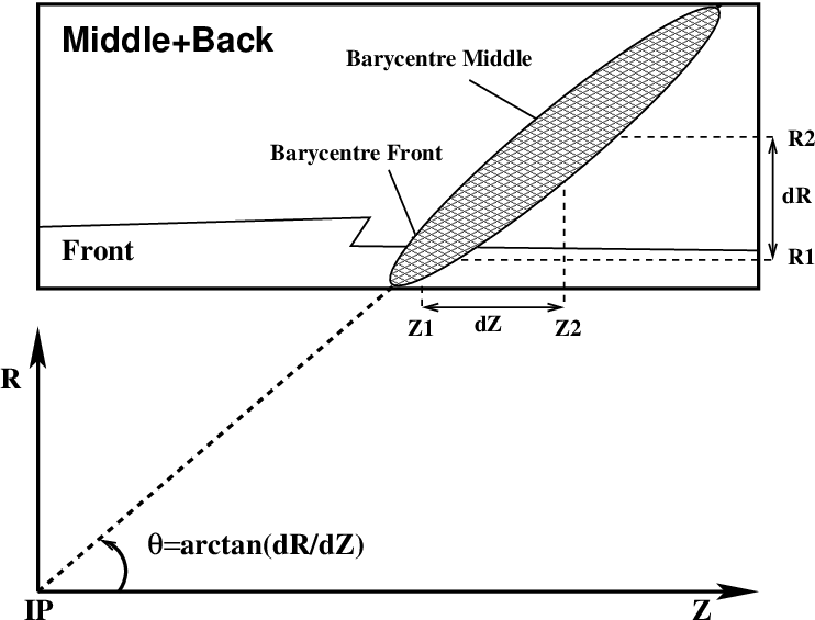
Here, is the coordinate along the ATLAS beam line and is the radial coordinate with respect to the same beam line, found for each cell in using the extrapolation distance to the shower barycenter. The vertex position in is given by:
| (7) |
The direction of the incident electron can be calculated as
| (8) |
where are the angles pointing to the barycenter for the front and middle compartment respectively. The polar angle resolutions were also calculated as function of the beam energy using the energy scan at rad for the barrel and rad for the end-cap. The resulting resolutions are plotted in Figs. 13 and 14.


For both barrel and end-cap, the measured polar angle resolution is in the range 50-60 mrad/, in good agreement with the design expectations.
4 rejection
The rejection is defined as
| (9) |
at fixed photon selection efficiency, where is the pion selection efficiency, and the number of neutral pions before and after the selection requirements. In the present analysis, the requirements were chosen such that the photon selection efficiency on a GeV/c photon sample was 90%. As no beam was available, a -like sample has been produced by superimposing photons according to the kinematics of the decay.
4.1 Event selection
In order to have a sample of photons as clean as possible, only runs taken with the converter placed in the photon beam were used to compute the rejection. To allow tagging, the electron had to hit the sensitive area of the last two beam chambers. The rejection of accidental background and events in which the electron showered before reaching the calorimeter was ensured by the requirement that the signal coming from the beam chambers’ TDCs be consistent with the passage of a single electron. About 30% of the events satisfied all these requirements. To avoid shower overlap, the electron and photon positions had to be separated by more than 3 cells in the middle compartment (i.e. ). The sum of the photon and electron energies had to be consistent with the beam energy, thus allowing the rejection of events in which the photon was lost in the collimator. All these requirements reduced the sample to 5% of its initial size. The rejection of most multi-photon events (i.e. events for which more than one photon was present) was done using as photon veto the scintillator S3 located downstream of the photon converter. In fig. 15 is shown the photon energy as function of the distance between the photon and electron clusters for the two beam energies. Events more than away from the expected distribution were rejected. This last requirement reduced the sample by an additional factor of 3. The energy for each strip was corrected to take into account the 4.1% cross-talk described in section 3.1.1. Finally, further multi-photon event rejection was achieved by requiring the height of the second maximum in the strip energy distribution to be less than 200 MeV, value determined from Monte Carlo simulation (see section 4.3). After all cuts, about 6450 photon events were kept in the sample.

In order to calculate the rejection, pairs of test-beam photons were used to build a decay, modelled according to a simple kinematic simulation at GeV/c and . The simulation provided a set of kinematic configurations, i.e., photon momenta in the laboratory reference frame. The selection was performed in terms of energy and distance between the two photons in the direction. The energies had to match within GeV with the values expected from the kinematic simulation. Their relative distance had to be within 0.03 strip widths in . After this selection, the -like sample was made by superimposing the two photons: their energy deposit was summed strip by strip.
4.2 Monte Carlo samples
GEANT3 simulation [12], adapted to reproduce ATLAS test-beam events, was used to generate a Monte Carlo photon sample, consisting of about 8000 events, at rad, and in the energy range 0-70 GeV. A sample of direct decays was also generated at rad, GeV/c to check the consistency of the method described above.
These Monte Carlo samples were analysed with the EMTB package as described in section 3.1.1. The cross-talk between strips was corrected for in the data, but a consistency check was carried out by introducing cross-talk in the simulated samples instead; the resulting agreement between data and Monte Carlo for the separation was unchanged with respect to the standard analysis.
4.3 rejection calculation
Photons and neutral pions can be separated by analysing the shower shapes in the first sampling of the calorimeter in the region around the shower direction defined by a cluster. A shower generated by a is expected to be wider than a shower generated by a single photon, and may have a second peak in its energy spatial distribution. Several discriminating variables were defined [2, 13]:
- •
shower width on strips in strip units:
where is an index running over the selected number of strips, the strip corresponding to the maximum energy deposit (in the present analysis, shower widths over 3 and 21 strips were considered, called and respectively) ;
- •
energy of the second maximum in the cluster, e2max;
- •
difference of the energy in the strip with the second maximum and the energy deposit in the strip with the minimal value between the first and second maximum, edmax;
- •
energy deposited outside of the shower core,
where is the energy deposit in strips around (and including) the strip with maximum energy deposit.
The distributions of the discriminating variables, for samples of real and simulated photons, are shown in Fig. 16. The choice of a cut at 200 MeV for e2max, to reject multi-photon events, was justified by the data/simulation discrepancy in the tails of both the e2max and edmax distributions; the rejection on the simulated sample was not affected by this requirement.


As can be seen in Fig. 16-e, due to the finite granularity of the detector, the width calculated on 3 strips depends on the impact position of the photon within the strip. This effect was corrected by fitting the distribution of w3st versus the impact position of the photon within the strip, with a polynomial of degree 6; the resulting w3st distribution is presented in Fig. 16-f.
The same variables were calculated for the -like energy distributions, and are presented in Fig. 17. In the case of direct simulation (whose distributions in Fig. 17 are labelled as ‘ MC’), the noise contribution was multiplied by . It can be seen that, due to the separation between the two photons, the average values for the distributions are larger for -like distributions than for photon-like ones. For the present analysis, a candidate was rejected when the values of the discriminating variables were larger than the limits defined by the vertical lines in Fig. 17. Sets of cuts were determined by independently varying the limit for each variable, while retaining 90% selection efficiency on the single photon subsample with GeV/c. The set shown in Fig. 17 was the one that yielded the best rejection.


The discrepancy between data and simulation, especially for the variables eocore and w21st, can be explained by looking at the data/simulation comparisons for the lateral shower profile. In Fig. 18 is shown that the agreement is good for the shower core, i.e., the 3 strips around the maximum, but the discrepancy increases with the distance from the maximum. The non-uniform distribution of dead material located in the beam-line and not described in the Monte Carlo might explain this discrepancy.

As only electron beam energy of 50 and 180 GeV were used to produce the photon beam, the resulting photon energy spectrum was not uniform, but showed a lack of photons with energy around 15 GeV, as detailed in Fig. 19. This affected the reconstruction of pions shown in Fig. 20-a, where the variable , describing the energies of the photons coming from the decay, is plotted for data and simulation. The lack of photons in the distribution for data is reflected by a large dip at 0.25: the rejection was therefore calculated in 6 bins of this variable, in the range 0 to 0.5.

4.4 Results
The photon efficiency was calculated for the photon sample at a 50 GeV/c. A bias in the calculation of the rejection was introduced by the different starting points of the photon energy distributions for data and for the Monte Carlo shown in Fig. 19. The number of photons is significant only for energies greater than 1 GeV in data, making it impossible to estimate the rejection for very asymmetric decays, where one photon carries most of the pion energy. Assuming that the simulation correctly reproduces the photon spectrum at low energy, the distribution for data can be extrapolated using the expected MC shape, and the rejection recalculated taking this correction into account. The difference between the rejection calculated in the second half of the first bin of the distribution and the extrapolation to the full bin was -0.15.
The distribution of the binned rejection factor is presented in Fig. 20-b. The average value, obtained with a sample of 2300 reconstructed pions, was:
| (10) |
where is the number of bins and the rejection in each bin. This value agrees with expectations in Ref [2].

The same procedure was applied to simulated photons. They were paired up to reproduce the kinematic simulation, and the requirements were adapted to take into account the differences between real and simulated distributions. In particular, the cuts were varied in such a way that the same fraction of events was kept after each cut in data and simulation, resulting in an overall photon selection efficiency of %. From the sample of 8000 simulated photons, about 3600 events were reconstructed. The rejection factor , calculated using the same binning as for data, was . The good agreement of the calculated values of this rejection factor for the data and Monte Carlo is shown in Fig. 20-b
4.5 Systematic uncertainties
The impact of the cross-talk was studied by removing the 4.1% cross-talk contribution described in section 4.1. The pion rejection degraded to , in good agreement with expectations [14].
The residual contamination of multi-photon events in the data sample could introduce a bias in the determination of the rejection factor. As the amount of matter before the target was not well known, the contamination could be estimated by comparing the standard sample, in which the converter on the photon beam was present, with another sample where the converter was removed. Assuming that the distribution of events with a certain number of photons is Poissonian, and knowing the converter thickness and, therefore, the photon conversion probability, it is possible to estimate the fraction of multi-photon events in both samples by comparing the absolute number of counts. It was found that the sample without converter contained 72% of single photons, 23% of double photons, 5% of triple photons. For the sample with converter, these fractions were 84%, 14% and 2% respectively. In principle, from these figures it should be possible to extrapolate the value of the rejection to the case without multi-photon contamination; in practice, due to the fact that no runs without converter were taken at low energy, only a comparison for sub-samples could be done. In fact, if one restricts the calculation of the rejection to the region , both photons building the come from the sample at high energy, for which the two setup conditions (with or without converter) were present. The linear extrapolation to no background coming from multiphotons induces a variation in the last bin of .
Finally, the pairing of the photons to build a was tested by calculating the difference in rejection between the direct simulation and the Monte Carlo sample obtained with the method described in section 4. To allow a direct comparison between the samples, the noise level for the direct simulation was multiplied by a factor . The difference in the rejections was found to be +0.23.
5 e- separation
Electromagnetic showers initiated by electrons are expected to be fully contained in the electromagnetic calorimeter. The hadronic showers start at a larger depth of the module and there is often a substantial fraction of the total energy shower leaking into the hadronic calorimeter. However, a fraction of hadron-initiated showers may be fully contained creating a potential for particle misidentification. Therefore it is necessary to use the longitudinal and lateral segmentation of the electromagnetic calorimeter to minimise pion misidentification as electrons while maintaining high electron identification efficiency.
5.1 Clustering and shower profiles
Data were analysed using the standard clustering procedure described in section 3. The shape of the longitudinal shower profile was contained in the information of the energy deposited in each layer of the calorimeter. Additional information was contained in the lateral shower profile, characterised by the number of “hit” cells in each layer, NH(), i.e. the number of cells that contain energy above the noise level. For each cell the noise level was obtained using the random trigger. The noise distribution was fitted with a Gaussian function and the noise level was given by the standard deviation of the fit. It was found to correspond to 44, 12, 32, 21 MeV respectively for the four samplings of the calorimeter in this rapidity region. The minimum energy required for a cell to register a hit corresponded to a cut above the noise level.
In this analysis, the number of hit cells in a given layer was calculated only within the selected cluster. The number of hit cells is quite different for electrons and pions, for the 20 and 40 GeV/c beams, as shown in Fig. 21, and may provide additional discrimination power.
Instead of total energy deposits in the calorimeter, ratios of the energy in each individual layer to the total energy deposited in the cluster, , were used. In general, the number of hit cells and the energy fraction in a given layer are correlated. This correlation shown in Fig. 22 is weak. Thus the number of hit cells provides additional information to a longitudinal profile analysis. The additional information allows for significantly better pion rejection.


Another variable used in the analysis is the fraction of energy deposited in the shower core. To obtain it, the central cell of the middle sampling cluster was projected onto the other layers, and the total energy corresponding to such calorimeter tower calculated. The fraction of energy deposited in the shower core was then defined as .

5.2 Sample purity
To select the electron sample, the ADC counts from the Čerenkov counter were required to be greater than 400, above the pedestal, Pion run samples were normalised to the electron run samples with ADC counts less than 400 according to their total area. The tail of the ADC counts distribution of the pion sample above 400 gave the maximum contamination in the electron sample. The purity of the electron sample was defined as the number of electron sample counts with pion contamination subtracted, divided by the number of electron sample counts, and was found to be better than 99.9%.
The pion sample was selected by requiring the Čerenkov ADC counts to be less than 400 for the pion run data, and its purity was calculated to be better than 99% for all momenta.
5.3 Analysis strategy
The variables used in the analysis are the four energy fractions , the fraction of energy deposited in the shower core , and the number of hit cells in each layer NH(). Assuming that the track momentum is known, one may use it as additional variable, and study separation with samples of the same momentum.
Two analysis methods [15] made use of the variables defined so far. The first method was based on simple cuts to separate electrons of pion signals while keeping the electron identification efficiency at about 90%. The second method relied on a Neural Network (NN) approach using the same variables. In particular, a multi-layer perceptron (MLP) with one hidden layer was used to build the NN. Monte Carlo data were divided into three equal subsamples of a specific momentum and particle type, serving as NN training sample, verification sample and a testing sample. The number of neurons varied with the number of input variables, following the rule of thumb that the number of hidden neurons should be about twice the number of input variables. The neural network results were stable when changing the number of hidden neurons. The error of the output of the NN was checked to avoid over-training.
5.4 Results
The results are summarised in Tables 3 and 4 for analyses based on cuts and Neural Network approach, applied to 20 and 40 GeV electron and pion samples. The pion fake rates for fixed electron efficiency of 90 % are compared for the two methods. For the NN method, a single cut applied on the NN output provides the result. For the cut method, the thresholds were varied on all variables in order to minimise the pion fake rates while preserving the electron identification efficiency.
| 20 GeV with 90% electron efficiency | Fake rate (CUT) | Fake rate (NN) |
|---|---|---|
| Energy ratio | % | % |
| Energy ratio + hit cells | % | % |
| Ratio + hit cells + | % | % |
| 40 GeV with 90% electron efficiency | Fake rate (CUT) | Fake rate (NN) |
|---|---|---|
| Energy ratio | % | % |
| Energy ratio + hit cells | % | % |
| Ratio + hit cells + | % | % |
6 Conclusions
Test-beam data collected in the years 2000-2002 with pre-series and series modules of the ATLAS EM barrel and end-cap calorimeter have shown that the design goals in terms of position and polar angle resolution, rejection and separation can be reached. The position resolution along was measured to be about and (in units of pseudorapidity) for front and middle compartment respectively, allowing to achieve a polar angle resolution in the range . The rejection, in test-beam conditions, was calculated to be for 90% photon selection efficiency at GeV/c, with room for improvement when the systematic errors from irreducible multi-photon background () and building strategy (+0.23) are taken into account. Finally, the study of separation performed at 20 and 40 GeV yielded a fake rate of % and % with a simple cuts method, % and % with a Neural Network method, while maintaining in both cases 90% electron identification efficiency. Significant improvement in separation can be achieved by using the lateral shape of the shower described by the number of hit cells.
Acknowledgements
We are indebted to our technicians for their contribution to the construction and running of the barrel and end-cap modules and the electronics. We would like to thank the accelerator division for the good working conditions in the H6 and H8 beamlines. Those of us from non-member states wish to thank CERN for its hospitality.
References
- [1] R. Barate et al., “Search for the Standard Model Higgs Boson at LEP.” Phys. Lett. B565:61-75,2003.
- [2] ATLAS collaboration, ATLAS: Detector and Physics Performance; Technical Design Report, Volume I and II, CERN LHCC-99-014 and LHCC-99-015.
- [3] B. Aubert et al., “Performance of the ATLAS electromagnetic calorimeter end-cap module 0.” Nucl. Instrum. Meth. A500:178-201,2003.
- [4] B. Aubert et al., “Performance of the ATLAS electromagnetic calorimeter barrel module 0.” Nucl. Instrum. Meth. A500:202-231,2003.
- [5] S. Viret, “ATLAS electromagnetic barrel photon testbeam response compared to GEANT4 simulation.” ATL-LARG-2004-011 (2004).
- [6] R. Lafaye et al., “EMTB User Guide Version 1-9.” ATLAS documentation.
- [7] W.E. Cleland and E.G. Stern, “Signal processing considerations for liquid ionization calorimeters in a high rate environment.” Nucl. Instrum. Meth. A338:467-497, 1994.
- [8] L. Neukermans, PhD Thesis, Laboratoire d’Annecy-le-Vieux de Physique des Particules (LAPP), 2002.
- [9] D. Banfi, M. Delmastro, M. Fanti, “Energy resolution optimization through layers measurements weighting: analytical solutions and numerical strategies.” ATL-LARG-2002-002 (2002).
- [10] T.C. Awes et al., “A simple method of shower localization and identification in laterally segmented calorimeters.” Nucl. Instrum. Meth. A311:130-138, 1992 .
- [11] R. Sacco, “Position resolution of an ATLAS electromagnetic calorimeter module.” ATL-LARG-2003-008 (2003).
- [12] “GEANT: Detector Description and Simulation.” CERN Program Library Long Writeup W5013.
- [13] M. Wielers, “Isolation of Photons.” ATL-PHYS-2002-004 (2002).
- [14] ATLAS collaboration, “Detector and Physics Performance Technical Design Report.” CERN/LHCC 99-14 (1999).
- [15] L. Liu, Y. Gao and R. Stroynowski, “ Separation in the Barrel Electromagnetic Calorimeter with 2002 Test Beam Data.” ATL-LARG-2003-013 (2003).