The Rate of Expansion of Spherical Flames

V. Karlin and G. Sivashinsky Thanks: University of Central Lancashire, Preston, UK Thanks: Tel Aviv University, Tel Aviv, Israel

Abstract

In this paper we investigate the acceleration of the expansion of premixed spherical flames and evolution of the cellular patterns on their surfaces. An asymptotic model is used for the simulations and a spectral numerical algorithm is employed to study flames over large time intervals. Numerous numerical experiments indicate that for large enough time intervals the acceleration of two-dimensional expanding flame ceases and the expansion rate stabilizes to a value significantly exceeding the burning rate. The importance of the effect of forcing was also confirmed and the validity of sectorial simulations of closed flames was studied in order to justify prospective use of the Fourier spectral model for the three-dimensional spherical flames.

1 Introduction

In [1] extensive experimental data on premixed expanding spherical flames have been analysed and it was concluded that starting from a certain moment the averaged flame radius $<\!\!r\!\!>$ grows as $<\!\!r\!\!>\ \propto t^{3/2}$ rather than $<\!\!r\!\!>\ \propto t$ . The phenomenon was linked to the cellularization of flames, which was well known from experiments too. Indeed, the appearance of cellular patterns increases the flame surface area, hence the fuel consumption, and hence the averaged flame expansion rate.

The cellularization of flame fronts was, in its turn, associated with intrinsic combustion instabilities. The effect of the hydrodynamic combustion instability on expanding spherical flames was studied in [2] using the linear perturbation theory combined with phenomenological assumptions. Later, the approach was further improved and freed from the phenomenological assumptions [3]. These linearized solutions confirmed the onset of the instability of the flame front but could not quantify its cellularization and acceleration because the latter phenomena are essentially nonlinear.

A simple, yet physically reasonable, nonlinear model of hydrodynamically unstable planar flames was suggested in [4]. In [5] it was extended to expanding spherical flames and studied numerically confirming that there is a time instance $t_{*}$ , such that the flame expansion rate behaves like $<\!\!r\!\!>\ \propto t^{3/2}$ for $t>t_{*}$ . The same model was also suggested in [6], where similar to the planar flames [7], analytical pole solutions were obtained and studied as well.

Because of their physical origins simple nonlinear models of expanding flames [5, 6] are expected to be valid only locally. Apparently, the results obtained when applying them to the whole flame are instructive indeed, but still inconclusive and cannot be accepted as the adequate theoretical model of cellularization and acceleration. A physically consistent global model of flames of any smooth enough geometry was developed in [8]. Mathematically, the approach projects the governing equations to the flame surface reducing the mathematical dimension of the problem by one. However, the resulting equation is still extremely costly from the computational point of view and only two-dimensional simulations have been carried out so far.

A compromise between universality and computability was suggested in [9], where consideration was limited to a narrow but still very practical case of flames which do not deviate from the spherical ones significantly. On the technical side the model combines the operator of the linearized problem obtained in [2] for the expanding spherical flame in terms of spherical harmonics expansions and a Huygens type nonlinearity specific to the local nonlinear model [5, 6]. Physically, model [9] is consistent with [8] and is robust and plausible enough to simulate the cellularization of expanding spherical flames in three spatial dimensions. At the time of writing of this paper, the flame sizes we were able to reach in our computations do not significantly exceed those reported in [9] and are not large enough to match our two-dimensional calculations. However, our investigations show that numerical studies of the expanding three-dimensional flames on the time scales required for comparison with the two-dimensional calculations are possible.

In the following sections we specify the mathematical models and numerical algorithms to solve them. In Section 4 we report our results on flame front behaviour on long time intervals and on the effect of external forcing. Also, we present our attempts to simulate the three-dimensional flames and assess the possibility of simulation of closed flames via their finite segments.

2 Mathematical Models

Let us consider an expanding flame front and assume that its surface is close enough to a sphere and that every point on the flame surface is uniquely defined by its distance $r=r(\theta,\phi,t)$ from the origin for $0\leq\theta\leq\pi$ , $0\leq\phi\leq 2\pi$ , and $t>0$ . It is convenient to represent such a flame as a perturbation $\Phi(\theta,\phi,t)$ of a spherical surface of a reference radius $r_{0}(t)$ , i.e. $r(\theta,\phi,t)=r_{0}(t)+\Phi(\theta,\phi,t)$ . Then, the Fourier image of the governing equation of the flame front evolution in the nondimensional notations suggested in [5, 6] can be written as

\frac{d\widetilde{\Phi}_{k}}{dt}=\left\{-\frac{\theta_{\pi}^{2}}{[r_{0}(t)]^{2}}|k|^{2}+\frac{\gamma\theta_{\pi}}{2r_{0}(t)}|k|\right\}\widetilde{\Phi}_{k}

-\frac{\theta_{\pi}^{2}}{2[r_{0}(t)]^{2}}\sum\limits_{l=-\infty}^{\infty}l(k-l)\widetilde{\Phi}_{l}\widetilde{\Phi}_{k-l}+\widetilde{f}_{k}(t).

(1)

Here $|k|<\infty$ , $t>0$ , $\widetilde{f}_{k}(t)$ are the Fourier components of the properly scaled upstream perturbations of the unburnt gas velocity field $f(\phi,t)$ , and initial values of $\widetilde{\Phi}_{k}(0)=\widetilde{\Phi}_{k}^{(0)}$ are given. By construction, equation (1) holds in the sector $0\leq\phi\leq 2\pi/\theta_{\pi}$ with a large enough integer $\theta_{\pi}$ .

Models of [5] and [6] differ by an additive term proportional to $\delta_{0,k}/r_{0}(t)$ . This term adds just $O(\ln t)$ to $\widetilde{\Phi}_{k}$ for $k=0$ only. This is not essential and the term is not included in our conception.

Equation (1) was obtained as a local model of a curved expanding flame. However, we will use it globally, on the whole flame surface, with $\theta_{\pi}=1$ . In order to justify such an action, let us first note that if transformed back to the physical space, the equation takes the form

\frac{\partial\Phi(\phi,t)}{\partial t}=\frac{1}{[r_{0}(t)]^{2}}\frac{\partial^{2}\Phi(\phi,t)}{\partial\phi^{2}}+\frac{\gamma\theta_{\pi}}{2\pi r_{0}(t)}\frac{\partial}{\partial\phi}\int\limits_{0}^{2\pi/\theta_{\pi}}\Phi(\theta,t)\cot\frac{\phi-\theta}{2}d\theta

+\frac{1}{2[r_{0}(t)]^{2}}\left[\frac{\partial\Phi(\phi,t)}{\partial\phi}\right]^{2}+f(\phi,t),

(2)

which is rotation-invariant for $f(\phi,t)\equiv 0$ and $\theta_{\pi}=1$ .

On the other hand, we may rewrite the geometrically invariant equation obtained in [8] in the coordinate form as follows:

\frac{\partial r}{\partial t}=\sqrt{1+\left(\frac{r_{\phi}}{r}\right)^{2}}\Bigg\{1-\epsilon\frac{r^{2}+2(r_{\phi})^{2}-rr_{\phi\phi}}{[r^{2}+(r_{\phi})^{2}]^{3/2}}

\left.-\frac{\gamma}{2}\left[1+\frac{1}{\pi}\int\limits_{0}^{2\pi}p(\phi,\theta)d\theta\right]\right\},

(3)

where

p(\phi,\theta)=\left\{\begin{array}[]{ll}\dfrac{[\boldsymbol{r}(\phi)-\boldsymbol{r}(\theta)]\cdot\boldsymbol{n}(\phi)}{|\boldsymbol{r}(\phi)-\boldsymbol{r}(\theta)|^{2}}\sqrt{[r(\theta)]^{2}+(r_{\theta})^{2}}&|\theta-\phi|>0,\\ &\\ -\dfrac{[r(\phi)]^{2}+2(r_{\phi})^{2}-r(\phi)r_{\phi\phi}}{2\{[r(\phi)]^{2}+(r_{\phi})^{2}\}}&|\theta-\phi|=0,\\ \end{array}\right.

(4)

\boldsymbol{n}(\phi)=\frac{[-(r_{\phi}\sin\phi+r\cos\phi),(r_{\phi}\cos\phi-r\sin\phi)]}{\sqrt{r^{2}+(r_{\phi})^{2}}},

(5)

and

\boldsymbol{r}(\phi)=[r(\phi)\cos\phi,r(\phi)\sin\phi].

(6)

Assuming again that $r(\phi,t)=r_{0}(t)+\Phi(\phi,t)$ and linearizing all but the Huygens terms, one arrives to the equation

\frac{\partial\Phi(\phi,t)}{\partial t}=\frac{\epsilon}{[r_{0}(t)]^{2}}\frac{\partial^{2}\Phi(\phi,t)}{\partial\phi^{2}}+\frac{\gamma}{2\pi r_{0}(t)}\frac{\partial}{\partial\phi}\int\limits_{0}^{2\pi}\Phi(\theta,t)\cot\frac{\phi-\theta}{2}d\theta

+\frac{1}{2[r_{0}(t)]^{2}}\left[\frac{\partial\Phi(\phi,t)}{\partial\phi}\right]^{2}+1-\frac{dr_{0}(t)}{dt}-\frac{\epsilon}{r_{0}(t)}

+\left\{\frac{\epsilon}{[r_{0}(t)]^{2}}-\frac{\gamma}{r_{0}(t)}\right\}\Phi(\phi,t)+\frac{\gamma}{2\pi r_{0}(t)}\int\limits_{0}^{2\pi}\Phi(\theta)d\theta.

(7)

which differs from (2), for $\theta_{\pi}=1$ , by a few non-essential terms only.

Comparison of (2) and (7) reveals the detailed relationship between the simplified model [5, 6] and the comprehensive one [8]. In particular, it validates use of (2) as a global model of the whole spherical flame as long as the perturbations remain small enough.

Equations of the three-dimensional model [9] can be written in terms of the spherical harmonics expansion coefficients

\widetilde{\Phi}_{n,m}(t)=\int\limits_{0}^{2\pi}\int\limits_{0}^{\pi}\Phi(\theta,\phi,t)\overline{Y_{n,m}(\theta,\phi)}\sin\theta d\theta d\phi,\qquad|n|<\infty,\ |m|\leq|n|

of $\Phi(\theta,\phi,t)$ as

\frac{d\widetilde{\Phi}_{n,m}(t)}{dt}=\omega(n,t)\widetilde{\Phi}_{n,m}(t)+\frac{1}{2[r_{0}(t)]^{2}}\widetilde{N}_{n,m}(t)+\widetilde{f}_{n,m}(t).

(8)

Here $|n|,|m|<\infty$ , $t>0$ , $\widetilde{f}_{n,m}(t)$ are the spherical harmonics coefficients of the properly scaled upstream perturbations of the unburnt gas velocity field, and initial values of $\widetilde{\Phi}_{n,m}(0)=\widetilde{\Phi}_{n,m}^{(0)}$ are given. The expression for the linear response

\omega(n,t)=\frac{2n(n-1)}{(2n+1)r_{0}(t)}-\frac{(n-1)(n+2)}{r_{0}^{2}(t)},\quad

(9)

emerges from the analysis of [2] and $\widetilde{N}_{n,m}(t)$ are the spherical harmonics coefficients of the nonlinear Huygens term

\mathcal{N}(\Phi)=\|\nabla_{S}\Phi\|^{2}=\left(\frac{\partial\Phi}{\partial\theta}\right)^{2}+\frac{1}{(\sin\theta)^{2}}\left(\frac{\partial\Phi}{\partial\phi}\right)^{2}.

(10)

Choice of $r_{0}(t)$ in the models introduced in this Section may be based on a variety of principles. In equation (7), which governs small perturbations of (3)-(6), choice of $r_{0}(t)$ is more or less arbitrary. However

r_{0}(t)=\frac{1}{2\pi}\int\limits_{0}^{2\pi}r(\phi,t)d\phi

(11)

is probably the most appropriate one because it minimizes the perturbations $r(t)-r_{0}(t)=\Phi(\phi,t)$ . On the other hand, equation (1), or (2), was obtained as that one, which governs perturbations of a uniform and steadily expanding spherical flame $r(t)\equiv t$ . Therefore, choice of

r_{0}(t)\equiv t

(12)

is more reasonable in this case, as this is the solution around which the linearization is performed. Equation (1) was already considered with (11) in [5]. Here we complement the analysis of (1) by considering it with (12).

3 Computational Algorithms

System (1) is solved numerically by neglecting the harmonics of orders higher than a finite integer number $K>0$ . Then, the nonlinearity can be represented as a circular convolution and evaluated effectively with the FFT. Also, we found that the stability of the numerical integration scheme suggested in [5] can be improved significantly by calculating the contribution from the linear terms in (1) analytically. Thus, the linear terms, i.e. the source of physical instability, are tackled exactly and only the nonlinear ones, with the dumping effect, are approximated. This improvement allowed us to continue the calculations for up to ten times further in time than in [5].

Using the notation

g_{k}[\widetilde{\Phi}]=-\frac{\theta_{\pi}^{2}}{2}\sum\limits_{l=-K}^{K}l(k-l)\widetilde{\Phi}_{l}\widetilde{\Phi}_{k-l}-V\delta_{k,0}+f_{k}(t),

(13)

equation (1) can be written as

\frac{d\widetilde{\Phi}_{k}}{dt}=\left(-\frac{\theta_{\pi}^{2}}{r_{0}^{2}(t)}|k|^{2}+\frac{\gamma\theta_{\pi}}{2r_{0}(t)}|k|\right)\widetilde{\Phi}_{k}+\frac{1}{r_{0}^{2}(t)}g_{k},\qquad|k|\leq K.

(14)

and we will search for its solutions in the form

\widetilde{\Phi}_{k}(t)=C_{k}(t)Y_{k}(t),

(15)

where $Y(t)$ is the solution of the uniform equation.

Straightforward evaluations yield

Y_{k}(t)=e^{\Delta\omega_{k}(t)},\qquad\Delta\omega_{k}(t)=-\theta_{\pi}^{2}|k|^{2}\int\limits_{t_{0}}^{t}\frac{dt}{r_{0}^{2}(t)}+\frac{1}{2}\gamma\theta_{\pi}|k|\int\limits_{t_{0}}^{t}\frac{dt}{r_{0}(t)}.

(16)

Then, the equation for $C_{k}(t)$ is

\frac{dC_{k}}{dt}=r_{0}^{-2}(t)e^{\theta_{\pi}^{2}|k|^{2}\int\limits_{t_{0}}^{t}\frac{dt}{r_{0}^{2}(t)}-\frac{1}{2}\gamma\theta_{\pi}|k|\int\limits_{t_{0}}^{t}\frac{dt}{r_{0}(t)}}g_{k},

(17)

where $t_{0}$ is an arbitrary real of which the final result (15) does not depend.

In order to integrate the ODE’s (17) over the interval $[t_{n},t_{n}+\Delta t]$ or $[t_{n}-\Delta t,t_{n}+\Delta t]$ , we interpolate values of $g_{k}(t)\equiv g_{k}[\widetilde{\Phi}]$ polynomially:

g_{k}(t)=\sum\limits_{\mu=0}^{m_{p}}G_{k,n,\mu}t^{\mu},\qquad t\in[t_{n}-\Delta t,t_{n}+\Delta t].

(18)

For example, the first order extrapolation gives

g_{k}(t)\equiv G_{k,n,0}=g_{k}(t_{n}),

(19)

and the second one results in

g_{k}(t)=g_{k}(t_{n})\frac{t-t_{n}+\Delta t}{\Delta t}-g_{k}(t_{n-1})\frac{t-t_{n}}{\Delta t}=G_{k,n,0}+G_{k,n,1}t,

(20)

where

G_{k,n,0}=\frac{-g_{k}(t_{n})(t_{n}-\Delta t)+g_{k}(t_{n-1})t_{n}}{\Delta t},\quad G_{k,n,1}=\frac{g_{k}(t_{n})-g_{k}(t_{n-1})}{\Delta t}.

(21)

In what follows we provide formulas for the first order extrapolation only. Formulas of higher orders of accuracy are a bit bulky, but can be obtained straightforwardly.

The interpolation results, in general, in

\widetilde{\Phi}_{k}(t_{n}+\Delta t)=e^{\Delta\omega_{k}(t_{n}+\Delta t)}\left[\widetilde{\Phi}_{k}(t_{n})+\sum\limits_{\mu=0}^{m_{p}}\varkappa_{k,n,\mu}G_{k,n,\mu}\right]

(22)

with

\Delta\omega_{k}(t)=-\theta_{\pi}^{2}|k|^{2}\int\limits_{t_{n}}^{t}\frac{dt}{r_{0}^{2}(t)}+\frac{1}{2}\gamma\theta_{\pi}|k|\int\limits_{t_{n}}^{t}\frac{dt}{r_{0}(t)},

(23)

and

\varkappa_{k,n,\mu}=\int\limits_{t_{n}}^{t_{n}+\Delta t}\xi^{\mu}r_{0}^{-2}(\xi)e^{-\Delta\omega_{k}(\xi)}d\xi.

(24)

In order to move any further, we will now assume that

r_{0}(t)\propto t^{\alpha}.

(25)

Then (23) can be written as $\Delta\omega_{k}(t)=\omega_{k}(t)-\omega_{k}(t_{n})$ , where

\omega_{k}(t)=\frac{\theta_{\pi}^{2}|k|^{2}t_{n}^{2}}{r_{0}^{2}(t_{n})t}+\frac{\gamma\theta_{\pi}|k|t_{n}\ln t}{2r_{0}(t_{n})},\qquad\alpha=1.

(26)

and

\omega_{k}(t)=\frac{\theta_{\pi}^{2}|k|^{2}t_{n}^{2\alpha}}{(2\alpha-1)r_{0}^{2}(t_{n})t^{2\alpha-1}}-\frac{\gamma\theta_{\pi}|k|t_{n}^{\alpha}}{2(\alpha-1)r_{0}(t_{n})t^{\alpha-1}},\qquad\alpha\neq 1.

(27)

Further, (24) for the first order of approximation will become

\varkappa_{k,n,\mu}=\frac{t_{n}^{\mu}}{r_{0}^{2}(t_{n})}\Delta t.

(28)

Then, the integration formula (22) is transformed into

\widetilde{\Phi}_{k}(t_{n}+\Delta t)=e^{\omega_{k}(t_{n}+\Delta t)-\omega_{k}(t_{n})}\left[\widetilde{\Phi}_{k}(t_{0})+\frac{\Delta t}{r_{0}^{2}(t_{0})}g_{k}(t_{n})\right],

(29)

with $\omega_{k}(t)$ given by (26) and (27).

A computational algorithm based on numerical spherical harmonics transformation (SHT) [10], similar to [9], was used in this work in order to solve (8). In addition, the stability of the numerical integration scheme was improved by evaluating the contribution from the linear terms analytically, as shown above, and the code was parallelized in order to speed up the computations and to use larger data sets.

4 Computational results

4.1 Saturation on the long time intervals

Typical shapes of the flame fronts governed by (1) over large time intervals are illustrated in Fig. 1. The graph of $[r(\phi,t)-\!\!<\!\!r\!\!>]/\!\!\!<\!\!r\!\!>$ for $t=7.65\times 10^{4}$ shows that the wrinkle amplitudes are up to 10% of the averaged flame radius. The explicit forcing was not applied in this example.

Refer to caption — Figure 1: Evolution of a spherical flame governed by (1). Here values of $r(\phi,t)$ are on the left and $[r(\phi,t)-<\!\!r\!\!>]/\!\!<\!\!r\!\!>$ for $t=7.65\times 10^{4}$ are on the right. Positive values of the latter are in blue and negative ones are in red; $\gamma=0.8$ , $f(\phi,t)\equiv 0$ .

Permanent growth of the size of a spherical flame as it expands prompts studies of the effect of the size of a planar flame on its propagation speed as the first step towards the understanding of the acceleration mechanism of the expanding flames. The investigation of the dynamics of planar flames shows that the spatially averaged flame speed

<\!\!\Phi_{t}\!\!>=\frac{1}{L}\int\limits_{0}^{L}\frac{\partial\Phi_{t}}{\partial t}dx

(30)

of a flame size $L$ stops growing and begins to oscillate irregularly around its time average $<\!\!<\!\!\Phi_{t}\!\!>\!\!>$ for large enough $t$ . A definite correlation between the size of the flame and its stabilized spatially averaged propagation speed $<\!\!<\!\!\Phi_{t}\!\!>\!\!>$ was established, see e.g. [11]. The effect was explained by proving the high sensitivity of planar cellular flames to particular types of linear perturbations, see [12, 11, 13, 14]. By continuing calculations reported in [11] for even larger planar flames, we established that their propagation speed no longer grows after a certain critical flame size is reached, see graph on the right of Fig. 2. In this paper we are interested in extending these findings for planar propagating flames to the expanding ones. In particular, we are studying the possibility of a stabilization of the expansion rate for large enough time intervals, when the flame size grows sufficiently large.

Stabilized velocities $<\!\!<\!\!\Phi_{t}\!\!>\!\!>$ of the planar flames and averaged velocities $<\!\!\Phi_{t}\!\!>=\frac{1}{2\pi}\int_{0}^{2\pi}\frac{\partial\Phi_{t}}{\partial t}d\phi$ of the spherical flames are compared in Fig. 2. Power law approximations $(t-t_{*})^{\alpha}$ for the expansion rate of the spherical flame are also depicted there. Sudden increase of $<\!\!\Phi_{t}\!\!>$ begins from $t_{c}\approx 2.2\times 10^{3}$ . For the whole considered time interval $[2.2\times 10^{3},7.65\times 10^{4}]$ the optimal $\alpha\approx 0.34$ . For earlier times $t\in[2.2\times 10^{3},2.0\times 10^{4}]$ , the best approximation is with $\alpha\approx 0.47$ , i.e. almost $1/2$ as obtained in experiments. However, as time goes by, the expansion rate slows down and for $t\in[3.0\times 10^{4},7.65\times 10^{4}]$ we got $\alpha\approx 0.23$ .

A tendency towards stabilization of $<\!\!\Phi_{t}\!\!>$ to a constant for $t\rightarrow\infty$ is evident in the graph too. A change in morphology of the flame front at $t_{s}\approx 2.5\times 10^{4}$ is even more obvious in the graph of the variation of the perturbation of the averaged circular flame relatively to the radius of this averaged flame, i.e. of $\max\limits_{0\leq\phi\leq 2\pi}[r(\phi,t)-\!\!<\!\!r\!\!>]/\!\!<\!\!r\!\!>$ , which is shown on the left of Fig. 3.

The number of cells per unit length of the averaged flame contour is depicted on the right of Fig. 3. It stabilizes to a cell size of about $200$ , which is exactly the same as for large enough planar flames. Eventually, Fig. 4 illustrates the spectral distribution of energy of the perturbation $\Phi(\phi,t)$ , which stabilizes by $t_{s}\approx 2.5\times 10^{4}$ too.

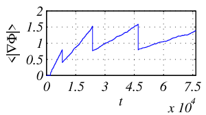
Stabilization of the averaged perturbation gradient $\nabla\Phi=\partial\Phi/\partial\phi$ can also be seen on the left of Fig. 5. Besides the saturation of the gradient the graph illustrates the importance of the number of Fourier modes $K$ involved in the numerical simulation. The jumps in the graph correspond to the instances when we doubled $K$ in order to match the continuously increasing size of the flame. The graph is getting smoother if $K$ is adjusted more gradually and is kept much larger than the ratio of the critical wavelength $\lambda_{cr}=4\pi/\gamma$ to the circumferential length of the flame. The graph on the right of Fig. 5 depicts the energy of the highest order Fourier harmonic involved in the simulation.

According to the data obtained in numerical simulations we may summarize the mechanism of flame front expansion in the Fourier space as follows. The energy of relatively long wave harmonics $\lambda>\lambda_{cr}$ permanently grows according to the Darrieus-Landau instability. This gained energy is transferred towards shorter wavelengths via the nonlinear effects and dissipates through the modes of short enough wavelengths $\lambda<\lambda_{cr}$ . As flame expands the number of short enough angular modes reduces and the overall dissipation rate may become insufficient to counterbalance the generation of energy due to the Darrieus-Landau instability. This results in an accumulation of energy in the short wavelength spectrum, see Fig. 5 (right), and leads to the blow-up of the numerical solution if the number $K$ of used harmonics is not increased in time. This effect explains a slight elevation of the short wave tail of the spectral energy distribution on the right of Fig. 4 in comparison to the graph on the left. The latter one corresponds to the time moment soon after $K$ was doubled, though the former one is just approaching the moment when $K$ needs to be increased.

In general, the process of stabilization of the expanding spherical front to a saturated state is very similar to the planar flame. The only distinctive difference is that the transitional period for the expanding flame is much longer. Using the realistic set of dimensional parameters from [5], e.g. planar flame speed relative to the burnt gases $u_{b}=0.5~m/sec$ and thermal diffusivity $D_{th}=2.5\times 10^{-5}~m^{2}/sec$ , one may interpret our findings in dimensional terms as follows. First cusps begin to appear on the flame surface for $<\!\!r\!\!>\ \approx 0.1~m$ ; flame acceleration with the rate $<\!\!r\!\!>\ \propto t^{3/2}$ starts for $<\!\!r\!\!>\ \approx 0.4~m$ ; acceleration rate begins to slow down for $<\!\!r\!\!>\ \approx 5~m$ , and the acceleration ceases for $<\!\!r\!\!>\ \approx 20~m$ . Most of experiments summarized in [1] and reported in more recent works [15, 16] were carried out in enclosures and were affected by essential pressure rise and acoustics. Thus, there might be a considerable discrepancy between the characteristic flame radii just reported and those measured in realistic combustion experiments. Eventually, of course there is a chance that the stabilization of the expansion rate is just a consequence of the perturbative nature of the governing model used in this work.

4.2 Effect of forcing

A random point-wise set of perturbations uniformly distributed in time and in the Fourier space is a suitable model for both the computational round-off errors and a variety of perturbations of physical origins. In general, such a model would look like

f(x,t)=\sum\limits_{m=1}^{M(t)}a_{m}\cos(\xi_{m}\phi+\varphi_{m})\delta(t-t_{m}),

(31)

where $a_{m}$ , $t_{m}$ , $\xi_{m}$ , and $\varphi_{m}$ are non-correlated random sequences. It is assumed that $t_{1}\leq t_{2}\leq\cdots\leq t_{m}\leq\cdots\leq t_{M(t)}\leq t$ , $0\leq\varphi_{m}\leq 2\pi$ , and $\xi_{m}\geq 0$ , $m=1,2,\ldots,M(t)$ . However, in practice we use only two harmonics with $\xi=\xi_{*}=\floor\left[\gamma\!<\!\!r\!\!>\!\!/2\right]$ and $\xi=\xi_{*}+1$ weighted according to their closeness to the critical wavenumber $\xi_{cr}=\gamma\!<\!\!r\!\!>\!\!/2$ :

f(x,t)\approx f_{0}[(1-\xi_{cr}+\xi_{*})\cos\xi_{*}\phi+(\xi_{cr}-\xi_{*})\cos(\xi_{*}+1)\phi]\sum\limits_{m=0}^{\infty}\delta(t-t_{m}).

(32)

These two harmonics approximate the critical planar flame harmonic of the wavelength $\lambda_{cr}=4\pi/\gamma$ , which was shown to contribute the most in the fastest growing perturbations in the Sivashinsky-type models of flame dynamics, see [17].

The sign of the noise amplitude $f_{0}$ in (32) was either plus or minus for every $m$ with the probability $1/2$ . The delta function $\delta(t-t_{m})$ was approximated by $(\pi\tau)^{-1/2}e^{-(t-t_{m})^{2}/\tau}$ with a small enough value of $\tau$ . The impulse-like noise (32) is used here for the sake of simplicity. Some arguments towards its validity were suggested in [18]. Validation of models like (31), (32) and of the present numerical approach was carried out in [17]. More sophisticated and physically realistic models of temporal noise characteristics can be used with (1) as well.

The importance of the effect of the amplitude of noise and frequency of appearance of the impulse-like perturbations on the flame speed is illustrated in Fig. 6.

More details of the effect of noise are presented in Fig. 7. On the left we plotted graphs of the time instance at which the flame begins to accelerate versus frequency of appearance of the impulse-like perturbations for a variety of the perturbation amplitude $f_{0}$ . Similar graphs of the nearly saturated flame expansion speed are given on the right.

4.3 Three-dimensional numerical experiments

In order to integrate (8)-(10) we used an algorithm which is very similar to that one developed in [9]. In addition, we parallelized the algorithm and used a few techniques to improve its stability and accuracy, see [19].

The basis functions in the spherical harmonics transformation (SHT) are the orthonormal eigenfunctions of the Laplace operator in spherical coordinates. However, unlike the Discrete Fourier Transformation (DFT), the discrete SHT of a data set is its approximation rather than an equivalent representation. Namely, it links a full matrix with $N^{2}$ elements representing a function on a regular spherical mesh of $N^{2}$ nodes in physical space and a triangular matrix of $N^{2}/2$ spherical harmonics coefficients. Thus, every back/forward cycle results in loss of information. This loss is similar to the effect of a short wave filter. In our approach it is associated with the nonlinear term only.

Coordinate singularities at the sphere poles result in accumulation of approximation errors near the poles and weaken numerical stability. In order to prevent accumulation of approximation errors near the poles, we rotate the coordinate system around an axis in the equatorial plane by an angle $\omega$ from time to time. The coordinate transformation formulas for such an axis passing through the points $\phi=\pm\pi/2$ are

\cos\theta^{\prime}=\cos\theta\cos\omega+\sin\theta\sin\omega\cos\phi

\cot\phi^{\prime}=\cot\phi\cos\omega-\csc\phi\sin\omega\cot\theta

Their structure precludes use of the addition theorem for spherical polynomials to transform the coefficients $\widetilde{\Phi}_{n,m}$ to the new coordinate system without the global SHT back to the physical space. On the other hand, the back/forward SHT entails the application of a short wave filter to the whole solution $\widetilde{\Phi}_{n,m}$ , rather than just to the nonlinear term $\widetilde{N}_{n,m}$ . Hence, these rotations should not be done too frequently. Also, it is useful to combine them with rotations around the axis passing through the poles. Implementation of the latter ones is trivial.

Message Passing Interface (MPI) parallelization paradigm was implemented to allow the computational work to be distributed to a number of processors. However, the distributed data needs to be exchanged between these processors, which creates the biggest problem in modelling dynamics of large radius flames. Unlike the multidimensional DFT, discrete SHT does not possess a structure of a tensor product of one-dimensional transformations. Therefore, the data transmission required by the truly distributed discrete SHT is much more sophisticated and intensive than just back/forward row/column transposition of the global solution array required by the DFT, see e.g. [20]. This results in a very fast growth of the communication overheads when the number of processors increases.

Spherical computational algorithms based on parallel Legendre-Fourier transformations are much less efficient than the standard planar Fourier methods. However, expanding spherical flames can be successfully simulated by the parallel SFT method. An example of the evolution of a random three-dimensional perturbation of a spherical flame is illustrated in Fig. 8.

4.4 Dynamics of curved flame segments

Our numerical experiments showed that long time simulations of the three-dimensional expanding flames using discrete SHT might be possible on a parallel computer with large enough physically shared memory. However, there is an alternative approach based on simulations of the three-dimensional flame segments and following extension to the whole surface by periodicity. In order to validate this idea we applied it to the two-dimensional flames first.

Results of two-dimensional numerical simulations of the dynamics of sectors $\theta\in[0,2\pi/\theta_{\pi}]$ of a spherical flame are illustrated in Fig. 9. One may see that the narrowing of the sector does not affect the flame expansion rate in absence of explicit forcing and that a correlation between this rate and the size of the segment becomes apparent as forcing strengthens. Similar observations were obtained for other parameters discussed earlier in this Section.

Our calculations also show that there is a critical value of $\theta_{\pi}$ above which sectorial simulations no longer represent the whole spherical flame. For example, we would not present the results of our simulations with $\theta_{\pi}=16$ as an approximation for the whole spherical flame. However, based on our two-dimensional results, it looks like simulations of the three-dimensional spherical flames using the Fourier, rather than the Fourier-Legendre, spectral model of the Sivashinsky type in the sector $0\leq\theta,\phi\leq\pi$ , or even in $0\leq\theta,\phi\leq\pi/2$ , are safe.

5 Conclusions

Long time interval simulations of a simplified model of the expanding spherical flames indicated that their expansion rate slows down as the flame size grows. The saturation of the planar flame propagation speed as their size grows was established too. Hence, a hypothesis of stabilization of the spherical flame expansion rate over a finite time interval is proposed.

Further similarities with the propagating planar flames achieved by the expanding spherical flames on large time intervals were established in the studies of the effect of forcing, revealing a clear correlation between the strength of the forcing and the flame expansion rate. This supports the idea that the acceleration of both planar and expanding flames results from explicit and/or implicit forcing, which is always present both in experiments and calculations at least as noise of various physical origins.

In spite of many benefits of the simplified flame dynamics models, they have not been constructed to cope with significant perturbations of spherical flames. This casts a reasonable doubt in the possibility of extending the effects observed for the simplified model to realistic flames. In order to verify the hypothesis, numerical simulations of a more sophisticated model are required. In particular, model [8] is valid for flames of any geometry if thermal gas expansion due to combustion does not generate significant vorticity, i.e. for $\gamma\ll 1$ . However, even in the coordinate form (3)-(6) the governing equation of model [8] is extremely difficult to solve numerically, because, in contrast to (2), its nonlocal term has no convolution structure.

Using parallelized spherical harmonics transformation, the evolution of a three-dimensional expanding spherical flame has been successfully simulated to a stage when wrinkles appear and form a well developed cellular structure. However, computational problems associated with the spherical harmonics transformation make it difficult to extend these calculations on time intervals which would match those attained in our two-dimensional simulations. On the other hand, it was also noticed that the simulations of the three-dimensional spherical flames using the Fourier, rather than the Fourier-Legendre, spectral model of the Sivashinsky type in the sector $0\leq\theta,\phi\leq\pi$ , or even in $0\leq\theta,\phi\leq\pi/2$ , are reasonable.

Acknowledgements

This work was supported by the EPSRC (Grant GR/R66692, UK), the US-Israel Binational Science Foundation (Grant 200 2008), the German-Israel Foundation (Grant G-695-15.10/2001), and the Israel Science Foundation (Grants 67-01 and 278-03). One of the authors is grateful to the Royal Society, The Academy Study Group on Israel and the Middle East, and to the Tel Aviv University for their support when working on this paper.

References

[1] Y.A. Gostintsev, A.G. Istratov, and Y.V. Shulenin. A self-similar regime of free turbulent flame propagation in mixed gaseous mixtures. Physics of Combustion and Explosion, 24(5):63–70, 1988.
[2] A.G. Istratov and V.B. Librovich. On the stability of gasdynamic discontinuities associated with chemical reactions. The case of a spherical flame. Acta Astronautica, 14:453–467, 1969.
[3] J.K. Bechtold and M. Matalon. Hydrodynamic and diffusion effects on the stability of spherically expanding flames. Combustion and Flame, 67:77–90, 1987.
[4] G.I. Sivashinsky. Nonlinear analysis of hydrodynamic instability in laminar flames - I. Derivation of basic equations. Acta Astronautica, 4:1177–1206, 1977.
[5] L. Filyand, G.I. Sivashinsky, and M.L. Frankel. On self-acceleration of outward propagating wrinkled flames. Physica D, 72:110–118, 1994.
[6] G. Joulin. Nonlinear hydrodynamic instability of expanding flames: Intrinsic dynamics. Physical Review E, 50(3):2030–2047, 1994.
[7] O. Thual, U. Frisch, and M. Hénon. Application of pole decomposition to an equation governing the dynamics of wrinkled flame fronts. Le Journal de Physique, 46(9):1485–1494, Septembre 1985.
[8] M.L. Frankel. An equation of surface dynamics modeling flame fronts as density discontinuities in potential flows. Phys. Fluids A, 2(10):1879–1883, 1990.
[9] Y. D’Angelo, G. Joulin, and G. Boury. On model evolution equations for the whole surface of three-dimensional expanding wrinkled premixed flames. Combustion Theory and Modelling, 4:1–22, 2000.
[10] http://www.scd.ucar.edu/css/software/spherepack. Spherepack 3.0. University Corporation for Atmospheric Research.
[11] V. Karlin. Cellular flames may exhibit a nonmodal transient instability. Proceedings of the Combustion Institute, 29(2):1537–1542, 2002.
[12] G. Joulin. On the hydrodynamic stability of curved premixed flames. J. Phys. France, 50:1069–1082, Mai 1989.
[13] V. Karlin. Nonmodal instability as the mechanism of acceleration of cellular flames. In A.B. Movchan, editor, IUTAM Symposium on Asymptotics, Singularities and Homogenization in Problems of Mechanics, pages 549–556. Kluwer Academic Publishers, 2003.
[14] V. Karlin. Estimation of the linear transient growth of perturbations of cellular flames. 14(8):1191–1210, 2004.
[15] D. Bradley, R.A. Hicks, M. Lawes, C.G.W. Sheppard, and R. Woolley. The measurement of laminar burning velocities and Markstein numbers for iso-octane-air and iso-octane- $n$ -heptane-air mixtures at elevated temperatures and pressures in an explosion bomb. Combustion and Flame, 115:126–144, 1998.
[16] G. Rozenchan, D. L. Zhu, C. K. Law, and S. D. Tse. Outward propagation, burning velocities, and chemical effects of methane flames up to 60 atm. Proceedings of the Combustion Institute, 29(2):14611469, 2002.
[17] V. Karlin. Detailed analysis of a pseudoresonant interaction between cellular flames and velocity turbulence. Preprint arXiv:physics/0502036, at http://arxiv.org, February 2005. 20 pp.
[18] G. Joulin. On a model for the response of unstable premixed flames to turbulence. Combustion Science and Technology, 60:1–5, 1988.
[19] J. Mai and V. Karlin. Numerical study of premixed laminar spherical flames. In Proceedings of the European Combustion Meeting (ECM 2005), Louvain-la-Neuve, Belgium, April 3–6 2005. paper 090.
[20] V. Karlin, V. Maz’ya, and G. Schmidt. High accuracy periodic solutions to the Sivashinsky equation. Journal of Computational Physics, 188(1):209–231, 2003.