Kinetic theory models for the distribution of wealth: power law from overlap of exponentials

In the first version of the model, so far unnoticed in later literature, the money difference $\Delta x$ is assumed to have a constant value Bennati1988a; Bennati1988b; Bennati1993a,

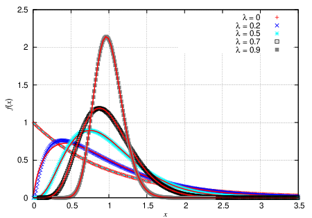
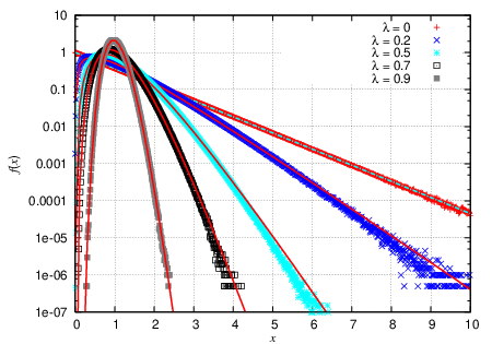
This rule, together with the constraint that transactions can take place only if $x_{i}^{\prime}>0$ and $x_{j}^{\prime}>0$, provides a Boltzmann distribution; see the curve for $\lambda=0$ in Fig. 1. An equilibrium distribution with exponential tail is also obtained if $\Delta x$ is a random fraction $\epsilon$ of the wealth of one of the two agents, $\Delta x=\epsilon x_{i}$ or $\Delta x=\epsilon x_{j}$. A trading rule based on the random redistribution of the sum of the wealths of the two agents has been introduced by Dragulescu and Yakovenko Dragulescu2000a,

where $\epsilon$ is a random number uniformly distributed between 0 and 1 and $\bar{\epsilon}$ is the complementary fraction, i.e. $\epsilon+\bar{\epsilon}=1$. Equations (3) are easily shown to correspond to the trading rule (1), with

In the following we will concentrate on the latter version of the model and its generalizations, though both the versions of the basic model defined by Eqs. (2) or (4) lead to the Boltzmann distribution,

where the effective temperature of the system is just the average wealth $\left\langle x\right\rangle$ Bennati1988a; Bennati1988b; Bennati1993a; Dragulescu2000a. The result (5) is found to be robust, in that it is largely independent of various factors. Namely, it is obtained for the various forms of $\Delta x$ mentioned above, for pairwise as well as multi-agent interactions, for arbitrary initial conditions Chakraborti2000a, and finally, for random or consecutive extraction of the interacting agents. The Boltzmann distribution thus obtained has been sometimes referred to as an “unfair distribution”, in that it is characterized by a majority of poor agents and very few rich agents, as signaled in particular by a zero mode and by the exponential tail. The form of distribution (5) will be referred to as the Boltzmann distribution and is also known as Gibbs distribution.

Despite the Boltzmann distribution is robust respect to the variation of several parameters, the way it depends on the details of the trading rule is subtle. For instance, in the model studied in Ref. Chakraborti2002a, the equilibrium distribution can have a very different shape. In that model it is assumed that both economic agents $i$ and $j$ invest the same amount $x_{min}$, which is taken as the minimum wealth of the two agents, $x_{min}={\mathrm{min}}\{x_{i},x_{j}\}$. The wealths after the trade are $x_{i}^{\prime}=x_{i}+\Delta x$ and $x_{j}^{\prime}=x_{j}-\Delta x$, where $\Delta x=(2\epsilon-1)x_{min}$.

We note that once an agent has lost all his wealth, he is unable to trade because $x_{min}$ has become zero. Thus, a trader is effectively driven out of the market once he loses all his wealth. In this way, after a sufficient number of transactions only one trader survives in the market with the entire amount of wealth, whereas the rest of the traders have zero wealth.

A step toward generalizing the basic model and making it more realistic is the introduction of a saving criterion regulating the trading dynamics. This can be achieved defining a saving propensity $0<\lambda<1$, that represents the fraction of wealth saved — and not reshuffled — during a transaction. The dynamics of the model is as follows Chakraborti2000a; Chakraborti2002a:

with $\bar{\epsilon}=1-\epsilon$, corresponding to a $\Delta x$ in Eq. (1) given by

This model leads to a qualitatively different equilibrium distribution. In particular, it has a mode $x_{m}>0$ and a zero limit for small $x$, i.e. $f(x\!\to 0)\!\to 0$, see Fig. 1. The functional form of such a distribution has been conjectured to be a Gamma distribution on the base of an analogy with the kinetic theory of gases, which is consistent with the excellent fitting provided to numerical data Patriarca2004b; Patriarca2004c. Its form can be conveniently written by defining the effective dimension $D_{\lambda}$ as Patriarca2004c

According to the equipartition theorem, one can introduce a corresponding temperature defined by the relation $\left\langle x\right\rangle={D_{\lambda}}T_{\lambda}/2$, i.e.

Then the distribution for the reduced variable $\xi=x/T_{\lambda}$ reads

i.e. a Gamma distribution of order $D_{\lambda}/2$. For integer or half-integer values of $n=D_{\lambda}/2$, this function is identical to the equilibrium Maxwell-Boltzmann distribution of the kinetic energy for a system of molecules in thermal equilibrium at temperature $T_{\lambda}$ in a $D_{\lambda}$-dimensional space (see Appendix A for a detailed derivation). For $D_{\lambda}=2$, the Gamma distribution reduces to the Boltzmann distribution. This extension of the equivalence between kinetic theory and closed economy models to values $0\leq\lambda<1$ is summarized in Table 1.

This equivalence between a multi-agent system with a saving propensity $0\leq\lambda<1$ and an $N$-particle system in a space with effective dimension $D_{\lambda}\geq 2$ was originally suggested by simple considerations about the kinetics of a collision between two molecules. In fact, for kinematical reasons during such an event only a fraction of the total kinetic energy can be exchanged. Such a fraction is of the order of $1-\lambda\approx 1/D$, to be compared with the expression $1-\lambda=3/(D/2+2)$ derived from Eq. (8) Patriarca2004c.

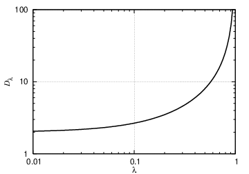
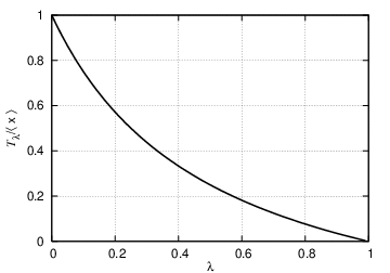
While $\lambda$ varies between 0 and 1, the parameter $D_{\lambda}$ monotonously increases from 2 to $\infty$, and the effective temperature $T_{\lambda}$ correspondingly decreases from $\left\langle x\right\rangle$ to zero; see Fig. 2. It is to be noticed that according to the equipartition theorem only in $D_{\lambda}=2$ effective dimensions ($\lambda=0$) the temperature coincides with the average value $\left\langle x\right\rangle$, $T_{\lambda}=2\left\langle x\right\rangle/2\equiv\left\langle x\right\rangle$, as originally found in the basic model Bennati1988a; Bennati1988b; Bennati1993a; Dragulescu2000a. In its general meaning, temperature represents rather an estimate of the fluctuation of the quantity $x$ around its average value. The equipartition theorem always gives a temperature smaller than the average value $\left\langle x\right\rangle$ for a number of dimensions larger than two. In the present case, Eqs. (8) or (9) show that this happens for any $\lambda>0$.

The dependence of the fluctuations of the quantity $x$ on the saving propensity $\lambda$ was studied in Ref. Chakraborti2000a. In particular, the decrease in the amplitude of the fluctuations with increasing $\lambda$ is shown in Fig. 3.

The fact that in general the market temperature $T_{\lambda}$ decreases with $\lambda$ means smaller fluctuations of $x$ during trades, consistently with the saving criterion, i.e. with a $\lambda>0$. One can notice that in fact $T_{\lambda}=(1-\lambda)\left\langle x\right\rangle/(1+2\lambda)\approx(1-\lambda)\left\langle x\right\rangle$ is of the order of the average amount of wealth exchanged during a single interaction between agents, see Eqs. (6).

In order to take into account the natural diversity between various agents, a model with individual propensities $\{\lambda_{i}\}$ as quenched random variables was studied in Refs. Chatterjee2003a; Chatterjee2004a. The dynamics of this model is the following:

where, as above, $\bar{\epsilon}=1-\epsilon$. This corresponds to a $\Delta x$ in Eq. (1) given by

Besides the use of this trading rule, a further prescription is given in the model, namely an average over the initial random assignment of the individual saving propensities: With a given configuration $\{\lambda_{i}\}$, the system is evolved until equilibrium is reached, then a new set of random saving propensities $\{\lambda_{i}^{\prime}\}$ is extracted and reassigned to all agents, and the whole procedure is repeated many times. As a result of the average over the equilibrium distributions corresponding to the various $\{\lambda_{i}\}$ configurations, one obtains a distribution with a power law tail, $f(x)\propto x^{-\alpha-1}$, where the Pareto exponent has the value $\alpha=1$. This value of the exponent has been predicted by various theoretical approaches to the modeling of multi-agent systems Das2003a; Repetowicz2004a; Chatterjee2005a.

A key point which explains many of the features of the model and of the corresponding equilibrium state is a well-defined correlation between average wealth and saving propensity, which has been unnoticed so far in the literature Manna_here. The existence of such a correlation can be related to the origin of the power law and its cut-off at high values of $x$. It also explains the paradox according to which a very rich agent may lose all his wealth when interacting with poor agents, as a consequence of the stochastic character of the trading rule defined by Eq. (11).

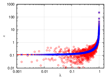
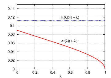
Figure 4 shows the equilibrium state for a system with $N=1000$ agents after $t=10^{9}$ trades. Each agent is represented by a circle ($\circ$) in the wealth-saving propensity $x_{i}$-$\lambda_{i}$ plane. The correlation between wealth $x$ and saving propensity $\lambda$ becomes very high at large values of $x$ and $\lambda$. Namely, one observes that the average wealth $\left\langle x(\lambda)\right\rangle$ [crosses ($\times$) in Fig. 4] diverges for $\lambda\to 1$. The average $\left\langle x(\lambda)\right\rangle$ was obtained by computing the probability density $f(x,\lambda)$ in the $x$-$\lambda$ plane (normalized so that $\int dx\,d\lambda\,f(x,\lambda)=1$) and averaging for a fixed value of $\lambda$,

The observed correlation naturally follows from the structure of the trade dynamics (11). We remind that initially every agent has the same wealth $x_{0}=\left\langle x\right\rangle$. During the initial phase of the evolution, when all agents have approximately the same wealth $\left\langle x\right\rangle$, an agent $i$ with a large saving propensity $\lambda_{i}$ can save more — on average — and therefore accumulate more. Afterwards, the agent $i$ will continue to enter trades by investing only a small fraction $(1-\lambda_{i})x_{i}$ of his wealth $x_{i}$ in the trade. Even when interacting with an agent $j$, with a smaller wealth $x_{j}<x_{i}$, agent $i$ may still be successful in the trading, since agent $j$ may have also a smaller saving propensity $\lambda_{j}$, so that the traded fraction of wealth $(1-\lambda_{j})x_{j}$ is comparable with or even larger than $(1-\lambda_{i})x_{i}$. Trading by agent $i$ will very probably be successful on average with all agents $j$ with a $\lambda_{j}$ such that $(1-\lambda_{j})x_{j}$ is smaller than $(1-\lambda_{i})x_{i}$. These considerations suggest that agent $i$ will reach equilibrium (and his maximum possible wealth) when $(1-\lambda_{i})x_{i}=\kappa\approx\left\langle(1-\lambda)x\right\rangle$. The ratio between the constant $\kappa$ and the average $\left\langle(1-\lambda)x\right\rangle=\sum_{j}(1-\lambda_{j})x_{j}/N$ is actually found to be of the order of magnitude of 10. The formula

however, shown as a continuous line in Fig. 4, provides an excellent interpolation of the average wealth $\left\langle x(\lambda)\right\rangle$ (also shown in the figure) computed numerically.

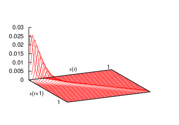
The stability of the asymptotic state is also shown by the histogram in Fig. 5 of the wealths $x^{\prime}\equiv x(t+1)$ after a trade versus $x\equiv x(t)$ before it defined in Eqs. (1). The distribution is narrower at larger values of $x$ than at smaller ones, implying that the probability that an agent $i$ will undergo a large relative variation of his wealth $x_{i}$ within a single trade is much higher for poor agents. The situation at small $x$ (corresponding to agents with smaller saving propensities) is instead more similar to that of the trading rule without saving ($\lambda=0$), Eqs. (6): the distribution is broader, indicating a higher probability of a large wealth reshuffling during a trade.

A peculiarity of the model with individual saving propensities is noteworthy. On one hand, in the procedure used to obtain a power law in Ref. Chatterjee2003a all agents are equivalent to each other: they enter the dynamical evolution law on an equal footing, their saving propensities are reassigned randomly with the same uniform distribution between 0 and 1, and even their initial conditions can be set to be all equal to each other, $x_{i}=\left\langle x\right\rangle$, without loss of generality. Therefore the various equilibrium configurations, corresponding to different sets $\{\lambda_{i}\}$, are expected to be statistically equivalent to each other, in the sense that one should be able to obtain the power law distribution by a simple ensemble average for any fixed configuration of saving propensities $\{\lambda_{i}\}$, if the number of agents $N$ is large enough. On the other hand, an averaging procedure over several $\{\lambda_{i}\}$ configurations is in practice necessary to obtain a power law distribution.

In order to understand this apparent paradox, we checked how the equilibrium distributions, corresponding to a given set of saving propensities $\{\lambda_{i}\}$, look like. One finds that every configuration $\{\lambda_{i}\}$ produces equilibrium distributions very different from each other; see Fig. 6 for some examples. The structures observed are very different from power laws, with well resolved peaks at large $x$. Only when an average over different $\{\lambda_{i}\}$ configurations is carried out, one obtains a smooth power law with Pareto exponent $\alpha=1$.

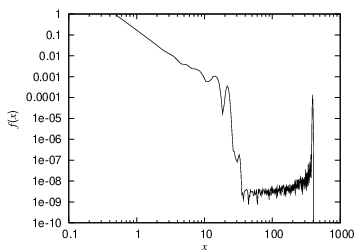
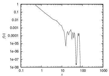
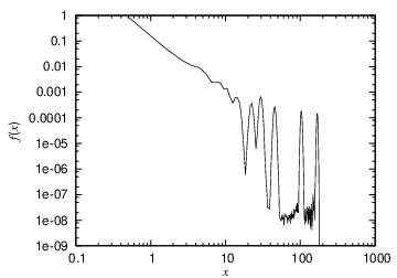
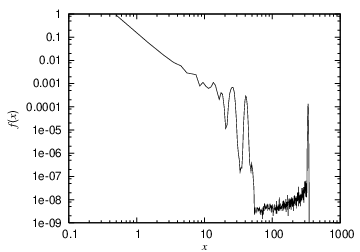
These same figures show, however, that for a given configuration $\{\lambda_{i}\}$ a power law is actually observed at small values of $x$. Another related interesting feature of simulations employing a single saving propensity configuration $\{\lambda_{i}\}$ is that a power law distribution is found only on a limited time scale, while it disappears partly or totally at equilibrium. Thus also in the time dimension one surprisingly finds a distribution much more similar to a power law at a smaller rather than larger scale.

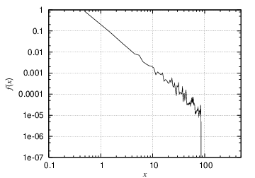
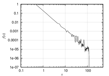
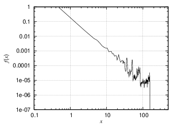
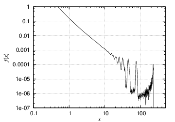
This is shown in the example in Fig. 7, where the distributions of a system of 1000 agents at four different times are compared to each other. These features suggest that the power law is intrinsically built into the dynamical laws of the model but that, for some reasons, it fades away at large $x$ and $t$ scales. The $x$-$\lambda$ correlation discussed above in Sec. 3.1 can provide an explanation of these features, both for those in the $x$ and in the time dimension, as discussed below.

The peculiar features illustrated above, the necessity of averaging over different configurations $\{\lambda_{i}\}$ as done in Ref. Chatterjee2003a to obtain a power law distribution, as well as the power law distribution itself, are here explained in terms of equilibrium states of suitably defined subsystems and the $x$-$\lambda$ correlation illustrated above. This may seem odd since at first sight the averaging procedure of Ref. Chatterjee2003a defines a nonequilibrium process, the system being brought out of equilibrium from time to time by the reassignment of the saving propensities. Correspondingly, one may attribute the power law to the underlying dynamical process, as it is often the case in nonequilibrium models (e.g. models of markets on networks Chatterjee_here).

However, if one considers the partial distributions of agents with a certain value of $\lambda$, one finds an unexpected result. For numerical reasons we consider the subsets made up of those agents with saving propensity $\lambda$ within a window $\Delta\lambda$ around a given value $\lambda$. Figure 8 (upper row) shows the partial distributions (continuous lines) of the ten subsystems obtained by dividing the $\lambda$ range (0,1) into ten slices of width $\Delta\lambda=0.1$ and average values 0.05,$\dots$,0.95 (curves from left to right respectively). Most of the partial distributions have an exponential tail, and only when summed up their overlap (dotted line) reproduces a power law.

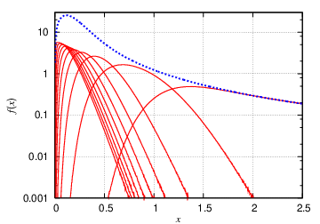
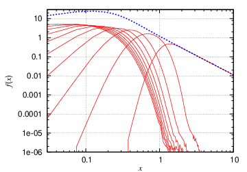
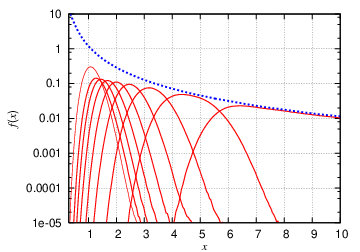
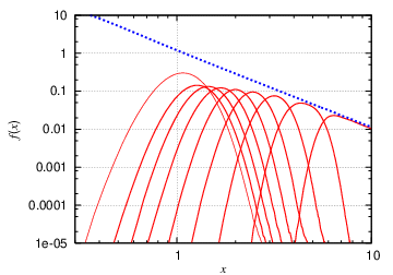
It can be noticed that the last partial distribution, corresponding to the interval $\lambda=(0.9,1.0)$, is not of exponential form, but rather presents a power law tail, which overlaps with the total distribution at large $x$. However, its power law form is due only to the low resolution in $\lambda$ employed. In fact even this partial distribution can in turn be shown to be given by the superposition of exponential tails. By increasing the resolution in $\lambda$, i.e. using a smaller interval $\Delta\lambda=0.01$ to further resolve the interval $\lambda=(0.9,1.0)$ into subintervals with average values $\lambda=0.905,\dots,0.995$, one obtains the partial distributions shown in the lower row of Fig. 8. It is to be noticed that also in this case the last partial distribution corresponding to the interval $\lambda=(0.99,1.00)$ has a power law tail. The procedure can then in principle be reiterated to resolve also this partial distribution by increasing the resolution in $\lambda$.

These facts also explain the origin of the peaks visible at large $x$ in the plots in Figs. 6 and 7. Due to the high wealth-saving propensity correlation at large values of $x$, see Fig. 4, these peaks are due to agents with high $\lambda$. The reason why these agents give rise to resolved peaks instead of contributing to extending the power law tail is that the partial distributions (i.e. the average values) of single agents get farther and farther from each other for $\lambda\to 1$, while the corresponding widths do not grow enough to ensure the overlap of the distributions of neighbor agents in $\lambda$-space. Eventually, each agent (or cluster of agents) at high values of $x$ will be resolved as an isolated peak against the background of the total distribution. In greater detail, one finds that the average value $\left\langle x(\lambda)\right\rangle$ diverges for $\lambda\to 1$ as $1/(1-\lambda)$, as shown in Fig. 4. This implies that also the distance between two generic consecutive agents increases: if agents are labeled from $i=1$ to $i=N$ in order of increasing $\lambda$ ($\lambda_{1}<\dots<\lambda_{N}$) and the $\lambda$ distribution is uniform, then $\Delta\lambda=\lambda_{i+1}-\lambda_{i}={\mathrm{constant}}$. The distance between the average positions of the partial distributions of two consecutive agents is, from Eq. (14),

where $\kappa$ is a constant. Thus $\delta\!\left\langle x(\lambda)\right\rangle$ diverges even faster than $\left\langle x(\lambda)\right\rangle$. At the same time, the width of the partial distribution $\Delta x(\lambda)$, here estimated as $\Delta x(\lambda)=\sqrt{\left\langle x^{2}(\lambda)\right\rangle-\left\langle x(\lambda)\right\rangle^{2}}$, grows slower than $\left\langle x(\lambda)\right\rangle$, i.e. for $\lambda\to 1$ the ratio $\Delta x(\lambda)/\left\langle x(\lambda)\right\rangle\to 0$; see Fig. 4 (right). The breaking of the power law and the appearance of the isolated peaks takes place at a cutoff $x_{c}$ where the distance $\delta\!\left\langle x(\lambda)\right\rangle$ between the peaks corresponding to consecutive agents $i$ and $i+1$ becomes comparable with the peak width $\Delta x(\lambda)$.

Also the origin of the peculiarities in the time evolution of the distribution function, mentioned in Sec. 3.3, can now be explained easily. In order to reach the asymptotic equilibrium state, agents can rely on an income flux which is on average proportional to $x_{i}(1-\lambda_{i})$. At the beginning, when all agents have the same wealth $x_{i}=x_{0}$, this quantity is smaller for agents with a larger $\lambda_{i}$; and with this smaller flux agents with large $\lambda_{i}$ have to reach their higher asymptotic value $\propto 1/(1-\lambda_{i})$. As a consequence, the relaxation time of an agent is larger for larger $\lambda$, a result already found in the numerical simulations of the multi-agent model with fixed global saving propensity (see Fig. 2 in Ref. Chakraborti2000a). Correspondingly, partial distributions of rich agents will reach their asymptotic form later (last frame in Fig. 7), while, at intermediate times, their distributions will be spread at smaller values of $x$, contributing to smoothen the total distribution (first frame in Fig. 7).

It is also possible to explain why the averaging procedure of Ref. Chatterjee2003a is successful in producing a power law distribution. Averaging over different configurations $\{\lambda_{i}\}$ is equivalent to simulate a very dense distribution in $\lambda$ — which has large relaxation time and number of agents — with an affordable number of agents and computer time. However, the procedure is not needed in principle, since the power law can be obtained also when a single configuration with a proper density in $\lambda$-space is used.

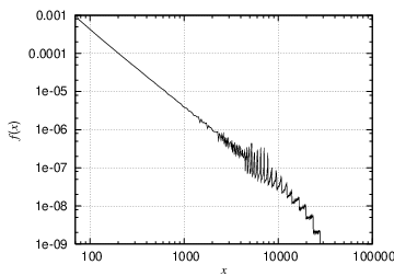
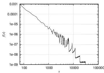
A practical way to avoid the appearance of the peaks at large $x$ and obtain a distribution closer to a power law is to increase the density of agents, especially at values of $\lambda$ close to 1. In a random extraction of $\{\lambda_{i}\}$, it is natural that consecutive values of $\lambda_{i}$ will not be equally spaced. Even small differences will be amplified at large $x$ and will result in the appearance of peaks. A deterministic assignment of the $\lambda$, e.g. a uniform distribution achieved through the following assignment,

is a uniform distribution of $\lambda$ in the interval [0,1) and will generate a smoother distribution of $x$. The comparison of the results for this distribution with those for a random distribution of $\lambda$ is done in Fig. 9 (notice the high value of $N$). In the uniform case not only the power law extends to higher values of $x$ but also that the distribution of peaks at large $x$ is globally smoother, in the sense that on average the single peaks follow a power law better.

References

- (1) Encyclopaedia Britannica, www.britannica.com/ebc/article?tocId=9372448.
- (2) F. Shostak, Quarterly J. Australian Econ. 3 (2000) 69.
- (3) www.answers.com/income&r=67.
- (4) E. Bennati, La simulazione statistica nell’analisi della distribuzione del reddito: modelli realistici e metodo di Montecarlo, ETS Editrice, Pisa, 1988.
- (5) E. Bennati, Un metodo di simulazione statistica nell’analisi della distribuzione del reddito, Rivista Internazionale di Scienze Economiche e commerciali (1988) 735–756.
- (6) E. Bennati, Il metodo di Montecarlo nell’analisi economica, Rassegna di lavori dell’ISCO 10 (1993) 31.
- (7) A. Dragulescu, V. M. Yakovenko, Statistical mechanics of money, Eur. Phys. J. B 17 (2000) 723.
- (8) A. Chakraborti, B. K. Chakrabarti, Statistical mechanics of money: how saving propensity affects its distribution, Eur. Phys. J. B 17 (2000) 167.
- (9) A. Chakraborti, Distributions of money in model markets of economy, Int. J. Mod. Phys. C 13 (2002) 1315.
- (10) A. Chatterjee, B. K. Chakrabarti, S. S. Manna, Money in gas-like markets: Gibbs and Pareto laws, Physica Scripta T106 (2003) 367.
- (11) A. Chatterjee, B. K. Chakrabarti, S. S. Manna, Pareto law in a kinetic model of market with random saving propensity, Physica A 335 (2004) 155.
- (12) A. Chatterjee, B. K. Chakrabarti, R. B. Stinchcombe, Master equation for a kinetic model of trading market and its analytic solution, http://arxiv.org/abs/cond-mat/0501413.
- (13) V. Pareto, Cours d’economie politique, Rouge, Lausanne, 1897.
- (14) M. Patriarca, A. Chakraborti, K. Kaski, Gibbs versus non-Gibbs distributions in money dynamics, Physica A 340 (2004) 334.
- (15) M. Patriarca, A. Chakraborti, K. Kaski, Statistical model with a standard Gamma distribution, Phys. Rev. E 70 (2004) 016104.
- (16) A. Das, S. Yarlagadda, A distribution function analysis of wealth distribution, http://arxiv.org/abs/cond-mat/0310343.
- (17) P. Repetowicz, S. Hutzler, P. Richmond, Dynamics of money and income distributions, http://arxiv.org/abs/cond-mat/0407770.
- (18) See however similar findings of S. S. Manna in this volume.
- (19) See the contribution by A. Chatterjee in this volume.