跳到论文正文
W Papers独立论文阅读器 arXiv:physics/0504112 论文正文 计算阅读时间 · 0%
引用这篇论文根据当前论文元数据生成,正式投稿前建议核对。


License: Assumed arXiv.org perpetual non-exclusive license
arXiv:physics/0504112v3 [physics.optics] 08 Apr 2006

Slow light in photonic crystals

Alex Figotin    Ilya Vitebskiy Affiliation: Department of Mathematics, University of California at Irvine, CA 92697
Abstract

The problem of slowing down light by orders of magnitude has been extensively discussed in the literature. Such a possibility can be useful in a variety of optical and microwave applications. Many qualitatively different approaches have been explored. Here we discuss how this goal can be achieved in linear dispersive media, such as photonic crystals. The existence of slowly propagating electromagnetic waves in photonic crystals is quite obvious and well known. The main problem, though, has been how to convert the input radiation into the slow mode without losing a significant portion of the incident light energy to absorption, reflection, etc. We show that the so-called frozen mode regime offers a unique solution to the above problem. Under the frozen mode regime, the incident light enters the photonic crystal with little reflection and, subsequently, is completely converted into the frozen mode with huge amplitude and almost zero group velocity. The linearity of the above effect allows the slowing of light regardless of its intensity. An additional advantage of photonic crystals over other methods of slowing down light is that photonic crystals can preserve both time and space coherence of the input electromagnetic wave.

1 Introduction

1.1 What is slow light?

It is common knowledge that, in vacuum, light propagates with constant velocity c≈3×10⁸c\approx 3\times 10^{8}m/sec. In optically transparent nondispersive media, the speed of light propagation is different

v=ω/k=c/n,v=\omega/k=c/n, (1)

where kk is the wave number, ω\omega is the respective frequency, and nn is the refractive index of the medium. At optical frequencies, the refractive index nn of transparent materials usually does not exceed several units, and the speed of light propagation is of the same order of magnitude as in vacuum.

The situation can change dramatically in strongly dispersive media. Although the phase velocity of light is still determined by the same expression (1), the speed of electromagnetic pulse propagation is different from vv and is determined by the group velocity [1, 2, 3]

u=∂ω∂k=c​(n+ω​d​nd​ω)−1,u=\frac{\partial\omega}{\partial k}=c\left(n+\omega\frac{dn}{d\omega}\right)^{-1}, (2)

which is one of the most important electromagnetic characteristics of the medium. With certain reservations, the group velocity uu coincides with the electromagnetic energy velocity and is usually referred to simply as the propagation speed of light in the medium. Hereinafter, the speed of light propagation means the group velocity (2), rather then the phase velocity (1).

Strong dispersion means that the group velocity uu strongly depends on the frequency and can be substantially different from cc. In the slow light case, which is the subject of our interest, the electromagnetic pulse propagates through the dispersive medium at the speed u≪cu\ll c, regardless of the respective value of the phase velocity (1). In some cases, uu can even become vanishingly small implying that the propagating electromagnetic mode at the respective frequency does not transfer energy. In another extreme case, the group velocity uu can exceed cc (the so-called case of superluminal pulse propagation), without contradicting the causality principle [1, 4, 5, 6, 7]. In yet another case of a left-handed medium, the group velocity uu can have the opposite sign to that of the phase velocity vv [8]. But again, in this paper we will focus exclusively on the slow light and related phenomena.

Slow and ultraslow light have numerous and diverse practical applications. The related phenomena include dramatic enhancement of various light-matter interactions such as nonlinear effects (higher harmonic generation, wave mixing, etc.), magnetic Faraday rotation, as well as many other important electromagnetic properties of the optical media. Such an enhancement can facilitate design of controllable optical delay lines, phase shifters, miniature and efficient optical amplifiers and lasers, etc. In addition, ultraslow light might allow nonlinear interactions down to a single photon level, which could significantly benefit the design of ultrasensitive optical switches, quantum all-optical data storage and data processing devices. Ultraslow light can also be used in quantum communication and design of novel acousto-optical devices. This list can be continued. For more detailed information on the prospective practical applications of slow light phenomena see, for example, [9, 10, 11, 12, 13, 14, 15, 16, 17, 18, 19, 20, 21, 22, 23, 24, 25, 26, 27, 28, 29, 30, 33] and references therein.

1.2 Temporal dispersion versus spatial dispersion

In recent years, several different approaches have been pursued in order to slow down or even completely stop light. These approaches can be grouped into two major categories:

  • -

    those where the low group velocity results from strong temporal dispersion d​n/d​ωdn/d\omega of optical media;

  • -

    those where the low speed of pulse propagation is a result of coherent interference in spatially periodic heterogeneous media, such as photonic crystals.

Let us start with a brief discussion of slow light phenomena in media with strong temporal dispersion.

1.2.1 Slow light in media with strong temporal dispersion

Assuming that the refractive index nn in (2) is of the order of unity, which is usually the case at optical frequencies, one can state that a very low group velocity can only occur if nn varies strongly as a function of ω\omega

u≈c​(ω​d​nd​ω)−1≪c​ only if ​ω​d​nd​ω≫1.u\approx c\left(\omega\frac{dn}{d\omega}\right)^{-1}\ll c\text{ \ only if }\omega\frac{dn}{d\omega}\gg 1. (3)

Strong frequency dependence of the refractive index nn can be a result of excitation of electronic or some other intrinsic resonances of the medium, which are normally accompanied by strong absorption of light. Recently, though, several techniques have been developed that allow to significantly suppress the absorption of light at the frequency where the derivative d​n/d​ωdn/d\omega peaks.

One of the most successful ways to suppress light absorption is based on the effect of electromagnetically induced transparency (EIT) [35]. In such a case, the incident light interacts with atomic spin excitations forming combined excitations of photons and spins, called dark-state polaritons. These polaritons propagate slowly through the medium in the form of a sharply compressed pulse, the energy of which is much smaller than that of the incident light pulse. Most of the incident light energy is expended to create the coherent state of the atomic spins, the rest is carried away by the control electromagnetic field. The pulse delay inside the medium is limited by the bandwidth of the transparency window, which decreases with propagation distance. At higher propagation distances the medium becomes increasingly opaque at frequencies other than the line center, further reducing the available transparency window [12, 13]. Specific physical mechanisms of such transformations are very diverse. The detailed description of EIT and related phenomena can be found in the extensive literature on the subject (see, for example, [9, 10, 11, 12, 13, 14], and references therein). The techniques based on EIT have already produced some amazing results, such as reduction of the speed of pulse propagation by 7 – 8 orders of magnitude compared to the speed of light in vacuum, while providing a huge and controllable pulse delay.

Another method to create a transparency window in otherwise opaque substance was used in [15, 16]. This method involves the creation of a spectral hole by the periodic modulation of the ground state population at the beat frequency between the pump and the probe fields applied to the material sample. It can produce slow light in a solid-state material at room temperature. The spectral hole created by this technique can be extremely narrow (36 Hz in the experiment [15, 16]), and leads to a rapid spectral variation of refractive index. It allowed to reduce the light group velocity in a ruby crystal down to 57 m/s.

Physically, the above approaches to slowing down the light can be viewed as a reversible transformation of the input nearly monochromatic light into some kind of coherent atomic excitations (e.g., dark-state polaritons) with very low relaxation rate and low group velocity. In other words, ultraslow pulse propagating through such a medium is, in fact, an intrinsic coherent excitation triggered by the input light, rather than a light pulse per se. This process always involves some kind of a delicate resonant light-matter interaction with extremely small bandwidth. Indeed, the relation (3) yields the following limitation on the slow pulse bandwidth

Δ​ωω<uc,\frac{\Delta\omega}{\omega}<\frac{u}{c}, (4)

where the assumption is made that the refractive index nn within the transparency window is of the order of unity. The condition (4) can also be viewed as a constraint on the minimal propagation speed of a light pulse with a given bandwidth Δ​ω\Delta\omega. On the positive side, the approach based on EIT or its modifications does produce an exceptionally low speed of pulse propagation, which can have some very important practical implications.

In the rest of the paper we focus exclusively on those techniques which do not involve any intrinsic resonant excitations of the medium and, therefore, do not essentially rely on strong temporal dispersion. Instead, we will focus on spatially periodic dielectric arrays, in which low group velocity results solely from spatial inhomogeneity of the optical medium.

1.2.2 Slow light in spatially periodic arrays

Well-known examples of optical periodic dielectric structures include photonic crystals [36], periodic arrays of coupled optical resonators [18, 19, 20, 21, 22, 23, 24], and line-defect waveguides [25]. Generally, a periodic heterogeneous medium can be assigned a meaningful refractive index nn only if the structural period LL is much smaller than the light wavelength λ\lambda

L≪λ.L\ll\lambda. (5)

On the other hand, a significant spatial dispersion associated with heterogeneity of the medium can occur only when LL and λ\lambda are comparable in value

L∼λ.L\sim\lambda. (6)

In particular, the relation (6) defines a necessary condition under which heterogeneity of the medium can lead to low speed of electromagnetic pulse propagation. Hence, in the cases where low speed of pulse propagation is a result of strong spatial dispersion, one cannot assign a meaningful refractive index to the composite medium, and the expression (3) for the group velocity of light does not apply.

At optical frequencies, the speed of pulse propagation in periodic dielectric arrays can be reduced by two or three orders of magnitude. This is not a fundamental restriction, but rather a technological limitation related to the difficulty of building flawless periodic arrays at nanoscales. On the positive side, the dielectric components of the periodic array are not required to display strong temporal dispersion and, hence, absorption of light is not an essential and unavoidable problem in this case. In addition, the photonic crystal based approach is much more versatile in terms of the input light intensity. It allows the same photonic device to operate both at high and low intensity of the input light. By contrast, utilizing strong temporal dispersion always involves significant nonlinearity and usually is limited to a certain amplitude of the input light.

There is a natural bandwidth limitation on the slowed pulse in periodic dielectric arrays, which is similar to the case of slow light in time-dispersive media. Indeed, let Δ​ω\Delta\omega be the frequency bandwidth of a pulse and Δ​k\Delta k – the respective range of the Bloch wave number. The average group velocity ⟨u⟩\left\langle u\right\rangle of the pulse is defined as

⟨u⟩≈Δ​ωΔ​k.\left\langle u\right\rangle\approx\frac{\Delta\omega}{\Delta k}. (7)

Let us make the following natural assumptions.

  1. 1.

    The pulse propagating inside the periodic medium is composed of the Bloch eigenmodes belonging to the same spectral branch of the dispersion relation ω⁡(k)\omega\left(k\right). This assumption implies that Δ​k\Delta k cannot exceed the size 2​π/L2\pi/L of the Brillouin zone

    Δ​k<2​π/L,\Delta k<2\pi/L, (8)

    where LL is the unit cell length of the periodic array.

  2. 2.

    The refractive index of the constitutive components of the periodic array is of the order of unity and, therefore,

    L∼λ0=2​π​c/ω,L\sim\lambda_{0}=2\pi c/\omega, (9)

    where λ0\lambda_{0} is the light wavelength in vacuum.

The relations (7-9) yield the following limitation on the minimal speed of pulse propagation for a pulse with a given bandwidth Δ​ω\Delta\omega

⟨u⟩>L2​π​Δ​ω∼c​Δ​ωω.\left\langle u\right\rangle>\frac{L}{2\pi}\Delta\omega\sim c\frac{\Delta\omega}{\omega}. (10)

The restriction (10) is similar to that defined by the inequality (4) and related to the case of slow light in a uniform medium with strong temporal dispersion. In either case, a higher refractive index would lower the minimal speed ⟨u⟩\left\langle u\right\rangle of pulse propagation for a given pulse bandwidth Δ​ω\Delta\omega.

Any attempt to circumvent the restriction (10) would involve some kind of pulse compression techniques [17].

1.2.3 Examples of periodic arrays supporting slow light

Coupled resonator optical waveguide.

During the last several years, a tremendous progress has been made in theory and applications of periodic arrays of coupled optical resonators. Generally, if the coupling between adjacent resonators in a periodic chain is weak, the group velocity of Bloch excitations supported by such a periodic array is low. This is true regardless of the nature of individual resonators. The above simple idea forms the basis for one of the most popular approaches to slowing down the light. An extensive discussion on the subject and numerous examples and references can be found in [18, 19, 20, 21, 22, 23, 24, 32].

A qualitatively similar situation occurs in line-defect waveguides in a photonic crystal slab, where a periodic array of structural defects plays the role of weakly coupled optical resonators. Following [25], consider a dielectric slab with a two-dimensional periodic array of holes in it. A row of missing holes in this periodic array forms a line defect, which supports a waveguiding mode with two types of cutoff within the photonic band gap. These characteristics can be tuned by controlling the defect width. Theoretical calculations supported by interference measurements show that the single waveguiding mode of the line-defect waveguide displays extraordinarily large group dispersion. In some instances, the corresponding traveling speed is 2 orders of magnitude slower than that in air. According to [25], one of the major limiting factor here is structural imperfection of the array.

Slow light phenomena in periodic arrays of weakly coupled resonators have been the subject of a great number of recent publications, including some excellent review articles cited above. For this reason, further in this paper we will not discuss this subject any more.

Photonic crystals.

Photonic crystals are spatially periodic structures composed of usually two different transparent dielectric materials [36]. Similarly to periodic arrays of coupled resonators, in photonic crystals, a low group velocity of light can result from multiple scattering of individual photons by periodic spatial inhomogeneities, rather than from temporal dispersion of the substance [22, 26, 27, 28, 29, 30, 33]. The lowest group velocity achievable in photonic crystals for a given pulse bandwidth can be close to that defined by the fundamental restriction (10). For example, if we want a pulse to propagate undistorted at speed as low as 10−3​c10^{-3}c, its bandwidth Δ​ω\Delta\omega should be less than 10−3​ω10^{-3}\omega, which at optical frequencies is of the order of 1010 GHz. In this respect, the situation in photonic crystals is as good as it can possibly be in any other linear passive media with limited refractive index.

Unlike the case of optical waveguides and linear arrays of coupled resonators, in photonic crystals we have bulk electromagnetic waves capable of propagating in any direction through the periodic heterogeneous structure. This results in much greater density of modes, compared to that of the above-mentioned arrays of coupled resonators. In addition, electromagnetic waves in photonic crystals can remain coherent in all three dimensions, which is also essential for a variety of practical applications.

A major problem with slow light in photonic crystals is the efficiency of conversion of the incident light into the slow mode inside the heterogeneous medium. We shall see in the next section that in most cases an incident electromagnetic wave with the frequency of one of the slow modes is simply reflected back to space, without creating the slow mode inside the photonic crystal. How to overcome this fundamental problem and, thereby, how to transform a significant fraction of the incident light energy into a slow mode with drastically enhanced amplitude, is one of the primary subjects of this paper.

The paper is organized as follows. In Section 2 we describe, in general terms, what kind of slow modes can exist in photonic crystals and under what circumstances some of these modes can be effectively excited by incident light. We show, that there is a unique situation, which we call the frozen mode regime, in which the incident light can enter the photonic crystal with little reflection and be completely converted into a slow mode with nearly zero group velocity and drastically enhanced amplitude.

Section 3 gives an overall picture of the frozen mode regime in periodic layered media, without going into the detailed analysis based on the Maxwell equations. All the statements made in this section are later proven in Sections 5 through 11.

In section 4 we define the physical conditions under which a periodic layered array can support the frozen mode regime. These conditions boil down to whether or not the electromagnetic dispersion relation of the periodic array can develop a stationary inflection point (15). This requirement imposes quite severe restrictions on composition and geometry of the periodic layered medium. We show, in particular, that in the case of light propagating normally to the layers, the frozen mode regime can only occur if some of the layers are magnetic with significant nonreciprocal Faraday rotation. In the case of oblique light propagation, the presence of magnetic layers is not required, which makes it possible to realize the frozen mode regime at any frequency range, including optical and UV. A trade-off though is that at least some of the layers of a non-magnetic stack must display significant dielectric anisotropy with tilted orientation of the anisotropy axis.

Section 5 is devoted to electrodynamics of periodic layered media. Particular attention is given to the cases where some of the layers display dielectric and/or magnetic anisotropy, because otherwise, the electromagnetic dispersion relation ω⁡(k)\omega\left(k\right) of the periodic array cannot develop a stationary inflection point (15) and, therefore, such a structure cannot support the frozen mode regime.

Sections 6 through 12 constitute the analytical basis for the entire investigation. There we present a rigorous and systematic analysis of the scattering problem for a semi-infinite periodic array of anisotropic dielectric layers. The emphasis is on the vicinity of stationary points (12) of the electromagnetic dispersion relation, where the slow electromagnetic modes can be excited. The comparative analysis of all possible stationary points shows that only a stationary inflection point (15) can provide necessary conditions for slowing down and freezing a significant fraction of incoming radiation. In all other cases, the incident wave is either reflected back to space, or gets converted into a fast propagating mode with low amplitude. The exact analytical results of these sections are supported by a number of numerical simulations.

2 Stationary points of dispersion relations and slow modes

In periodic heterogeneous media, such as photonic crystals, the velocity of light is defined as the wave group velocity

u→=∂ω/∂k→,\vec{u}=\partial\omega/\partial\vec{k}, (11)

where k→\vec{k} is the Bloch wave vector and ω=ω⁡(k→)\omega=\omega\left(\vec{k}\right) is the respective frequency. At some frequencies, the dispersion relation ω⁡(k→)\omega\left(\vec{k}\right) can develop stationary points

∂ω/∂k→=0,\partial\omega/\partial\vec{k}=0, (12)

where the group velocity u→\vec{u} vanishes. Zero group velocity usually implies that the respective Bloch eigenmode does not transfer electromagnetic energy. Indeed, with certain reservations, the energy flux S→\vec{S} of a propagating Bloch mode is

S→=W​u→,\vec{S}=W\vec{u}, (13)

where WW is the electromagnetic energy density associated with this mode. If WW is bounded, then the group velocity u→\vec{u} and the energy flux S→\vec{S} vanish simultaneously at the respective stationary point (12) of the dispersion relation. Such modes are referred to as slow modes, or slow light. Some examples of stationary points (12) are shown in Fig. 1, where each of the frequencies ωa\omega_{a}, ωb\omega_{b}, ωg\omega_{g}, ω0\omega_{0} is associated with a slow mode.

Refer to caption
Figure 1: An example of electromagnetic dispersion relation ω⁡(k)\omega(k) with various stationary points: (i) extreme points aa and bb of the respective spectral branches, (ii) a photonic band edge gg, (iii) a stationary inflection point 00. Each stationary point is associated with slow light.

The electromagnetic dispersion relation of any photonic crystal displays an infinite number of stationary points like those shown in Fig. 1. But, a common problem with almost all of them is that the respective slow modes cannot be excited in a semi-infinite photonic crystal by incident light. This explains why there have been only a few attempts to exploit the photonic crystals for slowing down the light. Let us take a closer look at this problem.

Consider a scattering problem of a plane monochromatic wave normally incident on a lossless semi-infinite photonic slab with the electromagnetic dispersion relation shown in Fig. 1. The symbol kk in Fig. 1 denotes the normal component of the Bloch wave number k→\vec{k} in the periodic structure, which in the case of a normal incidence is the only nonzero component of k→\vec{k}. The symbols ΨI\Psi_{I}, ΨR\Psi_{R}, and ΨT\Psi_{T} in Fig. 2 denote the incident, reflected, and transmitted waves, respectively. The transmittance τ\tau and reflectance ρ\rho of the semi-infinite slab are defined as

τ=STSI,ρ=−SRSI=1−τ.\tau=\frac{S_{T}}{S_{I}},\ \rho=-\frac{S_{R}}{S_{I}}=1-\tau. (14)

where SIS_{I}, SRS_{R} and STS_{T} are the normal energy fluxes of the respective waves.

Refer to caption
Figure 2: Plane wave normally incident on a lossless semi-infinite photonic slab. The subscripts II, RR, and TT refer to the incident, reflected and transmitted waves, respectively.

If the frequency ω\omega is close to the band edge frequency ωg\omega_{g} in Fig. 1, then the incident wave will be totally reflected back into space, as illustrated in Fig. 3. This implies that the fraction of the incident wave energy converted into the slow mode corresponding to the point gg in Fig. 1 vanishes as ω→ωg\omega\rightarrow\omega_{g}.

In another case, where the incident wave frequency is close to either of the characteristic values ωa\omega_{a} or ωb\omega_{b} in Fig. 1, the slab transmittance remains finite, as seen in Fig. 3. This implies that the incident wave will be partially transmitted into the semi-infinite photonic slab. The problem, though, is that none of the transmitted light will propagate inside the slab in the form of the slow mode corresponding to the respective stationary point aa or bb. For example, at frequency ωa\omega_{a}, all the transmitted light corresponds to a fast propagating mode with positive and large group velocity and the wave number different from that corresponding to the point aa in Fig. 1. A similar situation takes place at ω=ωb\omega=\omega_{b}: the fraction of the transmitted light that is converted into the respective slow mode vanishes as ω→ωb\omega\rightarrow\omega_{b}.

Refer to caption
Figure 3: Transmittance τ\tau of the semi-infinite photonic slab as a function of incident light frequency ω\omega for the semi-infinite photonic slab with the dispersion relation presented in Fig. 1. The characteristic frequencies ωa\omega_{a}, ωb\omega_{b}, ω0\omega_{0}, and ωg\omega_{g} are associated with the respective stationary points in Fig. 1. Within the photonic band gap at ω≥ωg\omega\geq\omega_{g} the incident light is totally reflected by the slab.

Let us turn now to the stationary inflection point 00 in Fig. 1, where both the first and the second derivatives of the frequency ω\omega with respect to kk vanish, while the third derivative is finite

at ω=ω0 and k=k0 : ∂ω∂k=0;∂2ω∂k2=0;∂3ω∂k3>0.\text{at }\omega=\omega_{0}\text{ \ and \ }k=k_{0}\text{ : \ }\frac{\partial\omega}{\partial k}=0;\;\frac{\partial^{2}\omega}{\partial k^{2}}=0;\;\frac{\partial^{3}\omega}{\partial k^{3}}>0. (15)

In such a case, a plane wave with ω=ω0\omega=\omega_{0} incident from the left can be transmitted into the semi-infinite photonic crystal with little reflection, as demonstrated in Fig. 3. But most remarkably, having entered the photonic slab, the light is completely converted into the slow mode with infinitesimal group velocity and drastically enhanced amplitude. Such a behavior is uniquely associated with stationary inflection point (15) of the dispersion relation and constitutes the frozen mode regime [29, 30, 33]. In the frozen mode regime, the vanishingly small group velocity uu in Eq. (13) is offset by the diverging value of the energy density WW

as ω→ω0: u∼|ω−ω0|2/3→0,W∼|ω−ω0|−2/3→∞,\text{as }\omega\rightarrow\omega_{0}\text{: \ \ \ }u\sim\left|\omega-\omega_{0}\right|^{2/3}\rightarrow 0,~~W\sim\left|\omega-\omega_{0}\right|^{-2/3}\rightarrow\infty, (16)

As a result, the energy flux (13) associated with the transmitted frozen mode remains finite and comparable with that of the incident wave even at the frozen mode frequency ω0\omega_{0} corresponding to the point 00 of the dispersion relation in Fig. 1. Such a spectacular behavior is uniquely attributed to a stationary inflection point (15) of the electromagnetic dispersion relation. Of course, in reality, the electromagnetic energy density WW of the frozen mode will be limited by such factors as absorption, nonlinear effects, imperfection of the periodic dielectric array, deviation of the incident radiation from a perfect plane monochromatic wave, finiteness of the photonic slab dimensions, etc. Still, with all these limitations in place, the frozen mode regime can be very attractive for a variety of practical applications.

In the following sections we present a detailed analysis of the frozen mode regime associated with stationary inflection point (15). In the rest of this section we briefly discuss the effect of photonic crystal boundaries on slow light phenomena.

2.1 Slow light in a finite photonic slab

Up to this point we have considered light incident on the surface of a semi-infinite photonic crystal. Since real photonic crystals are always bounded, the question arises whether and how the photonic crystal boundaries affect the conditions of slow mode excitation and propagation.

Refer to caption
Figure 4: A pulse of length l0l_{0} approaching a photonic slab of thickness DD. The arrow shows the direction of pulse propagation. What happens after the pulse hits the slab boundary is shown in Fig. 5.
Refer to caption
Figure 5: After hitting the slab, the pulse splits into the reflected and transmitted pulses. In a slow light situation, the transmitted pulse gets compressed in space.

To start with, let us recall that in an unbounded (infinite) photonic crystal, the speed of light propagation is defined as its group velocity (11), which determines the speed of pulse propagation in the medium. The spatial length ll of a pulse inside the unbounded periodic medium is

l∼l0​ucl\sim l_{0}\frac{u}{c} (17)

where l0l_{0} is the spatial length of the same pulse in vacuum. The quantity l0l_{0} is directly related to the pulse bandwidth Δ​ω\Delta\omega

Δ​ωω∼λ0l0=2​πω​cl0,\frac{\Delta\omega}{\omega}\sim\frac{\lambda_{0}}{l_{0}}=\frac{2\pi}{\omega}\frac{c}{l_{0}}, (18)

where

λ0=2​πω​c\lambda_{0}=\frac{2\pi}{\omega}c

is the light wavelength in vacuum.

If instead of an infinite photonic crystal we have a bounded photonic slab of thickness DD, as shown in Fig. 4 and 5, the simple interpretation of the group velocity uu as the speed of pulse propagation can still apply, provided that the pulse length ll inside the photonic slab is much smaller than the slab itself

l≪D.l\ll D. (19)

In other words, one can introduce the speed of pulse propagation inside the slab only if the entire pulse can fit inside the slab, as in the situation shown in Fig. 5. In the slow light case, the group velocity uu decreases sharply, and so does the pulse length ll in (17). Therefore, a slow pulse with a fixed bandwidth Δ​ω\Delta\omega is more likely to fit inside the photonic slab than a fast pulse with the same bandwidth. The slower the pulse is, the better the condition (19) is satisfied. Taking into account the relations (17) and (18), the condition (19) can also be recast as a lower limit on the pulse bandwidth

Δ​ω≫2​π​uD,\Delta\omega\gg\frac{2\pi u}{D}, (20)

implying that in order to fit inside the slab, the pulse bandwidth should not be too narrow.

If a pulse satisfying the condition (19) or, equivalently, (20) is incident on a finite photonic slab, the slab can be treated as a semi-infinite medium until the pulse actually hits the opposite boundary of the slab. Except for the next subsection, all the results discussed in this paper relate to the case (19), where we can explicitly and literally talk about pulse propagation inside the medium and where the group velocity uu in (11) does have the meaning of the speed of pulse propagation.

2.2 Resonance effects in a finite photonic slab

A qualitatively different picture emerges if the pulse length ll defined in Eq. (17) is comparable in magnitude or exceeds the slab thickness DD. In such a case, the slab is too thin to accommodate the entire pulse and the electromagnetic field ΨT\Psi_{T} inside the slab becomes a superposition of forward and backward propagating waves undergoing multiple reflections from two opposite boundaries of the slab. This situation by no means can be interpreted as an individual pulse propagating through the periodic medium, because at any moment of time the electromagnetic field inside the slab cannot be viewed as a wave packet built around a single propagating mode. The term slow light does not literary apply here and, therefore, this case goes beyond the scope of this paper. Yet, it would be appropriate to discuss briefly what happens if the photonic slab becomes too thin to be treated as semi-infinite.

Refer to caption
Figure 6: Light incident on a finite photonic slab of the thickness DD. The subscripts II, RR, and PP refer to the incident, reflected, and passed waves, respectively. The transmitted wave ΨT\Psi_{T} inside the slab may have Bloch componets propagating in either direction.

Assume that the photonic slab is thin enough to satisfy the inequality

l≫D,l\gg D, (21)

which is opposite to (19). The condition (21) establishes an upper limit on the incident pulse bandwidth

Δ​ω≪2​π​uD.\Delta\omega\ll\frac{2\pi u}{D}. (22)

Consider a plane monochromatic wave incident on a finite photonic slab in Fig. 6. Since a monochromatic wave packet has l→∞l\rightarrow\infty, the relations (21) and (22) are perfectly satisfied. If the photonic slab is lossless, its steady-state transmittance and reflectance are defined by the following expressions

τ=SPSI=STSI,ρ=−SRSI=1−τ,\tau=\frac{S_{P}}{S_{I}}=\frac{S_{T}}{S_{I}},\ \rho=-\frac{S_{R}}{S_{I}}=1-\tau, (23)

similar to those in (14) related to the semi-infinite slab. The Eqs. (23) immediately follow from energy conservation considerations.

Refer to caption
Figure 7: Typical plots of transmittance versus frequency of lossless periodic stacks composed of different number NN of unit cells. The frequency range shown includes a photonic band edge. The sharp transmission peaks near the band edge frequency are associated with Fabry-Perot cavity resonance. The case N=∞N=\infty corresponds to a semi-infinite photonic slab and is similar to that shown in Fig. 3.

A typical frequency dependence of finite photonic slab transmittance (23) is shown in Figs. 7 a, b, and c. For comparison, Fig. 7 d shows the transmittance (14) of a semi-infinite photonic slab having the same periodic structure. The sharp peaks in transmittance in the vicinity of photonic band edge at larger NN correspond to Fabry-Perot cavity resonances. At resonance, the electromagnetic field ΨT\Psi_{T} inside the slab is close to a standing wave composed of one forward and one backward propagating Bloch eigenmodes with large and nearly equal amplitudes. The slab boundaries coincide with standing wave nodes, which determines the Bloch wavenumbers of the forward and backward components

ks≈kg±πDs,s=1,2,…k_{s}\approx k_{g}\pm\frac{\pi}{D}s,\ \ s=1,2,... (24)

where kgk_{g} corresponds to the photonic band edge. Usually, but not necessarily, kgk_{g} equals 00 or π/L\pi/L. The approximation (24) is valid if N≫1N\gg 1 and only applies to the resonances close enough to the photonic band edge.

The dispersion function ω⁡(k)\omega\left(k\right) in the vicinity of a photonic band edge can be approximated as follows

ω≈ωg−ωg′′2​(k−kg)2, where \omega\approx\omega_{g}-\frac{\omega_{g}^{\prime\prime}}{2}\left(k-k_{g}\right)^{2},\text{ \ where } (25)

where

ωg′′=(∂2ω∂k2)k=kg.\omega_{g}^{\prime\prime}=\left(\frac{\partial^{2}\omega}{\partial k^{2}}\right)_{k=k_{g}}.

The propagating mode group velocity uu vanishes as ω→ωg\omega\rightarrow\omega_{g}

u=∂ω∂k≈ωg′′​(kg−k)≈±2​ωg′′​(ωg−ω)1/2,u=\frac{\partial\omega}{\partial k}\approx\omega_{g}^{\prime\prime}\left(k_{g}-k\right)\approx\pm\sqrt{2\omega_{g}^{\prime\prime}}\left(\omega_{g}-\omega\right)^{1/2}, (26)

where ±\pm corresponds to the forward and backward propagating waves, respectively. Inserting the resonance values (24) of the Bloch wavenumber into the dispersion relation Eq. (25) yields the resonance frequencies ωs\omega_{s} as

ωs≈ωg−ωg′′2(πDs)2,s=1,2,…\omega_{s}\approx\omega_{g}-\frac{\omega_{g}^{\prime\prime}}{2}\left(\frac{\pi}{D}s\right)^{2},\ \ s=1,2,... (27)

where ωg=ω⁡(kg)\omega_{g}=\omega\left(k_{g}\right) is the band edge. The dependence (27) is illustrated in Fig. 7c.

Let us focus on the Fabry-Perot cavity resonance closest to the photonic band edge. The respective frequency is

ω1≈ωg−ωg′′2​(πD)2.\omega_{1}\approx\omega_{g}-\frac{\omega_{g}^{\prime\prime}}{2}\left(\frac{\pi}{D}\right)^{2}. (28)

At frequency ω1\omega_{1}, the group velocities of the forward and backward propagating modes are

u1≈±ωg′′​πD=±π​ωg′′L​N,u_{1}\approx\pm\omega_{g}^{\prime\prime}\frac{\pi}{D}=\pm\frac{\pi\omega_{g}^{\prime\prime}}{LN}, (29)

that is inversely proportional to the number NN of the unit cells LL in the slab. The resonance field amplitude inside the slab is proportional to the slab thickness

ΨT​(z)≈N​Ψ0​sin⁡(π​z​D−1)+Ψ1, 0≤z≤D,\Psi_{T}\left(z\right)\approx N\Psi_{0}\sin\left(\pi zD^{-1}\right)+\Psi_{1},\ 0\leq z\leq D, (30)

where Ψ0\Psi_{0} and Ψ1\Psi_{1} are periodic functions of zz comparable in magnitude with the incident wave ΨI\Psi_{I}. So, the maximum field amplitude is reached in the middle of the slab and is proportional to the slab thickness. The bandwidth Δ1\Delta_{1} of the Fabry-Perot cavity resonance decreases sharply, as the number of unit cells increases

Δ1∝cL​N3∝ω1N3.\Delta_{1}\propto\frac{c}{LN^{3}}\propto\frac{\omega_{1}}{N^{3}}. (31)

This is clearly seen in Fig. 7.

At this point we would like to compare the frozen mode regime introduced in the previous subsection and the Fabry-Perot cavity resonance. Both effects result from coherent interference of light and can be thought of as photons trapped inside the periodic medium. Both effects are accompanied by a huge surge in electromagnetic field amplitude inside the photonic crystal. But that is where their similarity ends. Indeed, in the case of a Fabry-Perot cavity, the entire periodic stack (photonic slab) works as a resonator in which the trapped photons are spread all over the place. For this reason, all the major characteristics of Fabry-Perot cavity resonance are essentially dependent on the slab thickness. If the slab thickness D=N​LD=NL is too large, then even small absorption or structural irregularity will completely smooth out the resonances. So, on the one hand, the slab should have enough layers to support distinct Fabry-Perot cavity resonances. But on the other hand, the number of layers should not be too large so that the losses and structural irregularities would not wipe out the effect. In addition, the number of layers essentially affects the resonance bandwidth. By contrast, the frozen mode regime is not a resonance in a usual sense of this word. Each trapped photon is now localized within certain small number of unit cells depending on the pulse bandwidth, while the slab size is not essential at all. Even if N→∞N\rightarrow\infty, it does not affect any basic characteristics of the frozen mode regime, such as the bandwidth or the frozen mode amplitude.

2.2.1 Photonic slab as a delay line

In the case (19) of a thin slab, the idea of a distinct pulse slowly propagating through the slab does not apply. On the other hand, one might be interested in the relation between the input and the output pulses, rather than in what is going on inside the photonic slab. This is the case, for example, if the photonic slab is used as a delay line. Let ΨI\Psi_{I} and ΨP\Psi_{P} be the input and output pulses, respectively, as illustrated in Fig. 6. The shape of the output pulse ΨP\Psi_{P} can be close to that of the input pulse ΨI\Psi_{I} regardless of whether or not the condition (19) is met. If the shape of the pulse is indeed preserved, one can define the effective speed u~\tilde{u} of pulse propagation through the slab as

u~=Dt~,\tilde{u}=\frac{D}{\tilde{t}}, (32)

where t~\tilde{t} is the transit time of the pulse passed through the slab. The quantity u~\tilde{u} is referred to as the group delay. The transit time determines the pulse delay due to the presence of the slab. Of course, in the case (19) of a thick slab, the effective speed (32) coincides with the pulse group velocity uu. But now we consider the opposite situation (21). It turns out that under the resonance conditions, the transit time t~\tilde{t} of a thin photonic slab increases sharply, and the respective group delay u~\tilde{u} can be as low as 10−2​c10^{-2}c, while the pulse passes through the slab with little reflection (see, for example, [26], and references therein). In this sense, the pulse delay can be classified as a slow light effect, although the quantity u~\tilde{u} does not relate to the speed of any real pulse inside the photonic slab. In the rest of this section we briefly discuss this well known phenomenon.

Let us estimate the group delay associated with Fabry-Perot cavity resonance. According to Eq. (30), the electromagnetic energy ℋ\mathcal{H} stored in the entire slab at the resonance is

ℋ∝|ΨT|2​D∝|ΨI|2​L​N3.\mathcal{H}\propto\left|\Psi_{T}\right|^{2}D\propto\left|\Psi_{I}\right|^{2}LN^{3}. (33)

This leads to the following rough estimate for the transit time t~\tilde{t} in (32)

t~1∝ℋSI∝c−1​L​N3.\tilde{t}_{1}\propto\frac{\mathcal{H}}{S_{I}}\propto c^{-1}LN^{3}. (34)

The respective group delay (32) is

u~1=Dt~1∝cN2.\tilde{u}_{1}=\frac{D}{\tilde{t}_{1}}\propto\frac{c}{N^{2}}. (35)

Note that if the number NN is large, the value (35) of the group delay is much lower than the group velocity (29) of the propagating Bloch mode at the same frequency ω1\omega_{1}. The drawback, though, is that the bandwidth (31) of the Fabry-Perot cavity resonance shrinks even faster as the number NN of unit cells increases. Eqs. (35) and (31) yield the following relation between the bandwidth Δ1\Delta_{1} and the group delay u~1\tilde{u}_{1}

Δ1ω1∝1N​u~1c.\frac{\Delta_{1}}{\omega_{1}}\propto\frac{1}{N}\frac{\tilde{u}_{1}}{c}. (36)

Comparison of the slow light bandwidth (36) with its ideal value (4) shows that the Fabry-Perot cavity resonance in a finite periodic photonic slab has a fundamental bandwidth disadvantage, if used as a delay line.

Note that real optical delay lines are commonly based on periodic arrays of weakly coupled resonators, such as Fabry-Perot cavities, rather than on individual Fabry-Perot cavities (see, for example, [18, 19, 20, 21, 22, 23, 24] and references therein).

In conclusion, let us reiterate that in the cases other than (19), there is no distinct pulse propagating inside the periodic medium and, therefore, the notion of slow light does not literally apply there. Further in this paper we assume that the condition (19) is satisfied, warranting the approximation of a semi-infinite photonic crystal. This allows us to investigate the slow light phenomenon in its pure form, when it is directly related to the speed of electromagnetic pulse propagation through the medium. In this case, the frozen mode regime associated with a stationary inflection point (15) provides a unique possibility of converting a significant fraction of the incident light into a coherent mode with extremely low group velocity and drastically enhanced amplitude.

3 Slow light in periodic layered media

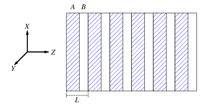
From now on we restrict ourselves to stratified media, which are periodic stacks of dielectric layers. Such systems are also referred to as photonic crystals with one-dimensional periodicity. A major reason for such a choice is that the electrodynamics of stratified media can be done within the framework of a rigorous analytical approach. This is particularly important since the frozen mode regime involves a unique and spectacular behavior, so it would be desirable to be sure that such a behavior is not a numerical artifact. As soon as we assume that the semi-infinite photonic slab in Fig. 2 is a periodic array of plane-parallel uniform layers, we can give a much more detailed and meaningful description of the frozen mode regime.

We start with some general remarks about electromagnetic eigenmodes in periodic layered media. Then we proceed to a semi-qualitative description of the situation taking place at different stationary points of the dispersion relations. A consistent and complete analysis based on the Maxwell equations will be presented in Sections 5 through 12.

3.1 Propagating and evanescent eigenmodes in periodic stacks of anisotropic layers

Let ΨI​(z)\Psi_{I}\left(z\right), ΨR​(z)\Psi_{R}\left(z\right) and ΨT​(z)\Psi_{T}\left(z\right) denote the incident, reflected and transmitted waves, respectively, as shown in Fig. 2. In the frequency domain, each of these waves can be explicitly represented by a column vector

Ψ⁡(z)=[Ex​(z)Ey​(z)Hx​(z)Hy​(z)],\Psi\left(z\right)=\left[\begin{array}[]{c}E_{x}\left(z\right)\\ E_{y}\left(z\right)\\ H_{x}\left(z\right)\\ H_{y}\left(z\right)\end{array}\right], (37)

where Ex​(z),Ey​(z),Hx​(z),Hy​(z)E_{x}\left(z\right),E_{y}\left(z\right),H_{x}\left(z\right),H_{y}\left(z\right)\mathbf{\ }are the transverse components of electromagnetic field. The exact definition of Ψ⁡(z)\Psi\left(z\right) is given in (80) and (81). The incident and reflected beams are plane monochromatic waves propagating in vacuum, while the transmitted electromagnetic field ΨT​(z)\Psi_{T}\left(z\right) inside the periodic layered medium is not a single Bloch eigenmode. At the slab boundary at z=0z=0, the three waves satisfy the standard boundary condition

ΨI​(0)+ΨR​(0)=ΨT​(0),\Psi_{I}\left(0\right)+\Psi_{R}\left(0\right)=\Psi_{T}\left(0\right), (38)

implying continuity of the tangential field components (37). Note that periodic stacks capable of supporting the frozen mode regime must include anisotropic layers with misaligned and/or oblique orientation of the principal axes. As a consequence, the reflected and transmitted waves in Fig. 2 will have an elliptic polarization even if the incident wave is linearly polarized.

In the setting of Fig. 2 where the semi-infinite periodic layered array occupies the half-space z≥0z\geq 0, the transmitted wave ΨT​(z)\Psi_{T}\left(z\right) is a superposition of two Bloch components (Bloch eigenmodes) with different polarizations and different values of the Bloch wave number kk. There are three possibilities.

  1. 1.

    Both Bloch components of the transmitted wave ΨT\Psi_{T} are propagating modes

    ΨT​(z)=Ψp​r​1​(z)+Ψp​r​2​(z),z≥0,\Psi_{T}\left(z\right)=\Psi_{pr1}\left(z\right)+\Psi_{pr2}\left(z\right),\ \;z\geq 0, (39)

    which means that the two respective values of kk are real. For example, at ωb<ω<ωa\omega_{b}<\omega<\omega_{a} in Fig. 1, the transmitted wave ΨT\Psi_{T} is composed of two Bloch eigenmodes with two different real wave numbers k1k_{1} and k2k_{2} and two different group velocities u1>0u_{1}>0 and u2>0u_{2}>0. This constitutes the phenomenon of double refraction.

  2. 2.

    Both Bloch components of ΨT\Psi_{T} are evanescent

    ΨT​(z)=Ψe​v​1​(z)+Ψe​v​2​(z),z≥0,\Psi_{T}\left(z\right)=\Psi_{ev1}\left(z\right)+\Psi_{ev2}\left(z\right),\ \;z\geq 0, (40)

    which implies that the two respective values of kk are complex with I​m⁡k>0\mathop{\mathrm{I}m}k>0. For example, this is the case when the frequency ω\omega falls into the photonic band gap at ω>ωg\omega>\omega_{g} in Fig. 1. The fact that I​m⁡k>0\mathop{\mathrm{I}m}k>0 implies that the wave amplitude decays as the distance zz from the semi-infinite slab surface increases. In the case (40), the incident wave is totally reflected back to space by the semi-infinite slab, as seen in Fig. 3.

  3. 3.

    Of particular interest is the case where one of the Bloch components of the transmitted wave ΨT\Psi_{T} is a propagating mode with u>0u>0, while the other is an evanescent mode with I​m⁡k>0\mathop{\mathrm{I}m}k>0

    ΨT​(z)=Ψp​r​(z)+Ψe​v​(z),z≥0.\Psi_{T}\left(z\right)=\Psi_{pr}\left(z\right)+\Psi_{ev}\left(z\right),\ \;z\geq 0. (41)

    For example, this is the case at the frequency range

    ωa<ω<ωg\omega_{a}<\omega<\omega_{g} (42)

    in Fig. 1. As the distance zz from the slab/vacuum interface increases, the evanescent contribution Ψe​v\Psi_{ev} in (41) decays as exp(−zI​mk)\exp\left(-z\mathop{\mathrm{I}m}k\right), and the resulting transmitted wave ΨT\Psi_{T} turns into a single propagating Bloch mode Ψp​r\Psi_{pr}.

Propagating modes with u<0u<0, as well as evanescent modes with I​m⁡k<0\mathop{\mathrm{I}m}k<0, never contribute to the transmitted wave ΨT\Psi_{T} inside the semi-infinite stack in Fig. 2. This fact is based on the following two assumptions:

  • -

    The transmitted wave ΨT\Psi_{T} and the reflected wave ΨR\Psi_{R} are originated from the plane monochromatic wave ΨI\Psi_{I} incident on the semi-infinite photonic slab from the left, as shown in Fig. 2.

  • -

    The layered array in Fig. 2 occupies the entire half-space and is perfectly periodic at z>0z>0.

If either of the above conditions is violated, the field ΨT\Psi_{T} inside the periodic stack can be a superposition of four Bloch eigenmodes with either sign of the group velocity uu of propagating contributions, or either sign of I​m⁡k\mathop{\mathrm{I}m}k of evanescent contributions. For example, this would be the case if the periodic layered array in Fig. 2 had some kind of structural defects or a finite thickness like that presented in Fig. 6.

The propagating modes with u>0u>0 and evanescent modes with I​m⁡k>0\mathop{\mathrm{I}m}k>0 are referred to as the forward waves. Only forward modes contribute to the transmitted wave ΨT​(z)\Psi_{T}\left(z\right) in the case of a periodic semi-infinite stack. The propagating modes with u<0u<0 and evanescent modes with I​m⁡k<0\mathop{\mathrm{I}m}k<0 are referred to as backward waves. Since the backward Bloch waves are not excited in the setting of Fig. 2, they play no role in further consideration.

In all three cases (39 – 40), the contribution of a particular Bloch eigenmode to the transmitted wave ΨT\Psi_{T} depends on the polarization ΨI\Psi_{I} of the incident wave. One can always choose the incident wave polarization so that only one Bloch component is excited. In such a case, ΨT\Psi_{T} is a single Bloch eigenmode.

Only propagating modes contribute to the normal component STS_{T} of the energy flux inside a periodic semi-infinite slab. Evanescent modes do not participate in energy transfer in such a case. In the important particular case of a single propagating mode (ΨT=Ψp​r\Psi_{T}=\Psi_{pr}), we have from (13) and (14)

ST=W​u=τ​SI,S_{T}=Wu=\tau S_{I}, (43)

where W∼|Ψp​r|2W\sim\left|\Psi_{pr}\right|^{2} is the energy density associated with the transmitted propagating mode.

The assumption that the transmitted wave ΨT​(z)\Psi_{T}\left(z\right) is a superposition of propagating and/or evanescent Bloch eigenmodes may not be valid at stationary points (12) of electromagnetic dispersion function ω⁡(k)\omega\left(k\right), because each stationary point is a degeneracy point of the frequency spectrum. For example, if the frequency ω\omega exactly coincides with stationary inflection point defined by (15), the transmitted wave ΨT​(z)\Psi_{T}\left(z\right) is dominated by a (non-Bloch) Floquet eigenmode linearly growing with zz, which constitutes the frozen mode regime [29, 30]. At all other frequencies, the transmitted wave is a superposition of two forward Bloch modes, each of which can be either propagating or evanescent. A detailed analysis of this and related phenomena is presented further in this paper.

Knowing the eigenmode composition of the transmitted wave ΨT​(z)\Psi_{T}\left(z\right) we can give a semi-qualitative description of what happens when the frequency ω\omega of the incident wave approaches one of the stationary points (12) in Fig. 1. A complete analysis based on the Maxwell equations will be presented later in the paper.

3.2 Photonic band edge

We start with the simplest case of a photonic band edge. Just below the band edge frequency ωg\omega_{g} in Fig. 1, the transmitted field ΨT​(z)\Psi_{T}\left(z\right) is a superposition (41) of one propagating and one evanescent Bloch component. Due to the boundary condition (38) at the slab/vacuum interface, the amplitude of the transmitted wave at z=0z=0 is comparable with that of the incident wave. In the case of a generic polarization of the incident light, the amplitudes of the propagating and evanescent Bloch components at z=0z=0 are also comparable to each other and to the amplitude of the incident light

|Ψp​r(0)|∼|Ψe​v(0)|∼|ΨI|, at ω≤ωg.\left|\Psi_{pr}\left(0\right)\right|\sim\left|\Psi_{ev}\left(0\right)\right|\sim\left|\Psi_{I}\right|,\text{ at }\ \omega\leq\omega_{g}. (44)

As the distance zz from the slab surface increases, the evanescent component Ψe​v​(z)\Psi_{ev}\left(z\right) decays rapidly, while the amplitude of the propagating component remains constant. Eventually, at a certain distance from the slab surface, the transmitted wave ΨT​(z)\Psi_{T}\left(z\right) becomes very close to its propagating Bloch component

ΨT​(z)≈Ψp​r​(z), at ​z≫L,ω≤ωg.\Psi_{T}\left(z\right)\approx\Psi_{pr}\left(z\right),\text{ at }z\gg L,\ \omega\leq\omega_{g}. (45)

The evanescent component Ψe​v\Psi_{ev} of the transmitted wave does not display any singularity in the vicinity of ωg\omega_{g}. By contrast, the propagating mode Ψp​r\Psi_{pr} develops a singularity as ω→ωg−0\omega\rightarrow\omega_{g}-0, which is associated with vanishing group velocity as in (12). At ω>ωg\omega>\omega_{g}, the propagating mode turns into another evanescent mode in (40).

The dispersion relation in the vicinity of the band edge gg in Fig. 1 can be approximated as

ωg−ω≈ωg′′2​(k−kg)2,ω⪅ωg.\omega_{g}-\omega\approx\frac{\omega_{g}^{\prime\prime}}{2}\left(k-k_{g}\right)^{2},\ \ \omega\lessapprox\omega_{g}.

This yields the following frequency dependence of the propagating mode group velocity uu below the photonic band edge

u=∂ω∂k≈ωg′′​(kg−k)≈2​ωg′′​(ωg−ω)1/2,ω⪅ωg.u=\frac{\partial\omega}{\partial k}\approx\omega_{g}^{\prime\prime}\left(k_{g}-k\right)\approx\sqrt{2\omega_{g}^{\prime\prime}}\left(\omega_{g}-\omega\right)^{1/2},\ \ \omega\lessapprox\omega_{g}. (46)

The energy flux (43) associated with the slow propagating mode is

ST≈{W​2​ωg′′​(ωg−ω)1/2, at ​ω⪅ωg0, at ​ω≥ωg.S_{T}\approx\left\{\begin{array}[]{c}W\sqrt{2\omega_{g}^{\prime\prime}}\left(\omega_{g}-\omega\right)^{1/2},\text{ at }\omega\lessapprox\omega_{g}\\ 0,\text{ at }\omega\geq\omega_{g}\end{array}\right.. (47)

where

W∼|Ψp​r|2∼|ΨI|2.W\sim\left|\Psi_{pr}\right|^{2}\sim\left|\Psi_{I}\right|^{2}. (48)

The latter estimation follows from (44) and applies to the case of a generic polarization of the incident wave. The semi-infinite slab transmittance (14) in the vicinity of ωg\omega_{g} is

τ=STSI≈{WSI​2​ωg′′​(ωg−ω)1/2, at ​ω⪅ωg0, at ​ω≥ωg,\tau=\frac{S_{T}}{S_{I}}\approx\left\{\begin{array}[]{c}\frac{W}{S_{I}}\sqrt{2\omega_{g}^{\prime\prime}}\left(\omega_{g}-\omega\right)^{1/2},\text{ at }\omega\lessapprox\omega_{g}\\ 0,\text{ at }\omega\geq\omega_{g}\end{array}\right., (49)

where according to (48)

WSI∼|ΨI|2SI∼c.\frac{W}{S_{I}}\sim\frac{\left|\Psi_{I}\right|^{2}}{S_{I}}\sim c.

The relation (49) is illustrated by the numerical example in Fig. 3.

Equation (49) expresses the well-known fact that in the vicinity of an electromagnetic band edge, the semi-infinite photonic crystal becomes totally reflective, as illustrated in Fig. 3. This implies that as ω→ωg\omega\rightarrow\omega_{g}, only an infinitesimal fraction of the incident light energy is converted into the slow mode.

3.3 Other extreme points of spectral branches

For specificity, let us consider the stationary point aa of the dispersion relation in Fig. 1, which qualitatively is not different from the point bb. At frequencies right below ωa\omega_{a} , the transmitted wave ΨT\Psi_{T} is a superposition (39) of two propagating eigenmodes, one of which is the slow mode and the other is a regular forward propagating mode. The slow mode develops a singularity at ω=ωa\omega=\omega_{a} similar to that of the respective slow mode in the vicinity of the band edge frequency ωg\omega_{g}, while the other propagating mode (the fast mode) remains regular in the vicinity of ωa\omega_{a} and does not produce any anomaly. The two forward modes contribute additively to the energy flux STS_{T}, but the contribution of the fast mode remains regular in the vicinity of ωa\omega_{a}, while the contribution of the slow mode shows the same singular behavior as that described by Eqs. (47) and (49). Fig. 3 provides a graphic illustration of such a behavior.

The important point is that similar to the situation in the vicinity of a photonic band edge, at ω=ωa\omega=\omega_{a} and ω=ωb\omega=\omega_{b} the contribution of the respective slow mode to the transmitted wave ΨT\Psi_{T} vanishes. In other words, in terms of slow mode excitation, the stationary points aa and bb in Fig. 1 are no different from the band edge gg.

3.4 Stationary inflection point: the frozen mode regime

A sharply different situation develops in the vicinity of a stationary inflection point (15) of the dispersion relation (point 00 in Fig. 1). According to (15), the dispersion relation in the vicinity of ω0\omega_{0} can be approximated as follows

ω−ω0≈ω0′′′6​(k−k0)3,\omega-\omega_{0}\approx\frac{\omega_{0}^{\prime\prime\prime}}{6}\left(k-k_{0}\right)^{3}, (50)

where

ω0′′′=(∂3ω∂k3)k=k0.\omega_{0}^{\prime\prime\prime}=\left(\frac{\partial^{3}\omega}{\partial k^{3}}\right)_{k=k_{0}}.

The propagating mode group velocity uu vanishes as ω\omega approaches ω0\omega_{0}

u=∂ω∂k≈12​ω0′′′​(k−k0)2≈62/32​(ω0′′′)1/3​(ω−ω0)2/3.u=\frac{\partial\omega}{\partial k}\approx\frac{1}{2}\omega_{0}^{\prime\prime\prime}\left(k-k_{0}\right)^{2}\approx\frac{6^{2/3}}{2}\left(\omega_{0}^{\prime\prime\prime}\right)^{1/3}\left(\omega-\omega_{0}\right)^{2/3}. (51)

But remarkably, the electromagnetic energy density WW associated with the transmitted frozen mode diverges as ω→ω0\omega\rightarrow\omega_{0}

W≈2​τ​SI62/3(ω0′′′)−1/3(ω−ω0)−2/3,W\approx\frac{2\tau S_{I}}{6^{2/3}}\left(\omega_{0}^{\prime\prime\prime}\right)^{-1/3}\left(\omega-\omega_{0}\right)^{-2/3}, (52)

where SIS_{I} is the fixed energy flux of the incident wave. The slab transmittance τ\tau remains finite even at ω=ω0\omega=\omega_{0}, as illustrated in Fig. 3. As a result, the energy flux (43) associated with the transmitted frozen mode also remains finite and can even be close to unity in the vicinity of ω0\omega_{0}. The latter implies that the incident light is completely converted to the frozen mode with infinitesimal group velocity (51) and diverging energy density (52).

Let us consider the structure of the frozen mode. At ω≈ω0\omega\approx\omega_{0}, the transmitted wave ΨT\Psi_{T} is a superposition (41) of one propagating and one evanescent Bloch component. In contrast to the case of a photonic band edge, in the vicinity of ω0\omega_{0} both Bloch components of ΨT\Psi_{T} develop strong singularity. Specifically, as the frequency ω\omega approaches ω0\omega_{0}, both contributions grow sharply, while remaining nearly equal and opposite in sign at the slab boundary

Ψp​r(0)≈−Ψe​v(0)∝|ω−ω0|−1/3,as ω→ω0.\Psi_{pr}\left(0\right)\approx-\Psi_{ev}\left(0\right)\propto\left|\omega-\omega_{0}\right|^{-1/3},\ \ \text{as }\omega\rightarrow\omega_{0}. (53)

Due to the destructive interference (53), the resulting field

ΨT​(0)=Ψp​r​(0)+Ψe​v​(0)\Psi_{T}\left(0\right)=\Psi_{pr}\left(0\right)+\Psi_{ev}\left(0\right)

at the slab boundary is small enough to satisfy the boundary condition (38), as illustrated in Fig. 8. As the distance zz from the slab boundary increases, the evanescent component Ψe​v\Psi_{ev} decays exponentially

Ψe​v(z)≈Ψe​v(0)exp(−zI​mk)\Psi_{ev}\left(z\right)\approx\Psi_{ev}\left(0\right)\exp\left(-z\mathop{\mathrm{I}m}k\right)

while the amplitude of the propagating component Ψp​r\Psi_{pr} remains constant and very large. As a consequence, the amplitude of the resulting transmitted wave ΨT​(z)\Psi_{T}\left(z\right) sharply increases with the distance zz from the slab boundary and, eventually, reaches its large saturation value corresponding to the propagating component Ψp​r\Psi_{pr}, as illustrated in Fig. 9.

Refer to caption
Figure 8: Destructive interference of the propagating and evanescent contributions to the resulting field ΨT\Psi_{T} at the slab/vacuum interface under the frozen mode regime: a) resulting field amplitude |ΨT​(0)|2\left|\Psi_{T}\left(0\right)\right|^{2}, b) amplitude |Ψp​r​(0)|2\left|\Psi_{pr}\left(0\right)\right|^{2} of the propagating component, c) amplitude |Ψe​v​(0)|2\left|\Psi_{ev}\left(0\right)\right|^{2} of the evanescent component.
Refer to caption
Figure 9: The transmitted electromagnetic field (41) and its propagating and evanescent components inside semi-infinite slab in close proximity of the frozen mode regime: (a) the amplitude |ΨT​(z)|2\left|\Psi_{T}\left(z\right)\right|^{2} of the resulting field, (b) the amplitude |Ψp​r​(z)|2\left|\Psi_{pr}\left(z\right)\right|^{2} of the propagating contribution, (c) the amplitude |Ψe​v​(z)|2\left|\Psi_{ev}\left(z\right)\right|^{2} of the evanescent contribution. Due to destructive interference of the propagating and evanescent components, the resulting field amplitude at z=0z=0 is small enough to satisfy the boundary conditions (38). The amplitude |ΨI|2\left|\Psi_{I}\right|^{2} of the incident wave is unity. The distance zz from the slab boundary is expressed in units of LL.

If the frequency ω\omega of incident light is exactly equal to the frozen mode frequency ω0\omega_{0}, the transmitted wave ΨT​(z)\Psi_{T}\left(z\right) does not reduce to the sum (41) of propagating and evanescent contributions [29, 30]. Instead, it corresponds to a non-Bloch Floquet eigenmode diverging linearly with zz

ΨT​(z)−ΨT​(0)∝z​τ​SIω0′′′​Ψ0,at​ω=ω0.\Psi_{T}\left(z\right)-\Psi_{T}\left(0\right)\propto z\sqrt{\frac{\tau S_{I}}{\omega_{0}^{\prime\prime\prime}}}\Psi_{0},\;\ \text{at}\;\omega=\omega_{0}.

Evidently, the frozen mode regime associated with stationary inflection point (15) provides an ideal and unique situation in terms of slow mode excitation. Indeed, in this case virtually all the incident light energy can be converted into the slow mode with greatly enhanced amplitude.

A consistent mathematical analysis of the frozen mode regime is rather sophisticated and will take a great deal of our attention further in this paper. Specifically, the fundamental fact that at ω=ω0\omega=\omega_{0}, the energy flux of the frozen mode remains finite in spite of vanishing group velocity, is rigorously proven in Section 9 (see Eqs. (561) through (589) and related explanations).

3.5 Degenerate band edge

While the situation with the regular band edge appears quite obvious and not particularly interesting from the perspective of slow light, the so-called degenerate band edge proves to be quite different [34]. An example of an electromagnetic dispersion relation with degenerate band edge is shown in Fig. 10.

Refer to caption
Figure 10: Dispersion relations ω⁡(k)\omega\left(k\right) of three periodic stacks with slightly different layer thicknesses. The plot in the middle displays a degenerate band edge (54).

In the vicinity of the degenerate band edge dd, the dispersion relation can be approximated as

ωd−ω≈ωd′′′′24​(k−kd)4,where ​ωd′′′′=(∂4ω∂k4)k=kd.\omega_{d}-\omega\approx\frac{\omega_{d}^{\prime\prime\prime\prime}}{24}\left(k-k_{d}\right)^{4},\ \text{where }\ \omega_{d}^{\prime\prime\prime\prime}=\left(\frac{\partial^{4}\omega}{\partial k^{4}}\right)_{k=k_{d}}. (54)

Similarly to the regular band edge, below the degenerate band edge frequency ωd\omega_{d}, the transmitted field ΨT\Psi_{T} is a superposition (41) of one propagating and one evanescent components, while above ωd\omega_{d}, the transmitted wave is a combination (40) of two evanescent components. The critical difference though is that now both the Bloch components display strong singularity. Specifically, as the frequency ω\omega approaches ωd\omega_{d}, both Bloch contributions grow sharply, while remaining nearly equal and opposite in sign at the slab boundary

Ψp​r(0)≈−Ψe​v(0)∝|ωd−ω|−1/4,as ω→ωd−0.\Psi_{pr}\left(0\right)\approx-\Psi_{ev}\left(0\right)\propto\left|\omega_{d}-\omega\right|^{-1/4},\ \ \text{as }\omega\rightarrow\omega_{d}-0. (55)

The destructive interference (55) ensures that the boundary condition (38) is satisfied, while both Bloch contributions to ΨT​(z)\Psi_{T}\left(z\right) diverge. As the distance zz from the slab boundary increases, the evanescent component Ψe​v​(z)\Psi_{ev}\left(z\right) dies out, while the propagating component Ψp​r​(z)\Psi_{pr}\left(z\right) remains huge. Eventually, at z≫Lz\gg L, the resulting transmitted wave ΨT​(z)\Psi_{T}\left(z\right) coincides with the propagating Bloch eigenmode Ψp​r​(z)\Psi_{pr}\left(z\right). If the frequency ω\omega of incident light is exactly equal to ωd\omega_{d}, the transmitted wave ΨT​(z)\Psi_{T}\left(z\right) does not reduce to the sum (41) of propagating and evanescent contributions. Instead, it corresponds to a non-Bloch Floquet eigenmode diverging linearly with zz

ΨT​(z)−ΨT​(0)∝z​Ψd,at​ω=ωd.\Psi_{T}\left(z\right)-\Psi_{T}\left(0\right)\propto z\Psi_{d},\;\ \text{at}\;\omega=\omega_{d}.

The above behavior appears to be very similar to that of the frozen mode regime described in the previous subsection. In both cases, Figs. 8 and 9 provide a good graphical illustration of the electromagnetic field distribution inside the slab in the vicinity of the relevant stationary point. Yet, there is a crucial difference between the two cases. In spite of its huge diverging amplitude (55), the transmitted wave ΨT\Psi_{T} does not provide any energy flux in the immediate proximity of a degenerate band edge. Indeed, according to (55), as ω\omega approaches ωd\omega_{d}, the energy density WW of the transmitted wave diverges as

W∝|Ψp​r|2∝|ωd−ω|−1/2, at ω⪅ωd.W\propto\left|\Psi_{pr}\right|^{2}\propto\left|\omega_{d}-\omega\right|^{-1/2},\text{ }\ \ \text{at }\omega\lessapprox\omega_{d}.

But, from Eq. (54) one can derive that the respective slow mode group velocity vanishes even faster

u≈ωd′′′′6(k−kd)3≈243/46(ωd′′′′)1/4|ωd−ω|3/4, at ω⪅ωdu\approx\frac{\omega_{d}^{\prime\prime\prime\prime}}{6}\left(k-k_{d}\right)^{3}\approx\frac{24^{3/4}}{6}\left(\omega_{d}^{\prime\prime\prime\prime}\right)^{1/4}\left|\omega_{d}-\omega\right|^{3/4},\text{ }\ \ \text{at }\omega\lessapprox\omega_{d}

As the result, the energy flux of the transmitted wave vanishes, as one approaches the degenerate band edge

ST=W​u∝{(ωd−ω)1/4, at ​ω⪅ωd0, at ​ω≥ωd,S_{T}=Wu\propto\left\{\begin{array}[]{c}\left(\omega_{d}-\omega\right)^{1/4},\text{ at }\omega\lessapprox\omega_{d}\\ 0,\text{ at }\omega\geq\omega_{d}\end{array}\right.,

and so does the slab transmittance τ\tau

 τ∝{(ωd−ω)1/4, at ​ω⪅ωd0, at ​ω≥ωd.\text{ }\tau\propto\left\{\begin{array}[]{c}\left(\omega_{d}-\omega\right)^{1/4},\text{ at }\omega\lessapprox\omega_{d}\\ 0,\text{ at }\omega\geq\omega_{d}\end{array}\right..

By contrast, in the case of the frozen mode regime the slab transmittance remains finite and a significant fraction of the incident light energy goes to the slow mode.

The situation at a degenerate band edge can be viewed as intermediate between the frozen mode regime and the vicinity of a regular band edge[34]. Indeed, on the one hand, the incident wave at ω=ωd\omega=\omega_{d} is totally reflected back to space, as would be the case at a regular band edge. On the other hand, the transmitted field amplitude inside the slab becomes huge as ω→ωd\omega\rightarrow\omega_{d}, which is similar to what occurs in the frozen mode regime. The large amplitude of the transmitted wave at ω≈ωd\omega\approx\omega_{d} can be very attractive for a variety of practical applications, although such a behavior cannot be qualified as a slow light case. Detailed analysis of some peculiar electromagnetic properties associated with degenerate frequency band edge (54) can be found in [33, 34].

4 Physical conditions for the frozen mode regime in layered media

The frozen mode regime is associated with a stationary inflection point (15) of the electromagnetic dispersion relation. Leaving the proof of this statement to the following sections, here we establish the conditions under which the dispersion relation of a periodic layered array can develop the singularity (15). We will see that only special layered structures incorporating anisotropic layers can display this property. In the following sections, based on the Maxwell equations, we will show that indeed the stationary inflection point (15) is uniquely associated with the frozen mode regime.

4.1 Axial dispersion relation: basic definitions

We start with the generalization of the frozen mode concept to the case of oblique light incidence.

Consider a monochromatic plane wave obliquely incident on a periodic semi-infinite stack, as shown in Fig. 2. Let ΨI\Psi_{I}, ΨR\Psi_{R} and ΨT\Psi_{T} denote the incident, reflected and transmitted waves, respectively. Due to the boundary conditions (38), all three waves ΨI\Psi_{I}, ΨR\Psi_{R} and ΨT\Psi_{T} must be assigned the same pair of tangential components kx,kyk_{x},k_{y} of the respective wave vector [2]

(k→I)x=(k→R)x=(k→T)x,(k→I)y=(k→R)y=(k→T)y,\left(\vec{k}_{I}\right)_{x}=\left(\vec{k}_{R}\right)_{x}=\left(\vec{k}_{T}\right)_{x},\ \ \left(\vec{k}_{I}\right)_{y}=\left(\vec{k}_{R}\right)_{y}=\left(\vec{k}_{T}\right)_{y}, (56)

while their axial (normal) components kzk_{z} can be different. Hereinafter, the normal component of the transmitted Bloch waves propagating inside the periodic layered medium will be referred to as the wave number and denoted by the symbol kk, rather than kzk_{z}, so that inside the periodic stack (at z>0z>0)

k→=(kx,ky,k).\vec{k}=\left(k_{x},k_{y},k\right). (57)

Unlike kxk_{x} and kyk_{y}, the zz component kk of the Bloch wave vector (57) is defined up to a multiple of 2​π/L2\pi/L

k≡k+2​π​N/L,k\equiv k+2\pi N/L, (58)

where LL is the period of the layered structure and NN is an integer. For given kx,kyk_{x},k_{y} and ω\omega, the value kk is found by solving the time-harmonic Maxwell equations (79) in the periodic medium, as will be done in the following sections. The result can be represented as the axial dispersion relation, which gives the relation between ω\omega and kk at fixed kx,kyk_{x},k_{y}

ω=ω⁡(k), at fixed ​kx,ky​.\omega=\omega\left(k\right),\text{\ \ at fixed }k_{x},k_{y}\text{.} (59)

It can be more convenient to define the axial dispersion relation as the relation between ω\omega and kk at fixed direction n→\vec{n} of incident light propagation

ω=ω⁡(k), at fixed ​nx,ny,\omega=\omega\left(k\right),\text{\ \ at fixed }n_{x},n_{y}, (60)

where the unit vector n→\vec{n} can be expressed in terms of the tangential components (56) of the wave vector

nx=kx​c/ω,ny=ky​c/ω,nz=1−(nx2+ny2).n_{x}=k_{x}c/\omega,\ \ n_{y}=k_{y}c/\omega,\ \ n_{z}=\sqrt{1-\left(n_{x}^{2}+n_{y}^{2}\right)}. (61)

4.1.1 Axial stationary inflection point and the frozen mode regime

Suppose that at k→=k→0\vec{k}=\vec{k}_{0}\;and ω=ω0=ω⁡(k→0)\omega=\omega_{0}=\omega\left(\vec{k}_{0}\right), one of the axial spectral branches (59) develops a stationary inflection point for given (kx,ky)(k_{x},k_{y}), namely

at ω=ω0 and k→=k→0: (∂ω∂k)kx,ky=0,(∂2ω∂k2)kx,ky=0,(∂3ω∂k3)kx,ky≠0,\text{at }\omega=\omega_{0}\text{ \ and \ }\vec{k}=\vec{k}_{0}\text{: \ }\left(\frac{\partial\omega}{\partial k}\right)_{k_{x},k_{y}}=0,\;\left(\frac{\partial^{2}\omega}{\partial k^{2}}\right)_{k_{x},k_{y}}=0,\;\left(\frac{\partial^{3}\omega}{\partial k^{3}}\right)_{k_{x},k_{y}}\neq 0, (62)

The value

u≡uz=(∂ω∂k)kx,kyu\equiv u_{z}=\left(\frac{\partial\omega}{\partial k}\right)_{k_{x},k_{y}} (63)

in Eq. (62) is the axial component of the group velocity, which vanishes at k→=k→0\vec{k}=\vec{k}_{0}. Observe that

ux=(∂ω∂kx)k,ky and uy=(∂ω∂ky)k,kx,u_{x}=\left(\frac{\partial\omega}{\partial k_{x}}\right)_{k,k_{y}}\text{ \ and \ }u_{y}=\left(\frac{\partial\omega}{\partial k_{y}}\right)_{k,k_{x}}, (64)

representing the tangential components of the group velocity, may not be zero at k→=k→0\vec{k}=\vec{k}_{0}. The spectral singularity (62) is called the axial stationary inflection point.

One can also use another definition of axial stationary inflection point (62), which is based on the axial dispersion relation (60) rather than (59), namely

at ω=ω0 and n→=n→0: (∂ω∂k)nx,ny=0,(∂2ω∂k2)nx,ny=0,(∂3ω∂k3)nx,ny≠0.\text{at }\omega=\omega_{0}\text{ \ and \ }\vec{n}=\vec{n}_{0}\text{: \ }\left(\frac{\partial\omega}{\partial k}\right)_{n_{x},n_{y}}=0,\;\left(\frac{\partial^{2}\omega}{\partial k^{2}}\right)_{n_{x},n_{y}}=0,\;\left(\frac{\partial^{3}\omega}{\partial k^{3}}\right)_{n_{x},n_{y}}\neq 0. (65)

The partial derivatives in (65) are taken at constant (nx,ny)(n_{x},n_{y}), rather than at constant (kx,ky)(k_{x},k_{y}). Both definitions (62) and (65) are equivalent to one other. In the particular case of normal incidence in which n→|k→|z\vec{n}\parallel\vec{k}\parallel z, the axial stationary inflection point (62) or, equivalently, (65) turns into a regular stationary inflection point (15).

The axial frozen mode regime associated with the singularity (62) is very similar to its particular case, the regular frozen mode regime, related to the regular stationary inflection point (15). Specifically, in the axial frozen mode regime, obliquely incident light can enter the semi-infinite photonic crystal with little reflection, where it is completely converted into a coherent mode with infinitesimal normal component (63) of the group velocity and drastically enhanced amplitude. The energy density of the axial frozen mode displays the same resonance-like behavior (52). The only difference between the axial and the regular frozen mode regime is that in the former case, the tangential component (64) of the group velocity remains finite at ω=ω0\omega=\omega_{0}. The specificity of the axial frozen mode regime as compared to the regular one is discussed in [29]. Further in this paper we will focus exclusively on the common features of these two cases. Either of them will be referred to simply as the frozen mode regime.

4.2 Spectral asymmetry in periodic stacks

The (axial) stationary inflection point is indeed associated with the frozen mode regime. But not every periodic layered media can display such a spectral singularity. It turns out that a necessary condition for the existence of an axial stationary inflection point and, therefore, a necessary condition for the frozen mode regime is the following property of the electromagnetic dispersion relation of the periodic stack

ω⁡(kx,ky,k)≠ω⁡(kx,ky,−k)​ or, equivalently, ​ω​(nx,ny,k)≠ω⁡(nx,ny,−k).\omega\left(k_{x},k_{y},k\right)\neq\omega\left(k_{x},k_{y},-k\right)\text{ \ or, equivalently,\ \ }\omega\left(n_{x},n_{y},k\right)\neq\omega\left(n_{x},n_{y},-k\right). (66)

The property (66) is referred to as axial spectral asymmetry. Further in this paper, we will use the simplified notation (59) for the axial dispersion relation. In this notation, the requirement (66) of axial spectral asymmetry takes the following form

ω⁡(k)≠ω⁡(−k),\omega\left(k\right)\neq\omega\left(-k\right), (67)

where kk is the zz component (58) of the Bloch wave vector k→\vec{k}. A robust frozen mode regime only occurs if the degree of spectral asymmetry (67) is significant. For brevity, hereinafter, the quantity kk will be referred to as the Bloch wave number, although in the case of oblique propagation, kk is just the normal component of the Bloch wave vector k→\vec{k}.

In the particular case of normal wave propagation, in which n→|k→|z\vec{n}\parallel\vec{k}\parallel z, the requirement (66) of axial spectral asymmetry reduces to

ω⁡(k→)≠ω⁡(−k→)​, ​k→|z.\omega\left(\vec{k}\right)\neq\omega\left(-\vec{k}\right)\text{, }\vec{k}\parallel z. (68)

This kind of asymmetric dispersion relation can occur only in periodic structures with some of the constitutive components being magnetic and displaying nonreciprocal Faraday rotation [40, 29]. Significant spectral asymmetry requires strong Faraday rotation. The simplest periodic array supporting the spectral asymmetry (68) is shown in Fig. 11.
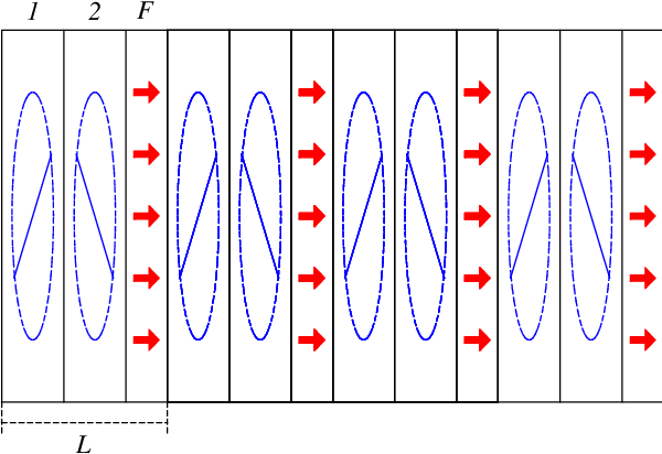
Refer to caption
Figure 11: The simplest periodic stack supporting asymmetric dispersion relation (68). A unit cell LL of this stack comprises three layers: two anisotropic layers 1 and 2 with misaligned in-plane anisotropy (the AA - layers), and one magnetic layer FF with magnetization shown by the arrows.

At microwave frequencies, there exist a number of magnetic materials displaying low losses and strong Faraday rotation. But, at infrared and optical frequencies, the magnetic materials with sufficiently strong Faraday rotation are usually too lossy for our purposes. Therefore, if we are interested in optical frequencies, we have to rely on non-magnetic stacks, in which the regular spectral asymmetry (68) is impossible. By contrast, the axial spectral asymmetry (66) or (67) does not require magnetic layers and can occur even in perfectly reciprocal non-magnetic stacks.

The physical conditions under which the electromagnetic dispersion relation of a non-magnetic layered structure can develop the (axial) spectral asymmetry (67) and, thereby, support the (axial) frozen mode regime can be grouped in two categories. The first one comprises several symmetry restrictions. The second category includes some basic qualitative recommendations which would ensure the robustness of the frozen mode regime, provided that the symmetry conditions for the regime are met. In what follows we briefly describe those conditions and then show how they apply to periodic stacks incorporating some real dielectric materials.

There are two fundamental necessary conditions for the frozen mode regime in a non-magnetic (reciprocal) periodic layered structure. The first one is that the Bloch dispersion function ω⁡(k→)\omega\left(\vec{k}\right) in the periodic layered medium must display the axial spectral asymmetry (67). This condition is necessary for the existence of the axial stationary inflection point (62) in the electromagnetic dispersion relation of an arbitrary periodic layered medium. The second necessary condition is that for the given direction k→\vec{k} of wave propagation, the Bloch eigenmodes Ψk→\Psi_{\vec{k}} with different polarizations must have the same symmetry. In the case of oblique propagation in periodic layered media, the latter condition implies that for the given k→\vec{k}, the Bloch eigenmodes are neither TE nor TM:

Ψk→​ is neither TE nor TM.\Psi_{\vec{k}}\text{ \ is neither TE nor TM.} (69)

The condition (67) imposes certain restrictions on (i) the point symmetry group GG of the periodic layered array and (ii) on the direction k→\vec{k} of the transmitted wave propagation inside the layered medium, while the condition (69) may impose an additional restriction on the direction of k→\vec{k}.

The restriction on the symmetry of the periodic stack stemming from the requirement (67) of the axial spectral asymmetry is

mz∉G​ and ​2z∉G.m_{z}\notin G\text{ \ and \ }2_{z}\notin G. (70)

where mzm_{z} is the mirror plane parallel to the layers, 2z2_{z} is the 2-fold rotation about the zz axis. An immediate consequence of the criterion (70) is that at least one of the alternating layers of the periodic stack must be an anisotropic dielectric with

εx​z≠0​ and/or ​εy​z≠0\varepsilon_{xz}\neq 0\text{ \ \ and/or \ \ }\varepsilon_{yz}\neq 0 (71)

where the zz direction is normal to the layers. Otherwise, the operation 2z2_{z} will be present in the symmetry group GG of the periodic stack.

Refer to caption
Figure 12: Periodic layered structure with two layers AA and BB in a unit cell LL. The AA layers (hatched) are anisotropic with one of the principle axes of the dielectric permittivity tensor ε^\hat{\varepsilon} making an oblique angle with the normal zz to the layers (εx​z≠0\varepsilon_{xz}\neq 0). The BB layers can be isotropic. The x−zx-z plane coincides with the mirror plane mym_{y} of the stack.

The simplest and the most practical example of a non-magnetic periodic stack satisfying the criterion (70) is shown in Fig. 12. It is made up of anisotropic AA layers alternating with isotropic BB layers. The respective dielectric permittivity tensors are

ε^A=[εx​x0εx​z0εy​y0εx​z0εz​z],ε^B=[εB000εB000εB].\hat{\varepsilon}_{A}=\left[\begin{array}[]{ccc}\varepsilon_{xx}&0&\varepsilon_{xz}\\ 0&\varepsilon_{yy}&0\\ \varepsilon_{xz}&0&\varepsilon_{zz}\end{array}\right],\;\hat{\varepsilon}_{B}=\left[\begin{array}[]{ccc}\varepsilon_{B}&0&0\\ 0&\varepsilon_{B}&0\\ 0&0&\varepsilon_{B}\end{array}\right]. (72)

For simplicity, we assume

μ^A=μ^B=I^.\hat{\mu}_{A}=\hat{\mu}_{B}=\hat{I}. (73)

The stack in Fig. 12 has the monoclinic symmetry

2y/my2_{y}/m_{y} (74)

with the mirror plane mym_{y} normal to the yy - axis. Such a symmetry is compatible with the necessary condition (70) for the axial spectral asymmetry (67). Therefore, the periodic array in Fig. 12 can support the frozen mode regime, provided that incident beam lies neither in the x−zx-z, nor in y−xy-x plane [29]

nx≠0​ and ​ny≠0.n_{x}\neq 0\text{ and }n_{y}\neq 0.

If all the above necessary conditions are met, then the (axial) frozen mode regime is, at least, not forbidden by symmetry. More details on the symmetry aspects of the frozen mode regime can be found in [30], Section II and [29], Sections I and II.

In practice, as soon as the symmetry conditions are met, one can almost certainly achieve the (axial) frozen mode regime at any desirable frequency ω\omega within a certain frequency range. The frequency range is determined by the layer thicknesses and the dielectric materials used, while a specific value of ω\omega within the range can be selected by the direction n→\vec{n} of the light incidence. The problem is that unless the physical parameters of the stack layers lie within a certain range, the effects associated with the frozen mode regime can be insignificant or even practically undetectable. The basic guiding principle in choosing appropriate layer materials are discussed in Ref. [30, 33].

The biggest challenge at optical frequencies lies in the fact that most of the commercially available optical anisotropic crystals have weak anisotropy. According to [30], this would push the axial stationary inflection point (62) very close to the photonic band edge and make the photonic crystal almost 100% reflective. This indeed would be the case if we tried to realize the frozen mode regime at the lowest frequency band. But, in Ref. [33] it was shown that the above problem can be successfully solved by moving to a higher frequency band. So, a robust axially frozen mode regime with almost complete conversion of the incident light into the frozen mode can be achieved with the commercially available anisotropic dielectric materials such as N​b​L​i​O3NbLiO_{3}, Y​V​O4YVO_{4}, etc.

5 Electrodynamics of lossless stratified media

This section starts with a description of some basic electrodynamic properties of stratified media composed of lossless anisotropic layers. Then we turn to the important particular case of unbounded periodic layered arrays (periodic stacks), where the electromagnetic eigenmodes are Bloch waves. Then we consider the problem of electromagnetic energy flux in lossless stratified media. Finally, we outline the electromagnetic scattering problem for a semi-infinite photonic slab. The material presented in this section is sufficient for a numerical analysis of slow light phenomena in periodic layered media. This approach was used in [29, 30, 33] to analyze the frozen mode regime in magnetic and non-magnetic periodic stacks. Yet, to develop a consistent analytical picture of the frozen mode regime we shall need a more sophisticated mathematical framework based on a perturbation theory for non-diagonalizable degenerate matrices. This problem will be addressed in the following sections.

5.1 Reduced time-harmonic Maxwell equations

Our treatment is based on the time-harmonic Maxwell equations in heterogeneous nonconducting media

∇×𝐄→​(r→)=i​ωc​𝐁​(r→),∇×𝐇→​(r→)=−i​ωc​𝐃​(r→).\nabla\times\mathbf{\vec{E}}\left(\vec{r}\right)=i\frac{\omega}{c}\mathbf{B}\left(\vec{r}\right),\;\nabla\times\mathbf{\vec{H}}\left(\vec{r}\right)=-i\frac{\omega}{c}\mathbf{D}\left(\vec{r}\right). (75)

Electric and magnetic fields and inductions in Eq. (75) are related through the linear constitutive equations

𝐃→​(r→)=ε^​(r→)​𝐄→​(r→),𝐁→​(r→)=μ^​(r→)​𝐇→​(r→).\mathbf{\vec{D}}\left(\vec{r}\right)=\hat{\varepsilon}\left(\vec{r}\right)\mathbf{\vec{E}}\left(\vec{r}\right),\ \mathbf{\vec{B}}\left(\vec{r}\right)=\hat{\mu}\left(\vec{r}\right)\mathbf{\vec{H}}\left(\vec{r}\right). (76)

All variables in Eqs. (75) and (76) are frequency dependent. In lossless media, the material tensors ε^​(r→)\hat{\varepsilon}\left(\vec{r}\right) and μ^​(r→)\hat{\mu}\left(\vec{r}\right) are Hermitian

In lossless media: ε^(r→)=ε^†(r→),μ^(r→)=μ^†(r→),\text{In lossless media: \ \ }\hat{\varepsilon}\left(\vec{r}\right)=\hat{\varepsilon}^{\dagger}\left(\vec{r}\right),~\hat{\mu}\left(\vec{r}\right)=\hat{\mu}^{\dagger}\left(\vec{r}\right), (77)

where the dagger †\dagger denotes the Hermitian conjugate. In lossless non-magnetic media, both tensors ε^\hat{\varepsilon} and μ^\hat{\mu} are also real and symmetric

In lossless non-magnetic media: ε^(r→)=ε^∗(r→)=ε^T(r→),μ^(r→)=μ^∗(r→)=μ^T(r→),\text{In lossless non-magnetic media: \ \ }\hat{\varepsilon}\left(\vec{r}\right)=\hat{\varepsilon}^{\ast}\left(\vec{r}\right)=\hat{\varepsilon}^{T}\left(\vec{r}\right),~\hat{\mu}\left(\vec{r}\right)=\hat{\mu}^{\ast}\left(\vec{r}\right)=\hat{\mu}^{T}\left(\vec{r}\right), (78)

where the asterisk denotes the complex conjugate and the superscript TT denotes matrix transposition. In magnetically polarized lossless media, the Hermitian material tensors (77) may have a skew-symmetric imaginary part which is responsible for the non-reciprocal effect of Faraday rotation [2].

In a stratified medium, the second rank tensors ε^​(r→)\hat{\varepsilon}\left(\vec{r}\right) and μ^​(r→)\hat{\mu}\left(\vec{r}\right) depend on a single Cartesian coordinate zz, and the Maxwell equations (75) can be recast as

∇×𝐄→​(r→)=i​ωc​μ^​(z)​𝐇→​(r→),∇×𝐇→​(r→)=−i​ωc​ε^​(z)​𝐄→​(r→).\nabla\times\mathbf{\vec{E}}\left(\vec{r}\right)=i\frac{\omega}{c}\hat{\mu}\left(z\right)\mathbf{\vec{H}}\left(\vec{r}\right),\;\nabla\times\mathbf{\vec{H}}\left(\vec{r}\right)=-i\frac{\omega}{c}\hat{\varepsilon}\left(z\right)\mathbf{\vec{E}}\left(\vec{r}\right). (79)

Solutions for Eq. (79) can be sought in the following form

𝐄→​(r→)=ei⁡(kx​x+ky​y)​E→​(z),𝐇→​(r→)=ei⁡(kx​x+ky​y)​H→​(z),\mathbf{\vec{E}}\left(\vec{r}\right)=e^{i\left(k_{x}x+k_{y}y\right)}\vec{E}\left(z\right),\ \mathbf{\vec{H}}\left(\vec{r}\right)=e^{i\left(k_{x}x+k_{y}y\right)}\vec{H}\left(z\right), (80)

which can be interpreted as the “tangential” Bloch representation. The substitution (80) allows separation of the tangential components of the fields into a closed system of four linear ordinary differential equations

∂zΨ⁡(z)=i​ωc​M​(z)​Ψ​(z),Ψ⁡(z)=[Ex​(z)Ey​(z)Hx​(z)Hy​(z)],\partial_{z}\Psi\left(z\right)=i\frac{\omega}{c}M\left(z\right)\Psi\left(z\right),\;\Psi\left(z\right)=\left[\begin{array}[]{c}E_{x}\left(z\right)\\ E_{y}\left(z\right)\\ H_{x}\left(z\right)\\ H_{y}\left(z\right)\end{array}\right], (81)

where the 4×44\times 4 matrix M⁡(z)M\left(z\right) is referred to as the (reduced) Maxwell operator. The normal field components EzE_{z} and HzH_{z} do not enter the reduced Maxwell equations (81) and can be expressed in terms of the tangential field components from Eq. (81) as

Ez=(−nx​Hy+ny​Hx−εx​z∗​Ex−εy​z∗​Ey)​εz​z−1,Hz=(nx​Ey−ny​Ex−μx​z∗​Hx−μy​z∗​Hy)​μz​z−1,\begin{array}[]{c}E_{z}=\left(-n_{x}H_{y}+n_{y}H_{x}-\varepsilon_{xz}^{\ast}E_{x}-\varepsilon_{yz}^{\ast}E_{y}\right)\varepsilon_{zz}^{-1},\\ H_{z}=\left(n_{x}E_{y}-n_{y}E_{x}-\mu_{xz}^{\ast}H_{x}-\mu_{yz}^{\ast}H_{y}\right)\mu_{zz}^{-1},\end{array} (82)

where nx=c​kx/ωn_{x}=ck_{x}/\omega, ny=c​ky/ωn_{y}=ck_{y}/\omega.

The explicit expression for the Maxwell operator M⁡(z)M\left(z\right) in Eq. (81) is

M⁡(z)=[M11M12M21M22]M\left(z\right)=\left[\begin{array}[]{cc}M_{11}&M_{12}\\ M_{21}&M_{22}\end{array}\right] (83)

where

M11\displaystyle M_{11} =[−εx​z∗εz​z​nx−μy​zμz​z​ny(−εy​z∗εz​z+μy​zμz​z)​nx−(εx​z∗εz​z−μx​zμz​z)​ny−εy​z∗εz​z​ny−μx​zμz​z​nx],\displaystyle=\left[\begin{array}[]{cc}-\frac{\varepsilon_{xz}^{\ast}}{\varepsilon_{zz}}n_{x}-\frac{\mu_{yz}}{\mu_{zz}}n_{y}&\left(-\frac{\varepsilon_{yz}^{\ast}}{\varepsilon_{zz}}+\frac{\mu_{yz}}{\mu_{zz}}\right)n_{x}\\ -\left(\frac{\varepsilon_{xz}^{\ast}}{\varepsilon_{zz}}-\frac{\mu_{xz}}{\mu_{zz}}\right)n_{y}&-\frac{\varepsilon_{yz}^{\ast}}{\varepsilon_{zz}}n_{y}-\frac{\mu_{xz}}{\mu_{zz}}n_{x}\end{array}\right],
M22\displaystyle M_{22} =[−εy​zεz​z​ny−μx​z∗μz​z​nx(εy​zεz​z−μy​z∗μz​z)​nx(εx​zεz​z−μx​z∗μz​z)​ny−εx​zεz​z​nx−μy​z∗μz​z​ny],\displaystyle=\left[\begin{array}[]{cc}-\frac{\varepsilon_{yz}}{\varepsilon_{zz}}n_{y}-\frac{\mu_{xz}^{\ast}}{\mu_{zz}}n_{x}&\left(\frac{\varepsilon_{yz}}{\varepsilon_{zz}}-\frac{\mu_{yz}^{\ast}}{\mu_{zz}}\right)n_{x}\\ \left(\frac{\varepsilon_{xz}}{\varepsilon_{zz}}-\frac{\mu_{xz}^{\ast}}{\mu_{zz}}\right)n_{y}&-\frac{\varepsilon_{xz}}{\varepsilon_{zz}}n_{x}-\frac{\mu_{yz}^{\ast}}{\mu_{zz}}n_{y}\end{array}\right],
M12\displaystyle M_{12} =[μx​y∗−μx​z∗​μy​zμz​z+nx​nyεz​zμy​y−μy​z​μy​z∗μz​z−nx2εz​z−μx​x+μx​z​μx​z∗μz​z+ny2εz​z−μx​y+μx​z​μy​z∗μz​z−nx​nyεz​z],\displaystyle=\left[\begin{array}[]{cc}\mu_{xy}^{\ast}-\frac{\mu_{xz}^{\ast}\mu_{yz}}{\mu_{zz}}+\frac{n_{x}n_{y}}{\varepsilon_{zz}}&\mu_{yy}-\frac{\mu_{yz}\mu_{yz}^{\ast}}{\mu_{zz}}-\frac{n_{x}^{2}}{\varepsilon_{zz}}\\ -\mu_{xx}+\frac{\mu_{xz}\mu_{xz}^{\ast}}{\mu_{zz}}+\frac{n_{y}^{2}}{\varepsilon_{zz}}&-\mu_{xy}+\frac{\mu_{xz}\mu_{yz}^{\ast}}{\mu_{zz}}-\frac{n_{x}n_{y}}{\varepsilon_{zz}}\end{array}\right],
M21\displaystyle M_{21} =[−εx​y∗+εx​z∗​εy​zεz​z−nx​nyμz​z−εy​y+εy​z​εy​z∗εz​z+nx2μz​zεx​x−εx​z​εx​z∗εz​z−ny2μz​zεx​y−εx​z​εy​z∗εz​z+nx​nyμz​z].\displaystyle=\left[\begin{array}[]{cc}-\varepsilon_{xy}^{\ast}+\frac{\varepsilon_{xz}^{\ast}\varepsilon_{yz}}{\varepsilon_{zz}}-\frac{n_{x}n_{y}}{\mu_{zz}}&-\varepsilon_{yy}+\frac{\varepsilon_{yz}\varepsilon_{yz}^{\ast}}{\varepsilon_{zz}}+\frac{n_{x}^{2}}{\mu_{zz}}\\ \varepsilon_{xx}-\frac{\varepsilon_{xz}\varepsilon_{xz}^{\ast}}{\varepsilon_{zz}}-\frac{n_{y}^{2}}{\mu_{zz}}&\varepsilon_{xy}-\frac{\varepsilon_{xz}\varepsilon_{yz}^{\ast}}{\varepsilon_{zz}}+\frac{n_{x}n_{y}}{\mu_{zz}}\end{array}\right].

In the important particular case of kx=ky=0k_{x}=k_{y}=0, the Maxwell operator (83) has a simpler form

M⁡(z)=[0M12M210].M\left(z\right)=\left[\begin{array}[]{cc}0&M_{12}\\ M_{21}&0\end{array}\right]. (84)

Only in this case of k→|z\vec{k}\parallel z, the fields E→​(z)\vec{E}\left(z\right) and H→​(z)\vec{H}\left(z\right) coincide with the actual electric and magnetic fields 𝐄→​(r→)\mathbf{\vec{E}}\left(\vec{r}\right) and 𝐇→​(r→)\mathbf{\vec{H}}\left(\vec{r}\right), as follows from the relation (80).

The (reduced) Maxwell operator M⁡(z)M\left(z\right) is a function of:

  • -

    the local values of material tensors ε^​(z)\hat{\varepsilon}\left(z\right) and μ^​(z)\hat{\mu}\left(z\right),

  • -

    the space coordinate zz, via the material tensors ε^​(z)\hat{\varepsilon}\left(z\right) and μ^​(z)\hat{\mu}\left(z\right),

  • -

    the tangential components kx,kyk_{x},k_{y} of the wave vector,

  • -

    the frequency ω\omega.

Different versions of the reduced Maxwell equation (81) can be found in the extensive literature on electrodynamics of stratified media (see, for example, [41] and references therein).

The 4×44\times 4 matrix M⁡(z)M\left(z\right) in Eq. (83) has the fundamental property of JJ-Hermitivity defined as

M†=J​M​J,M^{\dagger}=JMJ, (85)

where

J=J†=J−1=[000100−100−1001000].J=J^{\dagger}=J^{-1}=\left[\begin{array}[]{cccc}0&0&0&1\\ 0&0&-1&0\\ 0&-1&0&0\\ 1&0&0&0\end{array}\right]. (86)

The property (85) relates to conservation of electromagnetic energy in lossless media, it plays an important role in further consideration.

5.2 The transfer matrix formalism

The Cauchy problem

∂zΨ⁡(z)=i​ωc​M​(z)​Ψ​(z),Ψ⁡(z0)=Ψ0\partial_{z}\Psi\left(z\right)=i\frac{\omega}{c}M\left(z\right)\Psi\left(z\right),\;\Psi\left(z_{0}\right)=\Psi_{0} (87)

for the reduced Maxwell equation (81) has a unique solution

Ψ⁡(z)=T⁡(z,z0)​Ψ​(z0)\Psi\left(z\right)=T\left(z,z_{0}\right)\Psi\left(z_{0}\right) (88)

where the 4×44\times 4 matrix T⁡(z,z0)T\left(z,z_{0}\right) is referred to as the transfer matrix. From the definition (88) it follows that

T⁡(z,z0)=T⁡(z,z′)​T​(z′,z0),T⁡(z,z0)=T−1​(z0,z),T⁡(z,z)=I,T\left(z,z_{0}\right)=T\left(z,z^{\prime}\right)T\left(z^{\prime},z_{0}\right),\;T\left(z,z_{0}\right)=T^{-1}\left(z_{0},z\right),\;T\left(z,z\right)=I, (89)

where II is the identity matrix. The transfer matrix T⁡(z,z0)T\left(z,z_{0}\right) allows determination of the time-harmonic electromagnetic field Ψ⁡(z)\Psi\left(z\right) at an arbitrary point zz of the stratified medium once its value Ψ⁡(z0)\Psi\left(z_{0}\right) at any particular point z0z_{0}.

The matrix T⁡(z,z0)T\left(z,z_{0}\right) itself is uniquely defined by the following Cauchy problem

∂zT⁡(z,z0)=i​ωc​M​(z)​T​(z,z0),T⁡(z,z)=I.\partial_{z}T\left(z,z_{0}\right)=i\frac{\omega}{c}M\left(z\right)T\left(z,z_{0}\right),\;T\left(z,z\right)=I. (90)

The equation (90), together with JJ-Hermitivity (85) of the Maxwell operator M⁡(z)M\left(z\right), implies that the transfer matrix T⁡(z,z0)T\left(z,z_{0}\right) is JJ-unitary

T†=J​T−1​J,T^{\dagger}=JT^{-1}J, (91)

as shown in Ref. [30]. The JJ-unitarity (91) of the transfer matrix T=T⁡(z,z0)T=T\left(z,z_{0}\right) imposes the following constraint on its set of four eigenvalues ζi,i=1,2,3,4\zeta_{i},~i=1,2,3,4

{ζ1∗,ζ2∗,ζ3∗,ζ4∗}≡{ζ1−1,ζ2−1,ζ3−1,ζ4−1},\left\{\zeta_{1}^{\ast},\zeta_{2}^{\ast},\zeta_{3}^{\ast},\zeta_{4}^{\ast}\right\}\equiv\left\{\zeta_{1}^{-1},\zeta_{2}^{-1},\zeta_{3}^{-1},\zeta_{4}^{-1}\right\}, (92)

which also implies that

|detT|=1.\left|\det T\right|=1. (93)

5.2.1 The transfer matrix of a stack of uniform layers

The greatest advantage of the transfer matrix approach stems from the fact that the transfer matrix TST_{S} of an arbitrary stack of layers is a sequential product of the transfer matrices TmT_{m} of the constituent layers

TS=∏mTm.T_{S}=\prod_{m}T_{m}. (94)

According to Eq. (90), if each individual layer mm is homogeneous, the corresponding single-layer transfer matrices TmT_{m} can be explicitly expressed in terms of the respective Maxwell operators MmM_{m}

Tm=exp⁡(i​ωc​zm​Mm),T_{m}=\exp\left(i\frac{\omega}{c}z_{m}M_{m}\right), (95)

where zmz_{m} is the thickness of the mm-th layer. The explicit expression for the Maxwell operator MmM_{m} of an arbitrary uniform layer of anisotropic dielectric material is given by Eq. (83). Thus, Eq. (94), together with (95) and (83), give an explicit expression for the transfer matrix TST_{S} of an arbitrary stack of anisotropic dielectric layers. The elements of the JJ-unitary matrix TST_{S} are functions of:

  • -

    the material tensors ε^\hat{\varepsilon} and μ^\hat{\mu} in each layer of the stack,

  • -

    the layer thicknesses dmd_{m},

  • -

    the frequency ω\omega,

  • -

    the tangential components kx=ωc​nx,ky=ωc​nyk_{x}=\frac{\omega}{c}n_{x},\ \ \ k_{y}=\frac{\omega}{c}n_{y} of the wave vector.

In the case of kx=ky=0k_{x}=k_{y}=0, we have instead of Eq. (93)

if ​kx=ky=0​, ​detTS=1,\text{if }k_{x}=k_{y}=0\text{, }\det T_{S}=1, (96)

that can be derived directly from Eqs. (95) and (83).

5.3 Periodic layered arrays. Bloch eigenmodes.

In a periodic layered medium, all material tensors are periodic functions of zz

ε^​(z)=ε^​(z+L),μ^​(z)=μ^​(z+L),\hat{\varepsilon}\left(z\right)=\hat{\varepsilon}\left(z+L\right),~\hat{\mu}\left(z\right)=\hat{\mu}\left(z+L\right),

and so is the Maxwell operator M⁡(z)M(z) in Eq. (81),

M⁡(z+L)=M⁡(z),M\left(z+L\right)=M\left(z\right), (97)

where LL is the length of a unit cell of the periodic stack. A Bloch solution Ψk​(z)\Psi_{k}\left(z\right) of the reduced Maxwell equation (81) with the periodic operator M⁡(z)M(z) should satisfy the following relation

Ψk​(z+L)=ei​k​L​Ψk​(z),\Psi_{k}\left(z+L\right)=e^{ikL}\Psi_{k}\left(z\right), (98)

where kk is the normal component of the Bloch wave vector

k=kz.k=k_{z}. (99)

Unlike kxk_{x} and kyk_{y}, the zz component (99) of the Bloch wave vector is defined up to a multiple of 2​π/L2\pi/L

k≡k+2​π​N/L,k\equiv k+2\pi N/L,

where NN is an integer. Hereinafter, the normal component kzk_{z} of the Bloch wave vector k→\vec{k} will be referred to simply as the wave number and denoted with symbol kk, rather than kzk_{z}.

The definition (88) of the TT-matrix together with Eq. (98) give

Ψk​(z+L)=T⁡(z+L,z)​Ψk​(z)=ei​k​L​Ψk​(z).\Psi_{k}\left(z+L\right)=T\left(z+L,z\right)\Psi_{k}\left(z\right)=e^{ikL}\Psi_{k}\left(z\right). (100)

Introducing the transfer matrix of a primitive cell

TL=T⁡(L,0)T_{L}=T\left(L,0\right) (101)

we have from Eq. (100)

TL​Φk=ei​k​L​Φk, where ​Φk=Ψk​(0).T_{L}\Phi_{k}=e^{ikL}\Phi_{k},\text{ \ \ where }\;\Phi_{k}=\Psi_{k}\left(0\right). (102)

Thus, the eigenvectors of the transfer matrix TLT_{L} of the unit cell are uniquely related to the eigenmodes Ψk​(z)\Psi_{k}\left(z\right) of the reduced Maxwell equation (81) through the relations

Φi=Ψi(0),i=1,2,3,4.\Phi_{i}=\Psi_{i}\left(0\right),\;i=1,2,3,4. (103)

The respective four eigenvalues

ζi=ei​ki​L,i=1,2,3,4\zeta_{i}=e^{ik_{i}L},\;i=1,2,3,4 (104)

of TLT_{L} are the roots of the characteristic equation

F⁡(ζ)=0, where ​F​(ζ)=det(TL−ζ​I^).F\left(\zeta\right)=0,\text{ \ where \ }F\left(\zeta\right)=\det\left(T_{L}-\zeta\hat{I}\right). (105)

For any given ω\omega and (kx,ky)\left(k_{x},k_{y}\right), the characteristic equation (105) defines a set of four values {ζ1,ζ2,ζ3,ζ4}\left\{\zeta_{1},\zeta_{2},\zeta_{3},\zeta_{4}\right\}, or equivalently, {k1,k2,k3,k4}\left\{k_{1},k_{2},k_{3},k_{4}\right\}. Real kk (or, equivalently, |ζ|=1\left|\zeta\right|=1) correspond to propagating Bloch waves (propagating modes), while complex kk (or, equivalently, |ζ|≠1\left|\zeta\right|\neq 1) correspond to evanescent modes. Evanescent modes are relevant near photonic crystal boundaries and other structural irregularities.

The JJ-unitarity (91) of TLT_{L} imposes the restriction (92) on the eigenvalues (104), which can be recast as

{k1,k2,k3,k4}≡{k1∗,k2∗,k3∗,k4∗},\{k_{1},k_{2},k_{3},k_{4}\}\equiv\{k_{1}^{\ast},k_{2}^{\ast},k_{3}^{\ast},k_{4}^{\ast}\}, (106)

for any given ω\omega and kx,kyk_{x},k_{y}. In view of the relations (106) or (92), one can distinguish the following three different situations.

  1. (i)

    All four wave numbers are real

    k1≡k1∗,k2≡k2∗,k3≡k3∗,k4≡k4∗.k_{1}\equiv k_{1}^{\ast},\;k_{2}\equiv k_{2}^{\ast},\;k_{3}\equiv k_{3}^{\ast},\;k_{4}\equiv k_{4}^{\ast}. (107)

    or, equivalently,

    |ζ1|=|ζ2|=|ζ3|=|ζ4|=1.\left|\zeta_{1}\right|=\left|\zeta_{2}\right|=\left|\zeta_{3}\right|=\left|\zeta_{4}\right|=1. (108)

    The respective four Bloch eigenmodes are propagating.

  2. (ii)

    Two real and to complex wave numbers

    k1=k1∗,k2=k2∗,k4=k3∗,where ​k3≠k3∗,k4≠k4∗.k_{1}=k_{1}^{\ast},\;k_{2}=k_{2}^{\ast},\;k_{4}=k_{3}^{\ast},\;\text{where }k_{3}\neq k_{3}^{\ast},\;k_{4}\neq k_{4}^{\ast}. (109)

    or, equivalently,

    |ζ1|=|ζ2|=1,ζ4=1/ζ3∗,where |ζ3|,|ζ4|≠1.\left|\zeta_{1}\right|=\left|\zeta_{2}\right|=1,\ \zeta_{4}=1/\zeta_{3}^{\ast},\;\text{where }\left|\zeta_{3}\right|,\left|\zeta_{4}\right|\neq 1. (110)

    Two of the four Bloch eigenmodes are propagating and the remaining two are evanescent with complex conjugate wave numbers.

  3. (iii)

    All four wave numbers are complex

    k2=k1∗,k4=k3∗,where ​k1≠k1∗,k2≠k2∗,k3≠k3∗,k4≠k4∗.k_{2}=k_{1}^{\ast},\;k_{4}=k_{3}^{\ast},\;\text{where }k_{1}\neq k_{1}^{\ast},\;k_{2}\neq k_{2}^{\ast},\;k_{3}\neq k_{3}^{\ast},\;k_{4}\neq k_{4}^{\ast}. (111)

    or, equivalently,

    ζ2=1/ζ1∗,ζ4=1/ζ3∗,where |ζ1|,|ζ2|,|ζ3|,|ζ4|≠1.\zeta_{2}=1/\zeta_{1}^{\ast},~\zeta_{4}=1/\zeta_{3}^{\ast},\;\text{where }\left|\zeta_{1}\right|,\left|\zeta_{2}\right|,\left|\zeta_{3}\right|,\left|\zeta_{4}\right|\neq 1. (112)

    This situation relates to a frequency gap, where for given ω\omega and kx,kyk_{x},k_{y}, all four Bloch eigenmodes are evanescent.

5.4 Symmetry of the dispersion relation

Below we will see that the dispersion relation is symmetric under k→−kk\rightarrow-k if and only if the transfer matrix TLT_{L} is similar to its inverse. Indeed, assume that

TL=U−1​TL−1​UT_{L}=U^{-1}T_{L}^{-1}U (113)

where UU is a nonsingular 4×44\times 4 matrix. This assumption together with the property (91) of JJ-unitarity, imply also the similarity of TLT_{L} and TL†T_{L}^{\dagger}

TL=V−1​TL†​V,T_{L}=V^{-1}T_{L}^{\dagger}V, (114)

where V=J​UV=JU. Either of the above two relations imposes the following additional restriction on the eigenvalues (104) of TLT_{L} for given ω\omega and kx,kyk_{x},k_{y}

{ζ1,ζ2,ζ3,ζ4}≡{ζ1−1,ζ2−1,ζ3−1,ζ4−1},\{\zeta_{1},\zeta_{2},\zeta_{3},\zeta_{4}\}\equiv\{\zeta_{1}^{-1},\zeta_{2}^{-1},\zeta_{3}^{-1},\zeta_{4}^{-1}\}, (115)

or, equivalently,

{k1,k2,k3,k4}≡{−k1,−k2,−k3,−k4}.\{k_{1},k_{2},k_{3},k_{4}\}\equiv\{-k_{1},-k_{2},-k_{3},-k_{4}\}. (116)

The relation (116) is referred to as axial spectral symmetry. It applies both to propagating and evanescent solutions.

Let us consider the symmetry relation (116) in more detail. Assume that k1=k1∗k_{1}=k_{1}^{\ast} is a real wave number corresponding to a propagating eigenmode. The relation (116) implies that for given ω\omega and kx,kyk_{x},k_{y}, there is another real wave number k2=k2∗k_{2}=k_{2}^{\ast} such that

k2=−k1k_{2}=-k_{1} (117)

In terms of the (axial) dispersion relation ω⁡(k)\omega\left(k\right), the Eq. (117) boils down to a simple definition of axial spectral symmetry

ω⁡(kx,ky,k)=ω⁡(kx,ky,−k),\omega\left(k_{x},k_{y},k\right)=\omega\left(k_{x},k_{y},-k\right),

where k1=kk_{1}=k and k2=−kk_{2}=-k constitute a pair of reciprocal real wave numbers related to given ω\omega and kx,kyk_{x},k_{y}. In the case (107) of four propagating eigenmodes, there will be an additional pair k3k_{3} and k4=−k3k_{4}=-k_{3} of reciprocal wave numbers.

Now assume that while k1k_{1} and k2=−k1k_{2}=-k_{1} are real, the remaining wave numbers k3k_{3} and k4k_{4} from the set (116) are complex, which constitutes the case (109) of two propagating and two evanescent eigenmodes. In such a case, in addition to Eq. (117), the relation (116) together with (106) yields

k4=−k3=k3∗,k_{4}=-k_{3}=k_{3}^{\ast}, (118)

or equivalently

R​ek4=R​ek3=0,π/L;I​mk4=−I​mk3.\mathop{\mathrm{R}e}k_{4}=\mathop{\mathrm{R}e}k_{3}=0,\pi/L;\ \ \ \ \mathop{\mathrm{I}m}k_{4}=-\mathop{\mathrm{I}m}k_{3}. (119)

In Eq. (119) we took into account that k≡k+2​π/Lk\equiv k+2\pi/L.

Consider now the case (111) of a frequency gap, where all four eigenmodes are evanescent. The relations (116) and (106) allow for two different possibilities. The first one is similar to that of Eq. (118)

k2=−k1=k1∗,k4=−k3=k3∗.\begin{array}[]{c}k_{2}=-k_{1}=k_{1}^{\ast},\\ k_{4}=-k_{3}=k_{3}^{\ast}.\end{array} (120)

or, equivalently,

R​ek2=R​ek1=0,π/L;I​mk2=−I​mk1,R​ek4=R​ek3=0,π/L;I​mk4=−I​mk3.\begin{array}[]{c}\mathop{\mathrm{R}e}k_{2}=\mathop{\mathrm{R}e}k_{1}=0,\pi/L;\ \ \mathop{\mathrm{I}m}k_{2}=-\mathop{\mathrm{I}m}k_{1},\\ \mathop{\mathrm{R}e}k_{4}=\mathop{\mathrm{R}e}k_{3}=0,\pi/L;\ \ \mathop{\mathrm{I}m}k_{4}=-\mathop{\mathrm{I}m}k_{3}.\end{array} (121)

In the above situation, the four complex wave numbers split into two reciprocal pairs k1,k2k_{1},k_{2} and k3,k4k_{3},k_{4} of the conjugate values. The other possibility is

k1=−k2∗=k3∗=−k4,k_{1}=-k_{2}^{\ast}=k_{3}^{\ast}=-k_{4}, (122)

or, equivalently,

R​ek1=R​ek3=−R​ek2=−R​ek4,I​mk1=−I​mk3=I​mk2=−I​mk4.\mathop{\mathrm{R}e}k_{1}=\mathop{\mathrm{R}e}k_{3}=-\mathop{\mathrm{R}e}k_{2}=-\mathop{\mathrm{R}e}k_{4},\ \mathop{\mathrm{I}m}k_{1}=-\mathop{\mathrm{I}m}k_{3}=\mathop{\mathrm{I}m}k_{2}=-\mathop{\mathrm{I}m}k_{4}. (123)

5.4.1 Spectral asymmetry

If the sufficient condition (113) for the axial spectral symmetry is not in place, then we can have for given ω\omega and kx,kyk_{x},k_{y}

{k1,k2,k3,k4}≠{−k1,−k2,−k3,−k4},\{k_{1},k_{2},k_{3},k_{4}\}\neq\{-k_{1},-k_{2},-k_{3},-k_{4}\}, (124)

which implies axial spectral asymmetry (67). The relation (106), being a direct consequence of JJ-unitarity (91) of the transfer matrix TLT_{L}, remains valid.

5.5 Electromagnetic energy flux in stratified media

5.5.1 The JJ-scalar product

For future reference, consider the following scalar product involving the JJ-matrix (86)

(Ψ1,J​Ψ2)=E1​x∗​H2​y−E1​y∗​H2​x+H1,y∗​E2​x−H1​x∗​E2​y,\left(\Psi_{1},J\Psi_{2}\right)=E_{1x}^{\ast}H_{2y}-E_{1y}^{\ast}H_{2x}+H_{1,y}^{\ast}E_{2x}-H_{1x}^{\ast}E_{2y},

which will be referred to as the JJ-scalar product. Given the importance of the above quantity, hereinafter, we will use the following special notation for it

[Ψ1,Ψ2]≡(Ψ1,J​Ψ2).\left[\Psi_{1},\Psi_{2}\right]\equiv\left(\Psi_{1},J\Psi_{2}\right). (125)

The JJ-scalar product (125) is invariant under the following transformation involving an arbitrary JJ-unitary matrix TT

[TΨ1,TΨ2]=[Ψ1,Ψ2] for any Ψ1and Ψ2.\left[T\Psi_{1},T\Psi_{2}\right]=\left[\Psi_{1},\Psi_{2}\right]\text{ \ for any }\Psi_{1}\text{and }\Psi_{2}. (126)

The relation (126) can also be viewed as a criterion of JJ-unitarity of a matrix TT. This relation is similar to that involving the regular scalar product (Ψ1,Ψ2)\left(\Psi_{1},\Psi_{2}\right) and a unitary matrix UU

(UΨ1,UΨ2)=(Ψ1,Ψ2) for any Ψ1and Ψ2.\left(U\Psi_{1},U\Psi_{2}\right)=\left(\Psi_{1},\Psi_{2}\right)\text{ \ for any }\Psi_{1}\text{and }\Psi_{2}.

Let Ψi​(z)\Psi_{i}\left(z\right) and Ψj​(z)\Psi_{j}\left(z\right) be two arbitrary solutions of the time-harmonic Maxwell equation (81). The equality (126) together with the definition (88) of the transfer matrix yields

[Ψ​(z)i,Ψj​(z)]=[T⁡(z,0)​Ψ​(0)i,T⁡(z,0)​Ψj​(0)]=[Ψ​(0)i,Ψj​(0)],\left[\Psi\left(z\right)_{i},\Psi_{j}\left(z\right)\right]=\left[T\left(z,0\right)\Psi\left(0\right)_{i},T\left(z,0\right)\Psi_{j}\left(0\right)\right]=\left[\Psi\left(0\right)_{i},\Psi_{j}\left(0\right)\right], (127)

which implies that the JJ-scalar product [Ψ​(z)i,Ψj​(z)]\left[\Psi\left(z\right)_{i},\Psi_{j}\left(z\right)\right] does not depend on the coordinate zz.

Consider now the JJ-scalar product

[Φi,Φj]\left[\Phi_{i},\Phi_{j}\right] (128)

of two eigenvectors Φi\Phi_{i} and Φj\Phi_{j} of the transfer matrix TLT_{L}

TLΦi=ζiΦi,i=1,2,3,4.T_{L}\Phi_{i}=\zeta_{i}\Phi_{i},\;i=1,2,3,4. (129)

The JJ-unitarity (126) of TLT_{L} implies that

[TL​Φi,TL​Φj]=ζi∗​ζj​[Φi,Φj]=[Φi,Φj],\left[T_{L}\Phi_{i},T_{L}\Phi_{j}\right]=\zeta_{i}^{\ast}\zeta_{j}\left[\Phi_{i},\Phi_{j}\right]=\left[\Phi_{i},\Phi_{j}\right], (130)

which, in turn, yields the following important relation

[Φi,Φj]=0, if ​ζi∗​ζj≠1,\left[\Phi_{i},\Phi_{j}\right]=0,\text{ \ if \ }\zeta_{i}^{\ast}\zeta_{j}\neq 1, (131)

or equivalently,

[Φi,Φj]=0, if ​kj≠ki∗.\left[\Phi_{i},\Phi_{j}\right]=0,\text{ \ if \ }k_{j}\neq k_{i}^{\ast}. (132)

In particular

[Φi,Φi]≠0, only if ​ki=ki∗,\left[\Phi_{i},\Phi_{i}\right]\neq 0,\text{ \ only if \ }k_{i}=k_{i}^{\ast}, (133)

which means that Φi\Phi_{i} in (133) should be a propagating Bloch mode.

5.5.2 Energy flux in stratified media

The real-valued energy flux (the Poynting vector) associated with a time-harmonic electromagnetic field is

𝐒⁡(r→)=[R​e⁡𝐄⁡(r→)×R​e⁡𝐇⁡(r→)]=12​R​e⁡[𝐄∗​(r→)×𝐇⁡(r→)].\mathbf{S}\left(\vec{r}\right)=\left[\mathop{\mathrm{R}e}\mathbf{E}\left(\vec{r}\right)\times\mathop{\mathrm{R}e}\mathbf{H}\left(\vec{r}\right)\right]=\frac{1}{2}\mathop{\mathrm{R}e}\left[\mathbf{E}^{\ast}\left(\vec{r}\right)\times\mathbf{H}\left(\vec{r}\right)\right]. (134)

Substitution of the “tangential” Bloch representation (80) for 𝐄⁡(r→)\mathbf{E}\left(\vec{r}\right) and 𝐇⁡(r→)\mathbf{H}\left(\vec{r}\right) in Eq. (134) yields

𝐒⁡(r→)=𝐒⁡(z)=12​R​e⁡[E→∗​(z)×H→​(z)],\mathbf{S}\left(\vec{r}\right)=\mathbf{S}\left(z\right)=\frac{1}{2}\mathop{\mathrm{R}e}\left[\vec{E}^{\ast}\left(z\right)\times\vec{H}\left(z\right)\right], (135)

at fixed ω\omega and kx,kyk_{x},k_{y}. Eq. (135) implies that in a stratified medium, at fixed ω\omega and kx,kyk_{x},k_{y}, all three Cartesian components of the energy flux 𝐒⁡(r→)\mathbf{S}\left(\vec{r}\right) are independent of the tangential coordinates xx and yy. A simple energy conservation argument shows that the normal component SzS_{z} of the energy flux does not depend on the coordinate zz either, while the tangential components SxS_{x} and SyS_{y} may depend on zz. Indeed, in a lossless stratified medium we have, with consideration for Eq. (135)

∇⋅𝐒⁡(r→)=∂zSz​(z)=0,\nabla\cdot\mathbf{S}\left(\vec{r}\right)=\partial_{z}S_{z}\left(z\right)=0,

which yields that at fixed ω\omega and kx,kyk_{x},k_{y}

Sz​(r→)=Sz=const.S_{z}\left(\vec{r}\right)=S_{z}=\text{const}. (136)

By contrast, the tangential components of the steady-state energy flux are dependent on the zz coordinate

Sx​(r→)=Sx​(z),Sy​(r→)=Sy​(z).S_{x}\left(\vec{r}\right)=S_{x}\left(z\right),\;S_{y}\left(\vec{r}\right)=S_{y}\left(z\right). (137)

Hereinafter, the normal component of the energy flux will be referred to simply as the energy flux, unless otherwise specifically stated. It also will be denoted as SS, rather than SzS_{z}.

The explicit expression for the normal component of the energy flux (135) can be recast as

S=12​(Ex∗​Hy−Ey∗​Hx+Ex​Hy∗−Ey​Hx∗)=12​[Ψ,Ψ],S=\frac{1}{2}\left(E_{x}^{\ast}H_{y}-E_{y}^{\ast}H_{x}+E_{x}H_{y}^{\ast}-E_{y}H_{x}^{\ast}\right)=\frac{1}{2}\left[\Psi,\Psi\right], (138)

where the JJ-scalar product [Ψ,Ψ]≡(Ψ,J​Ψ)\left[\Psi,\Psi\right]\equiv\left(\Psi,J\Psi\right) is defined in Eq. (125). The fact that SS in Eq. (138) is independent of zz implies that

S=12​[Ψ⁡(z),Ψ⁡(z)]=12​[Φ,Φ], where ​Φ=Ψ⁡(0).S=\frac{1}{2}\left[\Psi\left(z\right),\Psi\left(z\right)\right]=\frac{1}{2}\left[\Phi,\Phi\right],\text{ \ where }\Phi=\Psi\left(0\right). (139)

Eq. (139) can also be viewed as a direct consequence of JJ-unitarity (91) of the transfer matrix. Indeed, from the definition (88) of the transfer matrix we have

Ψ⁡(z)=T⁡(z,0)​Ψ​(0)=T⁡(z,0)​Φ.\Psi\left(z\right)=T\left(z,0\right)\Psi\left(0\right)=T\left(z,0\right)\Phi. (140)

Substituting (140) into (138) yields

S=12​[Ψ⁡(z),Ψ⁡(z)]=12​[T⁡(z,0)​Φ,T⁡(z,0)​Φ].S=\frac{1}{2}\left[\Psi\left(z\right),\Psi\left(z\right)\right]=\frac{1}{2}\left[T\left(z,0\right)\Phi,T\left(z,0\right)\Phi\right].

Taking into account the property (126) of a JJ-unitary matrix, we again arrive at Eq. (139).

5.5.3 Energy flux in periodic stratified media

The direct relation (139) between the JJ-scalar product [Ψ,Ψ]\left[\Psi,\Psi\right] and the energy flux SS at fixed ω\omega and kx,kyk_{x},k_{y} allows us to make some strong statements regarding electromagnetic energy flux in periodic layered media.

Let us start with the simplest case of a single Bloch eigenmode. Eq. (139) together with (133) shows that only a propagating mode can transfer electromagnetic energy

Si=12​[Φi,Φi]≠0​ only if ​ki=ki∗.S_{i}=\frac{1}{2}\left[\Phi_{i},\Phi_{i}\right]\neq 0\text{ only if }k_{i}=k_{i}^{\ast}. (141)

A single evanescent eigenmode always has zero energy flux

Si=[Φi,Φi]=0, if ​ki≠ki∗.S_{i}=\left[\Phi_{i},\Phi_{i}\right]=0,\text{ \ if \ }k_{i}\neq k_{i}^{\ast}. (142)

Let us turn to the case of a superposition

Φ=∑i=14ai​Φi.\Phi=\mathop{\displaystyle\sum}\limits_{i=1}^{4}a_{i}\Phi_{i}.

of different Bloch eigenmodes with fixed ω\omega and kx,kyk_{x},k_{y}. In such a case, the energy flux is

S=12​[Φ,Φ]=12​∑i,j=14ai∗​aj​[Φi,Φj].S=\frac{1}{2}\left[\Phi,\Phi\right]=\frac{1}{2}\mathop{\displaystyle\sum}\limits_{i,j=1}^{4}a_{i}^{\ast}a_{j}\left[\Phi_{i},\Phi_{j}\right]. (143)

Taking into account Eqs. (132) we can draw the following conclusions:

  1. 1)

    The contribution SiS_{i} of each propagating eigenmode to the total energy flux is independent of the presence or absence of other Bloch eigenmodes with the same ω\omega and kx,kyk_{x},k_{y}

    S=∑i=1Si=12​∑i=1|ai|2​[Φi,Φi],S=\mathop{\displaystyle\sum}\limits_{i=1}S_{i}=\frac{1}{2}\mathop{\displaystyle\sum}\limits_{i=1}\left|a_{i}\right|^{2}\left[\Phi_{i},\Phi_{i}\right], (144)

    where the summation runs over all propagating eigenmodes. The number of propagating modes can be 4, 2, or 0, depending on which of the cases (111), (109), or (111) we are dealing with.

  2. 2)

    The contribution of evanescent Bloch eigenmodes to the energy flux depends on their number.

    1. (a)

      In the case (109) of two evanescent modes Φ3\Phi_{3} and Φ4\Phi_{4} we have

      S=R​e⁡(a3∗​a4​[Φ3,Φ4]), where ​k4=k3∗,S=\mathop{\mathrm{R}e}\left(a_{3}^{\ast}a_{4}\left[\Phi_{3},\Phi_{4}\right]\right),\text{ where }k_{4}=k_{3}^{\ast}, (145)

      which implies that only a pair of evanescent modes with conjugate wave numbers can produce energy flux. The respective contribution (145) is independent of the presence of propagating modes Φ1\Phi_{1} and Φ2\Phi_{2}. In accordance with Eq. (142), a single evanescent mode, either Φ3\Phi_{3} or Φ4\Phi_{4}, does not produce energy flux on its own.

    2. (b)

      In the case (111) of four evanescent modes we have

      S=R​e⁡(a1∗​a2​[Φ1,Φ2])+R​e⁡(a3∗​a4​[Φ3,Φ4]), where ​k2=k1∗,k4=k3∗,S=\mathop{\mathrm{R}e}\left(a_{1}^{\ast}a_{2}\left[\Phi_{1},\Phi_{2}\right]\right)+\mathop{\mathrm{R}e}\left(a_{3}^{\ast}a_{4}\left[\Phi_{3},\Phi_{4}\right]\right),\text{ where }k_{2}=k_{1}^{\ast},k_{4}=k_{3}^{\ast}, (146)

      which implies that either of the two pairs of evanescent modes with conjugate wave numbers contribute to the energy flux independently of each other.

5.6 Scattering problem for a periodic semi-infinite stack

In this final subsection we outline the standard procedure we use for solving the scattering problem of a plane monochromatic wave incident on the surface of a periodic semi-infinite stack.

In vacuum (to the left of the semi-infinite slab) the electromagnetic field ΨV​(z)\Psi_{V}\left(z\right) is a superposition of the incident and reflected waves

ΨV(z)=ΨI(z)+ΨR(z), z≤0,\Psi_{V}\left(z\right)=\Psi_{I}\left(z\right)+\Psi_{R}\left(z\right),\text{ }z\leq 0, (147)

where the indices II and RR relate to the incident and reflected beams, respectively. At the slab boundary we have

ΨV​(0)=ΨI​(0)+ΨR​(0).\Psi_{V}\left(0\right)=\Psi_{I}\left(0\right)+\Psi_{R}\left(0\right). (148)

The transmitted wave ΨT​(z)\Psi_{T}\left(z\right) inside the periodic semi-infinite slab is a superposition of two forward Bloch eigenmodes

ΨT(z)=Ψ1(z)+Ψ2(z), z≥0.\Psi_{T}\left(z\right)=\Psi_{1}\left(z\right)+\Psi_{2}\left(z\right),\text{ }z\geq 0. (149)

The eigenmodes Ψ1​(z)\Psi_{1}\left(z\right)\ and Ψ2​(z)\Psi_{2}\left(z\right) can be both propagating (with u>0u>0), one propagating and one evanescent (with u>0u>0 and I​m⁡k>0,\mathop{\mathrm{I}m}k>0, respectively), or both evanescent (with I​m⁡k>0\mathop{\mathrm{I}m}k>0), depending on which of the three cases (39), (41), or (40) we are dealing with.

Assume now that for a given frequency ω\omega, the Bloch eigenmodes are found, which can be readily done in the case of a periodic layered array. Using the standard electromagnetic boundary conditions

ΨT​(0)=ΨI​(0)+ΨR​(0),\Psi_{T}\left(0\right)=\Psi_{I}\left(0\right)+\Psi_{R}\left(0\right), (150)

one can express the reflected wave ΨR\Psi_{R} and the eigenmode composition of the transmitted wave ΨT\Psi_{T}, in terms of the amplitude and polarization of the incident wave ΨI\Psi_{I}. This automatically gives the electromagnetic field distribution ΨT​(z)\Psi_{T}\left(z\right) inside the slab, as a function of the incident wave frequency, polarization, and direction of incidence.

The transmittance and reflectance coefficients of a lossless semi-infinite slab are defined by the following expressions

τ=1−ρ=(S→T)z(S→I)z,ρ=−(S→R)z(S→I)z.\tau=1-\rho=\frac{\left(\vec{S}_{T}\right)_{z}}{\left(\vec{S}_{I}\right)_{z}},\;\;\rho=-\frac{\left(\vec{S}_{R}\right)_{z}}{\left(\vec{S}_{I}\right)_{z}}. (151)

where (S→I)z\left(\vec{S}_{I}\right)_{z} , (S→R)z\left(\vec{S}_{R}\right)_{z} and (S→T)z\left(\vec{S}_{T}\right)_{z}are the normal components of the energy flux of the incident, reflected, and transmitted waves, respectively. Knowing the value of the transmitted wave ΨT\Psi_{T} or reflected wave ΨR\Psi_{R} at the slab boundary, one can immediately find the respective energy flux and, thereby, the transmittance/reflectance coefficients (151).

The above-outlined standard procedure was used in all our numerical simulations. It applies both to the case of normal and oblique incidence. In the latter case, the explicit expressions for the column vectors ΨI\Psi_{I} and ΨR\Psi_{R} in (147-150) are

ΨI=[EI,xEI,yHI,xHI,y],ΨR=[ER,xER,yHR,xHR,y],\Psi_{I}=\left[\begin{array}[]{c}E_{I,x}\\ E_{I,y}\\ H_{I,x}\\ H_{I,y}\end{array}\right],\ \ \Psi_{R}=\left[\begin{array}[]{c}E_{R,x}\\ E_{R,y}\\ H_{R,x}\\ H_{R,y}\end{array}\right], (152)

where the complex vectors E→I,H→I\vec{E}_{I},\vec{H}_{I} and E→R,H→R\vec{E}_{R},\vec{H}_{R} are related to the actual electromagnetic field components 𝐄I,𝐇I\mathbf{E}_{I},\mathbf{H}_{I} and 𝐄R,𝐇R\mathbf{E}_{R},\mathbf{H}_{R} as

𝐄→I\displaystyle\mathbf{\vec{E}}_{I} =ei​ωc​(nx​x+ny​y)​E→I​(z),𝐇→I=ei​ωc​(nx​x+ny​y)​H→I,\displaystyle=e^{i\frac{\omega}{c}\left(n_{x}x+n_{y}y\right)}\vec{E}_{I}\left(z\right),\ \mathbf{\vec{H}}_{I}=e^{i\frac{\omega}{c}\left(n_{x}x+n_{y}y\right)}\vec{H}_{I}, (153)
𝐄→R\displaystyle\mathbf{\vec{E}}_{R} =ei​ωc​(nx​x+ny​y)​E→R​(z),𝐇→R=ei​ωc​(nx​x+ny​y)​H→R,\displaystyle=e^{i\frac{\omega}{c}\left(n_{x}x+n_{y}y\right)}\vec{E}_{R}\left(z\right),\ \mathbf{\vec{H}}_{R}=e^{i\frac{\omega}{c}\left(n_{x}x+n_{y}y\right)}\vec{H}_{R}, (154)

as prescribed by Eq. (80). Here n→\vec{n} is the unit vector in the direction of light propagation

for incident beam: n→=n→I=(cωkx,cωky,cωkz),\text{for incident beam: \ \ }\vec{n}=\vec{n}_{I}=\left(\frac{c}{\omega}k_{x},\frac{c}{\omega}k_{y},\frac{c}{\omega}k_{z}\right), (155)
for reflected beam: n→=n→R=(cωkx,cωky,−cωkz),\text{for reflected beam: \ \ }\vec{n}=\vec{n}_{R}=\left(\frac{c}{\omega}k_{x},\frac{c}{\omega}k_{y},-\frac{c}{\omega}k_{z}\right), (156)

where

kz=cω​nz=cω​1−(nx2+ny2).k_{z}=\frac{c}{\omega}n_{z}=\frac{c}{\omega}\sqrt{1-\left(n_{x}^{2}+n_{y}^{2}\right)}.

Note that the tangential components of the unit vector n→\vec{n} of the incident wave are the same as those of the reflected wave. The electric and magnetic fields of a plane monochromatic wave in a vacuum are uniquely related to each other

𝐇→=n→×𝐄→.\mathbf{\vec{H}}=\vec{n}\times\mathbf{\vec{E}}.

The same relation holds for the complex vectors E→I,H→I\vec{E}_{I},\vec{H}_{I} and E→R,H→R\vec{E}_{R},\vec{H}_{R} defined in (153) and (154), namely

H→I=n→I×E→I,H→R=n→R×E→R.\vec{H}_{I}=\vec{n}_{I}\times\vec{E}_{I},\ \ \vec{H}_{R}=\vec{n}_{R}\times\vec{E}_{R}. (157)

6 Matrix of reflection coefficients of a semi-infinite periodic stack

This and the following sections are devoted to a rigorous mathematical analysis of the scattering problem for a plane monochromatic wave incident on a periodic semi-infinite stack. We focus on vicinities of stationary points of the electromagnetic dispersion relation and our goal is to develop an asymptotic analytical description of the frozen mode regime. Not only that would allow to rigorously prove the physical results presented earlier in this paper, it would also provide a better understanding of the very essence of the frozen mode regime. The major part of the following analysis is a perturbation theory of degenerate non-diagonalizable matrices. Specifically, we refer to the transfer matrix TLT_{L}, which develops a nontrivial Jordan block at any stationary point of the dispersion relations. The latter circumstance implies the existence of diverging non-Bloch eigenmodes, which usually do not contribute to the transmitted wave ΨT\Psi_{T} inside the semi-infinite photonic slab and, therefore, do not affect the scattering problem at hand. Yet, there are two important exceptions. The first one is the stationary inflection point (15), where not only the linearly diverging Floquet eigenmode dominates the transmitted wave, but it also produces a finite energy flux inside the periodic medium. Another exception is the degenerate band edge (54), where the respective linearly divergent non-Bloch eigenmode, although dominant, does not contribute to the energy flux and, therefore, does not effectively transform the incident radiation into the slow mode.

The rest of the paper is organized as follows. In this section we re-formulate the scattering problem for a lossless periodic semi-infinite stack, introducing basic notations and definitions. In the following sections we develop a perturbation theory for degenerate non-diagonalizable 4×44\times 4 matrices and apply this theory to the transfer matrix TLT_{L} and, thereby, to the scattering problem. Special attention is given to the comparative analysis of different stationary points of the electromagnetic dispersion relation, such as a photonic band edge, a stationary inflection point, and a degenerate band edge. To simplify the rather cumbersome mathematical expressions of the following sections, we will use the following new notations for the quantities already defined earlier

x1\displaystyle x_{1} →x,x2→y,x3→z,\displaystyle\rightarrow x,\ x_{2}\rightarrow y,x_{3}\rightarrow z,
A\displaystyle A →ωc​J​M,T→TL,\displaystyle\rightarrow\frac{\omega}{c}JM,\;T\rightarrow T_{L},
𝐤\displaystyle\mathbf{k} =(k1,k2,k3)→(c​kx,c​ky,c​kz).\displaystyle=\left(k_{1},k_{2},k_{3}\right)\rightarrow\left(ck_{x},ck_{y},ck_{z}\right).

Observe that the 4×44\times 4 matrix

A=ωc​J​MA=\frac{\omega}{c}JM (158)

is Hermitian, while the related Maxwell operator MM defined in Eqs. (81-86) is JJ-Hermitian.

6.1 Basic definitions

A periodic semi-infinite stack is defined in terms of the related matrix function A⁡(x3)A\left(x_{3}\right) satisfying

A(x3)=C​o​n​s​t,−∞<x3<0;A(x3+L)=A(x3), 0<x3<∞.A\left(x_{3}\right)=\mathop{\mathrm{C}onst},\ -\infty<x_{3}<0;\ A\left(x_{3}+L\right)=A\left(x_{3}\right),\ 0<x_{3}<\infty. (159)

In vacuum, the Hermitian matrix A⁡(x3)A\left(x_{3}\right) defined in (158) and has the form

A⁡(x3)=A(0)=[𝐚(0)𝟎𝟎𝐚(0)],𝐚(0)=1ω​[ω2−k22k1​k2k1​k2ω2−k12],A\left(x_{3}\right)=A^{\left(0\right)}=\left[\begin{array}[]{cc}\mathbf{a}^{\left(0\right)}&\mathbf{0}\\ \mathbf{0}&\mathbf{a}^{\left(0\right)}\end{array}\right],\ \mathbf{a}^{\left(0\right)}=\frac{1}{\omega}\left[\begin{array}[]{cc}\omega^{2}-k_{2}^{2}&k_{1}k_{2}\\ k_{1}k_{2}&\omega^{2}-k_{1}^{2}\end{array}\right], (160)

The above expressions immediately follow from Eqs. (83) and (158). The tangential component 𝐤τ\mathbf{k}_{\tau} of the the wave vector 𝐤\mathbf{k} is related to its normal component k3k_{3} by

k3=ω2−𝐤τ2=ω2−(k12+k22).k_{3}=\sqrt{\omega^{2}-\mathbf{k}_{\tau}^{2}}=\sqrt{\omega^{2}-\left(k_{1}^{2}+k_{2}^{2}\right)}. (161)

Let us introduce

j2=[0−110],J=[0−j2j20]=j2⊗j2,j_{2}=\left[\begin{array}[]{cc}0&-1\\ 1&0\end{array}\right],\ J=\left[\begin{array}[]{cc}0&-j_{2}\\ j_{2}&0\end{array}\right]=j_{2}\otimes j_{2}, (162)

and notice that

J​A(0)=[0−j2​𝐚(0)j2​𝐚(0)0]=[0−110]⊗[j2​𝐚(0)]=j2⊗[j2​𝐚(0)].JA^{\left(0\right)}=\left[\begin{array}[]{cc}0&-j_{2}\mathbf{a}^{\left(0\right)}\\ j_{2}\mathbf{a}^{\left(0\right)}&0\end{array}\right]=\left[\begin{array}[]{cc}0&-1\\ 1&0\end{array}\right]\otimes\left[j_{2}\mathbf{a}^{\left(0\right)}\right]=j_{2}\otimes\left[j_{2}\mathbf{a}^{\left(0\right)}\right]. (163)

Recall the basic properties of the tensor product operation: if AA and BB are square matrices and uu and vv are vectors of related dimensions then

[A⊗B]​(u⊗v)=(A​u)⊗(B​v),(u1⊗v1,u2⊗v2)=(u1,u2)​(v1,v2).\left[A\otimes B\right]\left(u\otimes v\right)=\left(Au\right)\otimes\left(Bv\right),\ \left(u_{1}\otimes v_{1},u_{2}\otimes v_{2}\right)=\left(u_{1},u_{2}\right)\left(v_{1},v_{2}\right). (164)

Suppose now that we know the set of eigenvectors and eigenvalues for two square matrices AA and BB, namely

A​uj=λj​uj,B​vm=μm​vm.Au_{j}=\lambda_{j}u_{j},\ Bv_{m}=\mu_{m}v_{m}. (165)

Then (164) and (165) imply

[A⊗B]​(uj⊗vm)=λj​μm​uj⊗vm.\left[A\otimes B\right]\left(u_{j}\otimes v_{m}\right)=\lambda_{j}\mu_{m}u_{j}\otimes v_{m}. (166)

Using (166) and the tensor product representation (163) for J​A(0)JA^{\left(0\right)} we can find its eigenvectors and eigenvalues as follows. First, we find that

j2​u±\displaystyle j_{2}u_{\pm} =±i​u±,u±=12​[±i1];j2​𝐚(0)​v±=±i​k3​v±,\displaystyle=\pm\mathrm{i}u_{\pm},\ u_{\pm}=\frac{1}{\sqrt{2}}\left[\begin{array}[]{c}\pm\mathrm{i}\\ 1\end{array}\right];\ \ \ j_{2}\mathbf{a}^{\left(0\right)}v_{\pm}=\pm\mathrm{i}k_{3}v_{\pm},
v±\displaystyle v_{\pm} =v±​(ω,𝐤τ)=1γω,𝐤τ​[−k32+k22±i​ω​k3+k1​k21],γω,𝐤τ=2​(k32+k22)​k3​ωω2​k32+k12​k22.\displaystyle=v_{\pm}\left(\omega,\mathbf{k}_{\tau}\right)=\frac{1}{\gamma_{\omega,\mathbf{k}_{\tau}}}\left[\begin{array}[]{c}-\frac{k_{3}^{2}+k_{2}^{2}}{\pm\mathrm{i}\omega k_{3}+k_{1}k_{2}}\\ 1\end{array}\right],\ \ \gamma_{\omega,\mathbf{k}_{\tau}}=\sqrt{\frac{2\left(k_{3}^{2}+k_{2}^{2}\right)k_{3}\omega}{\omega^{2}k_{3}^{2}+k_{1}^{2}k_{2}^{2}}}.

Notice also that

(v+,j2​v−)\displaystyle\left(v_{+},j_{2}v_{-}\right) =(v−,j2​v+)=0,(v±,j2​v±)=±i,\displaystyle=\left(v_{-},j_{2}v_{+}\right)=0,\ \left(v_{\pm},j_{2}v_{\pm}\right)=\pm\mathrm{i}, (171)
(v±,v±)\displaystyle\left(v_{\pm},v_{\pm}\right) =βω,𝐤τ=(k32+k22)2+(ω​k3)2+(k1​k2)22​(k32+k22)​k3​ω,\displaystyle=\beta_{\omega,\mathbf{k}_{\tau}}=\frac{\left(k_{3}^{2}+k_{2}^{2}\right)^{2}+\left(\omega k_{3}\right)^{2}+\left(k_{1}k_{2}\right)^{2}}{2\left(k_{3}^{2}+k_{2}^{2}\right)k_{3}\omega},
(v∓,v±)\displaystyle\left(v_{\mp},v_{\pm}\right) =1γω,𝐤τ2​[(k32+k22±i​ω​k3+k1​k2)2+1],\displaystyle=\frac{1}{\gamma_{\omega,\mathbf{k}_{\tau}}^{2}}\left[\left(\frac{k_{3}^{2}+k_{2}^{2}}{\pm\mathrm{i}\omega k_{3}+k_{1}k_{2}}\right)^{2}+1\right],
(u±,u±)=1,(u∓,u±)=0;(u∓,j2​u±)=0,(u±,j2​u±)=±i.\left(u_{\pm},u_{\pm}\right)=1,\ \left(u_{\mp},u_{\pm}\right)=0;\ \left(u_{\mp},j_{2}u_{\pm}\right)=0,\ \left(u_{\pm},j_{2}u_{\pm}\right)=\pm\mathrm{i}. (172)

Using the tensor product representation (163) for J​A(0)JA^{\left(0\right)} and (166) and (6.1), (171) we obtain

[J​A(0)]​Z1±=±k3​Z1±,[J​A(0)]​Z2±=±k3​Z2±,Zj±=Zj±​(ω,𝐤τ).\left[JA^{\left(0\right)}\right]Z_{1}^{\pm}=\pm k_{3}Z_{1}^{\pm},\ \left[JA^{\left(0\right)}\right]Z_{2}^{\pm}=\pm k_{3}Z_{2}^{\pm},\ \ Z_{j}^{\pm}=Z_{j}^{\pm}\left(\omega,\mathbf{k}_{\tau}\right). (173)

where

Z1+=u−⊗v+,Z2+=u+⊗v−,Z1−=u+⊗v+,Z2−=u−⊗v−.Z_{1}^{+}=u_{-}\otimes v_{+},\ Z_{2}^{+}=u_{+}\otimes v_{-},\ Z_{1}^{-}=u_{+}\otimes v_{+},\ Z_{2}^{-}=u_{-}\otimes v_{-}. (174)

The component representations for Zj±Z_{j}^{\pm} are as follows

Z1+=12​γω,𝐤τ​[i⁡(k32+k22)i​k3​ω+k1​k2−i−k32+k22i​k3​ω+k1​k21],Z2+=12​γω,𝐤τ​[−i⁡(k32+k22)−i​k3​ω+k1​k2i−k32+k22−i​k3​ω+k1​k21],Z_{1}^{+}=\frac{1}{\sqrt{2}\gamma_{\omega,\mathbf{k}_{\tau}}}\left[\begin{array}[]{c}\frac{\mathrm{i}\left(k_{3}^{2}+k_{2}^{2}\right)}{\mathrm{i}k_{3}\omega+k_{1}k_{2}}\\ -\mathrm{i}\\ -\frac{k_{3}^{2}+k_{2}^{2}}{\mathrm{i}k_{3}\omega+k_{1}k_{2}}\\ 1\end{array}\right],\ Z_{2}^{+}=\frac{1}{\sqrt{2}\gamma_{\omega,\mathbf{k}_{\tau}}}\left[\begin{array}[]{c}-\frac{\mathrm{i}\left(k_{3}^{2}+k_{2}^{2}\right)}{-\mathrm{i}k_{3}\omega+k_{1}k_{2}}\\ \mathrm{i}\\ -\frac{k_{3}^{2}+k_{2}^{2}}{-\mathrm{i}k_{3}\omega+k_{1}k_{2}}\\ 1\end{array}\right], (175)
Z1−=12​γω,𝐤τ​[−i⁡(k32+k22)i​k3​ω+k1​k2i−k32+k22i​k3​ω+k1​k21],Z2−=12​γω,𝐤τ​[i⁡(k32+k22)−i​k3​ω+k1​k2−i−k32+k22−i​k3​ω+k1​k21].Z_{1}^{-}=\frac{1}{\sqrt{2}\gamma_{\omega,\mathbf{k}_{\tau}}}\left[\begin{array}[]{c}-\frac{\mathrm{i}\left(k_{3}^{2}+k_{2}^{2}\right)}{\mathrm{i}k_{3}\omega+k_{1}k_{2}}\\ \mathrm{i}\\ -\frac{k_{3}^{2}+k_{2}^{2}}{\mathrm{i}k_{3}\omega+k_{1}k_{2}}\\ 1\end{array}\right],\ Z_{2}^{-}=\frac{1}{\sqrt{2}\gamma_{\omega,\mathbf{k}_{\tau}}}\left[\begin{array}[]{c}\frac{\mathrm{i}\left(k_{3}^{2}+k_{2}^{2}\right)}{-\mathrm{i}k_{3}\omega+k_{1}k_{2}}\\ -\mathrm{i}\\ -\frac{k_{3}^{2}+k_{2}^{2}}{-\mathrm{i}k_{3}\omega+k_{1}k_{2}}\\ 1\end{array}\right]. (176)

Observe that (164), (174), (172) imply

[Z1+,Z2+]\displaystyle\left[Z_{1}^{+},Z_{2}^{+}\right] =(Z1+,J​Z2+)=(u−⊗v+,[j2⊗j2]​u+⊗v−)\displaystyle=\left(Z_{1}^{+},JZ_{2}^{+}\right)=\left(u_{-}\otimes v_{+},\left[j_{2}\otimes j_{2}\right]u_{+}\otimes v_{-}\right) (177)
=(u−⊗v+,j2​u+⊗j2​v−)=i⁡(u−⊗v+,u+⊗j2​v−)\displaystyle=\left(u_{-}\otimes v_{+},j_{2}u_{+}\otimes j_{2}v_{-}\right)=\mathrm{i}\left(u_{-}\otimes v_{+},u_{+}\otimes j_{2}v_{-}\right)
=(u−,u+)​(v+,i​j2​v−)=0,\displaystyle=\left(u_{-},u_{+}\right)\left(v_{+},\mathrm{i}j_{2}v_{-}\right)=0,
[Z1+,Z1+]\displaystyle\left[Z_{1}^{+},Z_{1}^{+}\right] =−i⁡(u−⊗v+,u−⊗j2​v+)=−i⁡(u−,u−)​(v+,j2​v+)=1,\displaystyle=-\mathrm{i}\left(u_{-}\otimes v_{+},u_{-}\otimes j_{2}v_{+}\right)=-\mathrm{i}\left(u_{-},u_{-}\right)\left(v_{+},j_{2}v_{+}\right)=1, (178)
[Z1+,Z1−]\displaystyle\left[Z_{1}^{+},Z_{1}^{-}\right] =−i⁡(u−⊗v+,u+⊗j2​v+)=−i⁡(u−,u+)​(v+,j2​v+)=0.\displaystyle=-\mathrm{i}\left(u_{-}\otimes v_{+},u_{+}\otimes j_{2}v_{+}\right)=-\mathrm{i}\left(u_{-},u_{+}\right)\left(v_{+},j_{2}v_{+}\right)=0.

Carrying out more evaluations similar to (177), (178) we get

[Zj±,Zm∓]=0,[Zj±,Zm±]=±δj​m,j,m=1,2,\left[Z_{j}^{\pm},Z_{m}^{\mp}\right]=0,\ \left[Z_{j}^{\pm},Z_{m}^{\pm}\right]=\pm\delta_{jm},\ j,m=1,2, (179)

where δj​m\delta_{jm} is Kronecker symbol. The relations (179) show that the system of 4 vectors Zj±Z_{j}^{\pm}, j=1,2j=1,2 is flux-orthonormal in the sense that it is orthonormal with respect to the flux form [Ψ1,Ψ2]=(Ψ1,J​Ψ2)\left[\Psi_{1},\Psi_{2}\right]=\left(\Psi_{1},J\Psi_{2}\right).

Consider now the scalar products of 4 vectors Zj±Z_{j}^{\pm}, j=1,2j=1,2:

(Z1+,Z1+)\displaystyle\left(Z_{1}^{+},Z_{1}^{+}\right) =(u−⊗v+,u−⊗v+)=(u−,u−)​(v+,v+)=βω,𝐤τ​βv,\displaystyle=\left(u_{-}\otimes v_{+},u_{-}\otimes v_{+}\right)=\left(u_{-},u_{-}\right)\left(v_{+},v_{+}\right)=\beta_{\omega,\mathbf{k}_{\tau}}\beta_{v}, (180)
(Z1−,Z1−)\displaystyle\left(Z_{1}^{-},Z_{1}^{-}\right) =(u+⊗v+,u+⊗v+)=(u+,u+)​(v+,v+)=βω,𝐤τ,\displaystyle=\left(u_{+}\otimes v_{+},u_{+}\otimes v_{+}\right)=\left(u_{+},u_{+}\right)\left(v_{+},v_{+}\right)=\beta_{\omega,\mathbf{k}_{\tau}},
(Z1+,Z1−)\displaystyle\left(Z_{1}^{+},Z_{1}^{-}\right) =(u−⊗v+,u+⊗v+)=(u−,u+)​(v+,v+)=0,\displaystyle=\left(u_{-}\otimes v_{+},u_{+}\otimes v_{+}\right)=\left(u_{-},u_{+}\right)\left(v_{+},v_{+}\right)=0, (181)
(Z1+,Z2+)\displaystyle\left(Z_{1}^{+},Z_{2}^{+}\right) =(u−⊗v+,u+⊗v−)=(u−,u+)​(v+,v−)=0.\displaystyle=\left(u_{-}\otimes v_{+},u_{+}\otimes v_{-}\right)=\left(u_{-},u_{+}\right)\left(v_{+},v_{-}\right)=0.

Carrying out evaluations similar to (180), (181) we get the following complete set of equalities:

(Zj±,Zm±)\displaystyle\left(Z_{j}^{\pm},Z_{m}^{\pm}\right) =βω,𝐤τδj​m,(Zj±,Zm∓)=0,j,m=1,2.\displaystyle=\beta_{\omega,\mathbf{k}_{\tau}}\delta_{jm},\ \left(Z_{j}^{\pm},Z_{m}^{\mp}\right)=0,\ \ j,m=1,2. (182)
βω,𝐤τ\displaystyle\beta_{\omega,\mathbf{k}_{\tau}} =(k32+k22)2+(ω​k3)2+(k1​k2)22​(k32+k22)​k3,\displaystyle=\frac{\left(k_{3}^{2}+k_{2}^{2}\right)^{2}+\left(\omega k_{3}\right)^{2}+\left(k_{1}k_{2}\right)^{2}}{2\left(k_{3}^{2}+k_{2}^{2}\right)k_{3}},

showing that the system Zj±Z_{j}^{\pm}, j=1,2j=1,2 is orthogonal though, evidently, it is not orthonormal.

The set of equalities (179) and (182) show the system of vectors Zj±Z_{j}^{\pm}, j=1,2j=1,2 has a property that both the forms, namely, the EM density form (the scalar product) and the flux form, become diagonal if it is chosen to be a basis of the space ℂ4\mathbb{C}^{4}. Another advantage of choosing Zj±Z_{j}^{\pm}, j=1,2j=1,2 to be a basis is that in this basis the flux balance equality for relevant modes takes its simplest form as in the classical scattering theory (see (218), (219), (225)). In fact, the latter is our primary motivation.

For the periodic semi-infinite stack with A⁡(x3,ω)A\left(x_{3};\omega\right) we have the following equation defining its eigenmodes Ψ⁡(x3)\Psi\left(x_{3}\right) at the frequency ω\omega

∂3Ψ⁡(x3)=i​J​A​(x3)​Ψ​(x3),−∞<x3<∞.\partial_{3}\Psi\left(x_{3}\right)=iJA\left(x_{3}\right)\Psi\left(x_{3}\right),\ -\infty<x_{3}<\infty. (183)

The eigenmodes of the periodic semi-infinite stack are the ones corresponding to an incident wave which propagates from −∞-\infty to ∞\infty, then it is partially reflected by the interface at x3=0x_{3}=0 and partially transmitted into the dielectric substance in 0<x3<∞0<x_{3}<\infty. We refer to such eigenmodes as relevant eigenmodes and denote the set of all relevant eigenmodes by 𝒮T=𝒮T​(ω)=𝒮T​(ω,𝐤τ)\mathcal{S}_{\mathop{\mathrm{T}}}=\mathcal{S}_{\mathop{\mathrm{T}}}\left(\omega\right)=\mathcal{S}_{\mathop{\mathrm{T}}}\left(\omega,\mathbf{k}_{\tau}\right).

The two extended eigenmodes Ψ1​(x3)\Psi_{1}\left(x_{3}\right) and Ψ2​(x3)\Psi_{2}\left(x_{3}\right) describing the standard scattering problem satisfy the following relations in the air, x3<0x_{3}<0,

Ψ1​(x3)\displaystyle\Psi_{1}\left(x_{3}\right) =ei​k3​x3​Z1++e−i​k3​x3​[ρ11​Z1−+ρ21​Z2−],\displaystyle=e^{\mathrm{i}k_{3}x_{3}}Z_{1}^{+}+e^{-\mathrm{i}k_{3}x_{3}}\left[\rho_{11}Z_{1}^{-}+\rho_{21}Z_{2}^{-}\right], (184)
Ψ2​(x3)\displaystyle\Psi_{2}\left(x_{3}\right) =ei​k3​x3​Z2++e−i​k3​x3​[ρ12​Z1−+ρ22​Z2−],\displaystyle=e^{\mathrm{i}k_{3}x_{3}}Z_{2}^{+}+e^{-\mathrm{i}k_{3}x_{3}}\left[\rho_{12}Z_{1}^{-}+\rho_{22}Z_{2}^{-}\right],

where the matrix of reflection coefficients

ρ=ρω,𝐤τ=[ρ11​(ω,𝐤τ)ρ12​(ω,𝐤τ)ρ21​(ω,𝐤τ)ρ22​(ω,𝐤τ)]\rho=\rho_{\omega,\mathbf{k}_{\tau}}=\left[\begin{array}[]{cc}\rho_{11}\left(\omega,\mathbf{k}_{\tau}\right)&\rho_{12}\left(\omega,\mathbf{k}_{\tau}\right)\\ \rho_{21}\left(\omega,\mathbf{k}_{\tau}\right)&\rho_{22}\left(\omega,\mathbf{k}_{\tau}\right)\end{array}\right] (185)

carries the information about reflection properties of the slab. Its entries can be called reflection coefficients.

The set 𝒮T\mathcal{S}_{\mathop{\mathrm{T}}} of all relevant eigenmodes Ψ⁡(x3)\Psi\left(x_{3}\right) happens to be a two-dimensional linear space. For every fixed real aa it is uniquely determined by the two-dimensional space 𝒮T​(a,ω)=𝒮T​(a,ω,𝐤τ)\mathcal{S}_{\mathop{\mathrm{T}}}\left(a,\omega\right)=\mathcal{S}_{\mathop{\mathrm{T}}}\left(a;\omega,\mathbf{k}_{\tau}\right) of the values Ψ⁡(a)\Psi\left(a\right) as Ψ\Psi runs over 𝒮T​(𝐤τ)\mathcal{S}_{\mathop{\mathrm{T}}}\left(\mathbf{k}_{\tau}\right), i.e.

𝒮T​(a,ω,𝐤τ)={Ψ⁡(a):Ψ∈𝒮T​(𝐤τ)}.\mathcal{S}_{\mathop{\mathrm{T}}}\left(a;\omega,\mathbf{k}_{\tau}\right)=\left\{\Psi\left(a\right):\Psi\in\mathcal{S}_{\mathop{\mathrm{T}}}\left(\mathbf{k}_{\tau}\right)\right\}. (186)

More precisely, all possible relevant eigenmodes are described by solutions to the following Cauchy problem

∂3Ψ⁡(x3)=i​J​A​(x3)​Ψ​(x3),Ψ⁡(a)=Φ∈𝒮T​(a,ω),−∞<x3<∞.\partial_{3}\Psi\left(x_{3}\right)=iJA\left(x_{3}\right)\Psi\left(x_{3}\right),\ \Psi\left(a\right)=\Phi\in\mathcal{S}_{\mathop{\mathrm{T}}}\left(a,\omega\right),\ -\infty<x_{3}<\infty. (187)

The two-dimensional space 𝒮T​(a,ω,𝐤τ)\mathcal{S}_{\mathop{\mathrm{T}}}\left(a,\omega,\mathbf{k}_{\tau}\right) provides a convenient way to describe and parametrize the relevant modes. For instance, assuming that we know 𝒮T​(a,ω,𝐤τ)\mathcal{S}_{\mathop{\mathrm{T}}}\left(a,\omega,\mathbf{k}_{\tau}\right) let us pick any Φ∈𝒮T​(ω,𝐤τ)\Phi\in\mathcal{S}_{\mathop{\mathrm{T}}}\left(\omega,\mathbf{k}_{\tau}\right) and find values of the eigenmode Ψ⁡(x3)\Psi\left(x_{3}\right) in the air. The eigenmode Ψ⁡(x3)\Psi\left(x_{3}\right) can be represented as the following linear combination for −∞<x3<∞:-\infty<x_{3}<\infty:

Ψ⁡(x3)\displaystyle\Psi\left(x_{3}\right) =ei​k3​x3​[α1+​Z1++α2+​Z2+]+e−i​k3​x3​[α1−​Z1−+α2−​Z2−],\displaystyle=e^{\mathrm{i}k_{3}x_{3}}\left[\alpha_{1}^{+}Z_{1}^{+}+\alpha_{2}^{+}Z_{2}^{+}\right]+e^{-\mathrm{i}k_{3}x_{3}}\left[\alpha_{1}^{-}Z_{1}^{-}+\alpha_{2}^{-}Z_{2}^{-}\right], (188)
Ψ⁡(0)\displaystyle\Psi\left(0\right) =α1+​Z1++α2+​Z2++α1−​Z1−+α2−​Z2−​Φ∈𝒮T​(0),\displaystyle=\alpha_{1}^{+}Z_{1}^{+}+\alpha_{2}^{+}Z_{2}^{+}+\alpha_{1}^{-}Z_{1}^{-}+\alpha_{2}^{-}Z_{2}^{-}\Phi\in\mathcal{S}_{\mathop{\mathrm{T}}}\left(0\right),

where evidently the two pairs of coefficients

α+=[α1+α2+]​ and ​α−=[α1−α2−]\alpha^{+}=\left[\begin{array}[]{c}\alpha_{1}^{+}\\ \alpha_{2}^{+}\end{array}\right]\text{ and }\alpha^{-}=\left[\begin{array}[]{c}\alpha_{1}^{-}\\ \alpha_{2}^{-}\end{array}\right] (189)

are respectively related to the incident and the reflected waves. As is commonly done, we choose arbitrarily the incident wave by picking the vector α+\alpha^{+} and then finding the the reflected wave as the vector α−\alpha^{-} using the relations (184), (185) and (188) by the following formula

α−=ρ​α+,α±=[α1±α2±],ρ=[ρ11ρ12ρ21ρ22].\alpha^{-}=\rho\alpha^{+},\ \alpha^{\pm}=\left[\begin{array}[]{c}\alpha_{1}^{\pm}\\ \alpha_{2}^{\pm}\end{array}\right],\ \rho=\left[\begin{array}[]{cc}\rho_{11}&\rho_{12}\\ \rho_{21}&\rho_{22}\end{array}\right]. (190)

Observe then that the matrix of reflection coefficients ρ\rho can be viewed as the following mapping relating the incident wave α+\alpha^{+} to the reflected wave α−\alpha^{-}

ρ:α+→α−.\rho:\alpha^{+}\rightarrow\alpha^{-}. (191)

Notice also that the reflection and the transmission coefficients r⁡(α+)r\left(\alpha^{+}\right) and t⁡(α+)t\left(\alpha^{+}\right) corresponding to the incident wave α+\alpha^{+} are defined by the formulae

r2​(α+)=|ρ​α+​(Φ)|2|α+​(Φ)|2=|ρ​α+|2|α+|2,t2​(α+)=1−r2​(α+).r^{2}\left(\alpha^{+}\right)=\frac{\left|\rho\alpha^{+}\left(\Phi\right)\right|^{2}}{\left|\alpha^{+}\left(\Phi\right)\right|^{2}}=\frac{\left|\rho\alpha^{+}\right|^{2}}{\left|\alpha^{+}\right|^{2}},\ t^{2}\left(\alpha^{+}\right)=1-r^{2}\left(\alpha^{+}\right). (192)

It follows from (184) that the space 𝒮T​(0,ω,𝐤τ)\mathcal{S}_{\mathop{\mathrm{T}}}\left(0;\omega,\mathbf{k}_{\tau}\right) has the following representation in terms of the vectors Zj±Z_{j}^{\pm} and the reflection coefficients ρj​m\rho_{jm}:

𝒮T​(0,ω,𝐤τ)=S​p​a​n⁡{(Z1++ρ11​Z1−+ρ21​Z2−),(Z2++ρ12​Z1−+ρ22​Z2−)}.\mathcal{S}_{\mathop{\mathrm{T}}}\left(0;\omega,\mathbf{k}_{\tau}\right)=\mathop{\mathrm{S}pan}\left\{\left(Z_{1}^{+}+\rho_{11}Z_{1}^{-}+\rho_{21}Z_{2}^{-}\right),\left(Z_{2}^{+}+\rho_{12}Z_{1}^{-}+\rho_{22}Z_{2}^{-}\right)\right\}. (193)

The relation (193) shows that the space 𝒮T​(0,ω,𝐤τ)\mathcal{S}_{\mathop{\mathrm{T}}}\left(0;\omega,\mathbf{k}_{\tau}\right) is uniquely determined by the matrix ρω,𝐤τ\rho_{\omega,\mathbf{k}_{\tau}}. We show in the following subsection that the matrix ρω,𝐤τ\rho_{\omega,\mathbf{k}_{\tau}} is uniquely determined and can be constructed based on the space 𝒮T​(0,ω,𝐤τ)\mathcal{S}_{\mathop{\mathrm{T}}}\left(0;\omega,\mathbf{k}_{\tau}\right).

6.2 Basic properties of the space of relevant eigenmodes

Let us consider now basic properties of the two-dimensional space 𝒮T​(0,ω)=𝒮T​(0,ω,𝐤τ)\mathcal{S}_{\mathop{\mathrm{T}}}\left(0;\omega\right)=\mathcal{S}_{\mathop{\mathrm{T}}}\left(0;\omega,\mathbf{k}_{\tau}\right) suppressing in the notation its dependence on 𝐤τ\mathbf{k}_{\tau}. Notice first, that the space 𝒮T​(0,ω)\mathcal{S}_{\mathop{\mathrm{T}}}\left(0;\omega\right) has the fundamental property that it is always nonnegative with respect to flux form in the sense that

[Φ,Φ]≥0​ for any ​Φ∈𝒮T​(a,ω).\left[\Phi,\Phi\right]\geq 0\text{ for any }\Phi\in\mathcal{S}_{\mathop{\mathrm{T}}}\left(a;\omega\right). (194)

The property (194) indicates that the modes related to ST​(a,ω)S_{\mathop{\mathrm{T}}}\left(a;\omega\right) must transport energy in the chosen direction.

It is a well known result of spectral theory that no eigenmode Ψ⁡(x3)\Psi\left(x_{3}\right) can grow at infinity faster then polynomially. In particular, an eigenmode can not grow exponentially as x3→∞x_{3}\rightarrow\infty. Since Ψ⁡(x3)\Psi\left(x_{3}\right) is a solution to (183) it must be a linear combination of eigenmodes of the infinite periodic stack with the relevant periodic A⁡(x3,ω)A\left(x_{3};\omega\right) on the interval 0<x3<∞0<x_{3}<\infty. Consequently, such a linear combination can not include evanescent modes growing exponentially as x3→∞x_{3}\rightarrow\infty. Additionally, the above-mentioned linear combination cannot include backward propagating eigenmodes (those with negative group velocity). Notice that, the related properties of 𝒮T​(0,ω)\mathcal{S}_{\mathop{\mathrm{T}}}\left(0;\omega\right) can be characterized by the spectral properties of the transfer matrix 𝒯⁡(ω)\mathcal{T}\left(\omega\right). For instance, in the case when all eigenmodes are propagating and have different wave numbers as described by (108), the space 𝒮T​(0,ω)\mathcal{S}_{\mathop{\mathrm{T}}}\left(0;\omega\right) is the span of those two eigenvectors Φξ1=Φξ1​(ω)\Phi_{\xi_{1}}=\Phi_{\xi_{1}}\left(\omega\right) and Φξ2=Φξ2​(ω)\Phi_{\xi_{2}}=\Phi_{\xi_{2}}\left(\omega\right) that have positive fluxes, i.e.

𝒮T​(0,ω)=S​p​a​n⁡{Φξ1,Φξ2}, where ​[Φξ1,Φξ1],[Φξ2,Φξ2]>0.\mathcal{S}_{\mathop{\mathrm{T}}}\left(0;\omega\right)=\mathop{\mathrm{S}pan}\left\{\Phi_{\xi_{1}},\Phi_{\xi_{2}}\right\},\text{ where }\left[\Phi_{\xi_{1}},\Phi_{\xi_{1}}\right],\left[\Phi_{\xi_{2}},\Phi_{\xi_{2}}\right]>0. (195)

Hence, there are exactly two eigenvectors having positive fluxes.

In the case (110) when there are two propagating and two evanescent modes, 𝒮T​(0,ω)\mathcal{S}_{\mathop{\mathrm{T}}}\left(0;\omega\right) is the span of the two eigenvectors Φξ1​(ω)\Phi_{\xi_{1}}\left(\omega\right), having a positive flux, and Φζ​(ω)\Phi_{\zeta}\left(\omega\right) with |ζ|<1\left|\zeta\right|<1, i.e.

𝒮T(0;ω)=S​p​a​n{Φξ1,Φζ}, where |ξ1|=1,[Φξ1,Φξ1]>0 and |ζ|<1.\mathcal{S}_{\mathop{\mathrm{T}}}\left(0;\omega\right)=\mathop{\mathrm{S}pan}\left\{\Phi_{\xi_{1}},\Phi_{\zeta}\right\},\text{ where }\left|\xi_{1}\right|=1,\ \left[\Phi_{\xi_{1}},\Phi_{\xi_{1}}\right]>0\text{ and }\left|\zeta\right|<1. (196)

Finally, in the case (112) when all modes are evanescent, 𝒮T​(0,ω)\mathcal{S}_{\mathop{\mathrm{T}}}\left(0;\omega\right) is the span of the two eigenvectors Φζ1​(ω)\Phi_{\zeta_{1}}\left(\omega\right) and Φζ2​(ω)\Phi_{\zeta_{2}}\left(\omega\right), i.e.

𝒮T​(0,ω)=S​p​a​n⁡{Φζ1,Φζ2}, where ​|ζ1|,|ζ2|<1.\mathcal{S}_{\mathop{\mathrm{T}}}\left(0;\omega\right)=\mathop{\mathrm{S}pan}\left\{\Phi_{\zeta_{1}},\Phi_{\zeta_{2}}\right\},\text{ where }\left|\zeta_{1}\right|,\left|\zeta_{2}\right|<1. (197)

If for a certain frequencyω0\ \omega_{0} the transfer matrix 𝒯⁡(ω0)\mathcal{T}\left(\omega_{0}\right) has a non-trivial Jordan block, then the space 𝒮T​(0,ω0)\mathcal{S}_{\mathop{\mathrm{T}}}\left(0;\omega_{0}\right) can be defined as the following limit

𝒮T​(0,ω0)=limω→ω0𝒮T​(0,ω),\mathcal{S}_{\mathop{\mathrm{T}}}\left(0;\omega_{0}\right)=\lim_{\omega\rightarrow\omega_{0}}\mathcal{S}_{\mathop{\mathrm{T}}}\left(0;\omega\right), (198)

where it is assumed that for ω≠ω0\omega\neq\omega_{0} the matrix 𝒯⁡(ω)\mathcal{T}\left(\omega\right) is diagonalizable and 𝒮T​(0,ω)\mathcal{S}_{\mathop{\mathrm{T}}}\left(0;\omega\right) is a well defined two-dimensional space. The limit (198) uses a distance dd between a two subspaces S1S_{1} and S2S_{2} defined by the formula, [48], Section IV, §2,

d(S1,S2)=max{δ(S1,S2),δ(S2,S1)},δ(S1,S2)=supu∈S1:‖u‖=1supv∈S2‖u−v‖.d\left(S_{1},S_{2}\right)=\max\left\{\delta\left(S_{1},S_{2}\right),\delta\left(S_{2},S_{1}\right)\right\},\ \delta\left(S_{1},S_{2}\right)=\sup_{u\in S_{1}:\left\|u\right\|=1}\sup_{v\in S_{2}}\left\|u-v\right\|. (199)

Hence, the limit relation in (198) is interpreted as

limω→ω0d⁡(𝒮T​(0,ω),𝒮T​(0,ω0))=0.\lim_{\omega\rightarrow\omega_{0}}d\left(\mathcal{S}_{\mathop{\mathrm{T}}}\left(0;\omega\right),\mathcal{S}_{\mathop{\mathrm{T}}}\left(0;\omega_{0}\right)\right)=0. (200)

The distance d⁡(S1,S2)d\left(S_{1},S_{2}\right) defined by (199) measures the “aperture” or “gap” between the subspaces S1S_{1} and S2S_{2}. It has the following important property, [48], Section IV, §2, Corollary 2.6,

d⁡(S1,S2)<1​ implies ​dimS1=dimS2.d\left(S_{1},S_{2}\right)<1\text{ implies }\dim S_{1}=\dim S_{2}. (201)

The property (201) implies that if the limit (198) exists then the dimension of the space 𝒮T​(0,ω0)\mathcal{S}_{\mathop{\mathrm{T}}}\left(0;\omega_{0}\right) must be 2 since dim𝒮T​(0,ω)=2\dim\mathcal{S}_{\mathop{\mathrm{T}}}\left(0;\omega\right)=2 for ω≠ω0\omega\neq\omega_{0}.

One can also verify that the limit relations (198), (200) can be conveniently recast as a limit relation between orthogonal projections onto spaces 𝒮T​(0,ω)\mathcal{S}_{\mathop{\mathrm{T}}}\left(0;\omega\right). Namely, if we introduce

P𝒮​ to be the orthogonal projector on the space ​𝒮,\displaystyle P_{\mathcal{S}}\text{ to be the orthogonal projector on the space }\mathcal{S}, (202)
‖P𝒮‖\displaystyle\left\|P_{\mathcal{S}}\right\| =supΦ∈𝒮‖P𝒮​Φ‖, where ​‖Φ‖​ is length (norm) of ​‖Φ‖.\displaystyle=\sup_{\Phi\in\mathcal{S}}\left\|P_{\mathcal{S}}\Phi\right\|,\text{ where }\left\|\Phi\right\|\text{ is length (norm) of }\left\|\Phi\right\|. (203)

then (198), (200) are equivalent to

limω→ω0‖P𝒮T​(0,ω)−P𝒮T​(0,ω0)‖=0.\lim_{\omega\rightarrow\omega_{0}}\left\|P_{\mathcal{S}_{\mathop{\mathrm{T}}}\left(0;\omega\right)}-P_{\mathcal{S}_{\mathop{\mathrm{T}}}\left(0;\omega_{0}\right)}\right\|=0. (204)

Notice, that the relation (204) is equivalent, in turn, to the relation

limω→ω0P𝒮T​(0,ω)​Φ=P𝒮T​(0,ω0)​Φ​ for any ​Φ∈ℂ4,\lim_{\omega\rightarrow\omega_{0}}P_{\mathcal{S}_{\mathop{\mathrm{T}}}\left(0;\omega\right)}\Phi=P_{\mathcal{S}_{\mathop{\mathrm{T}}}\left(0;\omega_{0}\right)}\Phi\text{ for any }\Phi\in\mathbb{C}^{4}, (205)

and the relation (205) is equivalent to

limω→ω0P𝒮T​(0,ω)​Φ=P𝒮T​(0,ω0)​Φ=Φ​ for any ​Φ∈𝒮T​(0,ω0).\lim_{\omega\rightarrow\omega_{0}}P_{\mathcal{S}_{\mathop{\mathrm{T}}}\left(0;\omega\right)}\Phi=P_{\mathcal{S}_{\mathop{\mathrm{T}}}\left(0;\omega_{0}\right)}\Phi=\Phi\text{ for any }\Phi\in\mathcal{S}_{\mathop{\mathrm{T}}}\left(0;\omega_{0}\right). (206)

Notice now that for every vector Φ∈𝒮T​(0,ω0)\Phi\in\mathcal{S}_{\mathop{\mathrm{T}}}\left(0;\omega_{0}\right) we can define a family of vectors

Φ⁡(ω)=P𝒮T​(0,ω)​Φ∈𝒮T​(0,ω)\Phi\left(\omega\right)=P_{\mathcal{S}_{\mathop{\mathrm{T}}}\left(0;\omega\right)}\Phi\in\mathcal{S}_{\mathop{\mathrm{T}}}\left(0;\omega\right) (207)

converging, in view of (206), as ω→ω0\omega\rightarrow\omega_{0} to the vector Φ⁡(ω0)\Phi\left(\omega_{0}\right), i.e.

limω→ω0Φ⁡(ω)=Φ⁡(ω0)=Φ,for any ​Φ∈𝒮T​(0,ω0).\lim_{\omega\rightarrow\omega_{0}}\Phi\left(\omega\right)=\Phi\left(\omega_{0}\right)=\Phi,\ \text{for any }\Phi\in\mathcal{S}_{\mathop{\mathrm{T}}}\left(0;\omega_{0}\right). (208)

6.3 Matrix of reflection coefficients and the flux quadratic form

In this section we look at the basic properties of the matrix of reflection coefficients ρ=ρω,𝐤τ\rho=\rho_{\omega,\mathbf{k}_{\tau}} as defined in (184), (185), (190), and its relation to the flux quadratic form [⋅,⋅]\left[\cdot,\cdot\right], and the space 𝒮T​(0,ω,𝐤τ)\mathcal{S}_{\mathop{\mathrm{T}}}\left(0;\omega,\mathbf{k}_{\tau}\right).

Observe that inserting x3=0x_{3}=0 into (188) yields

Ψ⁡(0)=Φ=Φ++Φ−,Φ±=α1±​(Φ)​Z1±+α2±​(Φ)​Z2±.\Psi\left(0\right)=\Phi=\Phi^{+}+\Phi^{-},\ \Phi_{\pm}=\alpha_{1}^{\pm}\left(\Phi\right)Z_{1}^{\pm}+\alpha_{2}^{\pm}\left(\Phi\right)Z_{2}^{\pm}. (209)

The equality (209) indicates that the numbers αj±​(Φ)\alpha_{j}^{\pm}\left(\Phi\right) are the components of the vector Φ∈𝒮T​(0,ω)\Phi\in\mathcal{S}_{\mathop{\mathrm{T}}}\left(0;\omega\right) with respect to the basis

{Z1+,Z2+,Z1−,Z2−},\left\{Z_{1}^{+},Z_{2}^{+},Z_{1}^{-},Z_{2}^{-}\right\}, (210)

and they are determined by the following formulae. Let us introduce the two-dimensional subspaces of ℂ4\mathbb{C}^{4}:

𝒵+=S​p​a​n⁡{Z1+,Z2+},𝒵−=S​p​a​n⁡{Z1−,Z2−},\mathcal{Z}^{+}=\mathop{\mathrm{S}pan}\left\{Z_{1}^{+},Z_{2}^{+}\right\},\ \mathcal{Z}^{-}=\mathop{\mathrm{S}pan}\left\{Z_{1}^{-},Z_{2}^{-}\right\}, (211)

and the respectively orthogonal projections:

π+ and π− are respectively the orthogonal projections on 𝒵+ and 𝒵−.\pi^{+}\text{ and }\pi^{-}\text{ are respectively the orthogonal projections on }\mathcal{Z}^{+}\text{ and }\mathcal{Z}^{-}. (212)

In view of (182) we have the following representations for π±\pi_{\pm}:

π±​Φ=1βω,𝐤τ​[(Z1±,Φ)​Z1±+(Z2±,Φ)​Z2±],Φ∈ℂ4,\pi^{\pm}\Phi=\frac{1}{\beta_{\omega,\mathbf{k}_{\tau}}}\left[\left(Z_{1}^{\pm},\Phi\right)Z_{1}^{\pm}+\left(Z_{2}^{\pm},\Phi\right)Z_{2}^{\pm}\right],\ \Phi\in\mathbb{C}^{4}, (213)

and, hence,

Φ=Φ++Φ−,Φ±=π±​Φ=α1±​(Φ)​Z1±+α2±​(Φ)​Z2±,\Phi=\Phi^{+}+\Phi^{-},\ \Phi^{\pm}=\pi^{\pm}\Phi=\alpha_{1}^{\pm}\left(\Phi\right)Z_{1}^{\pm}+\alpha_{2}^{\pm}\left(\Phi\right)Z_{2}^{\pm}, (214)
α±​(Φ)\displaystyle\alpha^{\pm}\left(\Phi\right) =1βω,𝐤τ​[(Z1+,Φ)(Z2+,Φ)],\displaystyle=\frac{1}{\beta_{\omega,\mathbf{k}_{\tau}}}\left[\begin{array}[]{c}\left(Z_{1}^{+},\Phi\right)\\ \left(Z_{2}^{+},\Phi\right)\end{array}\right],
βω,𝐤τ\displaystyle\beta_{\omega,\mathbf{k}_{\tau}} =(k32+k22)2+(ω​k3)2+(k1​k2)22​(k32+k22)​k3,k3=ω2−𝐤τ2.\displaystyle=\frac{\left(k_{3}^{2}+k_{2}^{2}\right)^{2}+\left(\omega k_{3}\right)^{2}+\left(k_{1}k_{2}\right)^{2}}{2\left(k_{3}^{2}+k_{2}^{2}\right)k_{3}},\ k_{3}=\sqrt{\omega^{2}-\mathbf{k}_{\tau}^{2}}.

Observe, in particular, that for Φ∈ST​(0,ω,𝐤τ)\Phi\in S_{\mathop{\mathrm{T}}}\left(0;\omega,\mathbf{k}_{\tau}\right) the equalities (6.3) provide relations between the value Φ\Phi of the mode at x3=0x_{3}=0 and the coefficients α±​(Φ)\alpha^{\pm}\left(\Phi\right) for the relevant incident and reflected waves.

Another simple fundamental fact is that the two-dimensional vector α+​(Φ)\alpha^{+}\left(\Phi\right) can take any prescribed value from ℂ2\mathbb{C}^{2}, i.e.:

{α+​(Φ):Φ∈ST​(0,ω,𝐤τ)}=ℂ2,α±​(Φ)=1βω,𝐤τ​[(Z1+,Φ)(Z2+,Φ)],\left\{\alpha^{+}\left(\Phi\right):\Phi\in S_{\mathop{\mathrm{T}}}\left(0;\omega,\mathbf{k}_{\tau}\right)\right\}=\mathbb{C}^{2},\ \alpha^{\pm}\left(\Phi\right)=\frac{1}{\beta_{\omega,\mathbf{k}_{\tau}}}\left[\begin{array}[]{c}\left(Z_{1}^{+},\Phi\right)\\ \left(Z_{2}^{+},\Phi\right)\end{array}\right], (217)

The relation (217) can be considered as another fundamental property of the space ST​(0,ω,𝐤τ)S_{\mathop{\mathrm{T}}}\left(0;\omega,\mathbf{k}_{\tau}\right).

Using the coefficients α±​(Φ)\alpha^{\pm}\left(\Phi\right) and (179) we get the following representation for the flux of the mode described by Φ\Phi

[Φ,Φ]\displaystyle\left[\Phi,\Phi\right] =[Φ+,Φ+]−[Φ−,Φ−]=|α+​(Φ)|2−|α−​(Φ)|2,\displaystyle=\left[\Phi^{+},\Phi^{+}\right]-\left[\Phi^{-},\Phi^{-}\right]=\left|\alpha^{+}\left(\Phi\right)\right|^{2}-\left|\alpha^{-}\left(\Phi\right)\right|^{2}, (218)
Φ\displaystyle\Phi =α1+​Z1++α2+​Z2++α1−​Z1−+α2−​Z2−∈𝒮T​(0,ω,𝐤τ).\displaystyle=\alpha_{1}^{+}Z_{1}^{+}+\alpha_{2}^{+}Z_{2}^{+}+\alpha_{1}^{-}Z_{1}^{-}+\alpha_{2}^{-}Z_{2}^{-}\in\mathcal{S}_{\mathop{\mathrm{T}}}\left(0;\omega,\mathbf{k}_{\tau}\right).

The above equality reflects the fundamental energy flux balance of the classical scattering theory in its the simplest form:

|α+(Φ)|2 (Incident wave flux) − |α−(Φ)|2 (Reflected wave flux)\displaystyle\left|\alpha^{+}\left(\Phi\right)\right|^{2}\text{ (Incident wave flux) }-\text{ }\left|\alpha^{-}\left(\Phi\right)\right|^{2}\text{ (Reflected wave flux)} (219)
=|α+(Φ)|2−|α−(Φ)|2 (Transmitted wave flux).\displaystyle=\left|\alpha^{+}\left(\Phi\right)\right|^{2}-\left|\alpha^{-}\left(\Phi\right)\right|^{2}\text{ (Transmitted wave flux).}

The fundamental property (194) of the non-negativity of the flux on 𝒮T​(0,ω,𝐤τ)\mathcal{S}_{\mathop{\mathrm{T}}}\left(0;\omega,\mathbf{k}_{\tau}\right) can be recast as

|α−​(Φ)|2=[Φ−,Φ−]≤|α+​(Φ)|2=[Φ+,Φ+]​ for any ​Φ∈ST​(0,ω,𝐤τ),\left|\alpha^{-}\left(\Phi\right)\right|^{2}=\left[\Phi^{-},\Phi^{-}\right]\leq\left|\alpha^{+}\left(\Phi\right)\right|^{2}=\left[\Phi^{+},\Phi^{+}\right]\text{ for any }\Phi\in S_{\mathop{\mathrm{T}}}\left(0;\omega,\mathbf{k}_{\tau}\right), (220)

indicating the physically transparent fact that the flux of the reflected wave cannot exceed the flux of the incident wave.

Combining now the relations (190) and (220) and recalling that α−​(Φ)=ρ​α+​(Φ)\alpha^{-}\left(\Phi\right)=\rho\alpha^{+}\left(\Phi\right), gives

|ρ​α+​(Φ)|2≤|α+​(Φ)|2​ for any ​α+​(Φ)​ (any ​Φ∈ST​(0,ω,𝐤τ)​),\left|\rho\alpha^{+}\left(\Phi\right)\right|^{2}\leq\left|\alpha^{+}\left(\Phi\right)\right|^{2}\text{ for any }\alpha^{+}\left(\Phi\right)\text{ (any }\Phi\in S_{\mathop{\mathrm{T}}}\left(0;\omega,\mathbf{k}_{\tau}\right)\text{),} (221)

which, in turn, together with (217) implies

ρ†​ρ≤I2.\rho^{{\dagger}}\rho\leq I_{2}. (222)

The matrix inequality (222) signifies the fact that for any Φ\Phi, or any incident wave α+\alpha^{+}, the reflection coefficient r⁡(α+)r\left(\alpha^{+}\right) does not exceed 11, i.e.

r2​(α+)=|α−​(Φ)|2|α+​(Φ)|2=|ρ​α+​(Φ)|2|α+​(Φ)|2=|ρ​α+|2|α+|2=(α+,[ρ†​ρ]​α+)(α+,α+)≤1.r^{2}\left(\alpha^{+}\right)=\frac{\left|\alpha^{-}\left(\Phi\right)\right|^{2}}{\left|\alpha^{+}\left(\Phi\right)\right|^{2}}=\frac{\left|\rho\alpha^{+}\left(\Phi\right)\right|^{2}}{\left|\alpha^{+}\left(\Phi\right)\right|^{2}}=\frac{\left|\rho\alpha^{+}\right|^{2}}{\left|\alpha^{+}\right|^{2}}=\frac{\left(\alpha^{+},\left[\rho^{{\dagger}}\rho\right]\alpha^{+}\right)}{\left(\alpha^{+},\alpha^{+}\right)}\leq 1. (223)

As to the EM energy density using (182) we get

(Φ,Φ)\displaystyle\left(\Phi,\Phi\right) =βv​(|α+|2+|α−|2),\displaystyle=\beta_{v}\left(\left|\alpha^{+}\right|^{2}+\left|\alpha^{-}\right|^{2}\right), (224)
βω,𝐤\displaystyle\beta_{\omega,\mathbf{k}} =(k32+k22)2+(ω​k3)2+(k1​k2)22​(k32+k22)​k3​ω,k3=ω2−𝐤τ2,\displaystyle=\frac{\left(k_{3}^{2}+k_{2}^{2}\right)^{2}+\left(\omega k_{3}\right)^{2}+\left(k_{1}k_{2}\right)^{2}}{2\left(k_{3}^{2}+k_{2}^{2}\right)k_{3}\omega},\ k_{3}=\sqrt{\omega^{2}-\mathbf{k}_{\tau}^{2}},
Φ\displaystyle\Phi =α1+​Z1++α2+​Z2++α1−​Z1−+α2−​Z2−∈𝒮T​(0,ω,𝐤τ).\displaystyle=\alpha_{1}^{+}Z_{1}^{+}+\alpha_{2}^{+}Z_{2}^{+}+\alpha_{1}^{-}Z_{1}^{-}+\alpha_{2}^{-}Z_{2}^{-}\in\mathcal{S}_{\mathop{\mathrm{T}}}\left(0;\omega,\mathbf{k}_{\tau}\right).

Having the energy flux balance in the form (218) was our primary motivation for choosing the vectors Zj±Z_{j}^{\pm}, j=1,2j=1,2 as a basis in ℂ4\mathbb{C}^{4}. We also want to remind the reader that the vectors Zj±Z_{j}^{\pm}, j=1,2j=1,2 reduce both the EM energy density (the scalar product) and the flux quadratic forms to their diagonal form, as follows from the set of equalities (179) and (182).

Let us look now at the limit case ρ†​ρ=I2\rho^{{\dagger}}\rho=I_{2} for which, according to (218),

[Φ,Φ]\displaystyle\left[\Phi,\Phi\right] =|α+​(Φ)|2−|α−​(Φ)|2=0​ for all ​α+∈ℂ2,α−=ρ​α+,\displaystyle=\left|\alpha^{+}\left(\Phi\right)\right|^{2}-\left|\alpha^{-}\left(\Phi\right)\right|^{2}=0\text{ for all }\alpha^{+}\in\mathbb{C}^{2},\ \alpha^{-}=\rho\alpha_{+}, (225)
Φ\displaystyle\Phi =α1+​Z1++α2+​Z2++α1−​Z1−+α2−​Z2−∈𝒮T​(0,ω,𝐤τ).\displaystyle=\alpha_{1}^{+}Z_{1}^{+}+\alpha_{2}^{+}Z_{2}^{+}+\alpha_{1}^{-}Z_{1}^{-}+\alpha_{2}^{-}Z_{2}^{-}\in\mathcal{S}_{\mathop{\mathrm{T}}}\left(0;\omega,\mathbf{k}_{\tau}\right).

If we denote by 𝔊0​(J)\mathfrak{G}_{0}\left(J\right) the set of spaces on which the flux is identically zero, then the relations (225) and (193) imply that

𝒮T​(0,ω,𝐤τ)=\displaystyle\mathcal{S}_{\mathop{\mathrm{T}}}\left(0;\omega,\mathbf{k}_{\tau}\right)= (226)
=S​p​a​n⁡{(Z1++ρ11​Z1−+ρ21​Z2−),(Z2++ρ12​Z1−+ρ22​Z2−)}∈𝔊0​(J)\displaystyle=\mathop{\mathrm{S}pan}\left\{\left(Z_{1}^{+}+\rho_{11}Z_{1}^{-}+\rho_{21}Z_{2}^{-}\right),\left(Z_{2}^{+}+\rho_{12}Z_{1}^{-}+\rho_{22}Z_{2}^{-}\right)\right\}\in\mathfrak{G}_{0}\left(J\right)

or, in other words, all vectors of the space 𝒮T​(0,ω,𝐤τ)\mathcal{S}_{\mathop{\mathrm{T}}}\left(0;\omega,\mathbf{k}_{\tau}\right) have zero flux. On the other hand, if 𝒮T​(0,ω,𝐤τ)∈𝔊0​(J)\mathcal{S}_{\mathop{\mathrm{T}}}\left(0;\omega,\mathbf{k}_{\tau}\right)\in\mathfrak{G}_{0}\left(J\right) then (225) holds implying ρ†​ρ=I2\rho^{{\dagger}}\rho=I_{2}. Consequently, the property that the slab has complete reflection ρ†​ρ=I2\rho^{{\dagger}}\rho=I_{2} is equivalent to the property of having zero flux for all relevant modes, or, symbolically,

ρ†​ρ=I2​ is equivalent to ​[Φ,Φ]=0​ for every ​Φ∈𝒮T​(0,ω,𝐤τ),\rho^{{\dagger}}\rho=I_{2}\text{ is equivalent to }\left[\Phi,\Phi\right]=0\text{ for every }\Phi\in\mathcal{S}_{\mathop{\mathrm{T}}}\left(0;\omega,\mathbf{k}_{\tau}\right), (227)

or, in other words,

the reflection coefficient ​r​(α+)\displaystyle\text{the reflection coefficient }r\left(\alpha^{+}\right) =1 for every α+∈ℂ2 is equivalent\displaystyle=1\text{ for every }\alpha^{+}\in\mathbb{C}^{2}\text{ is equivalent} (228)
to ​[Φ⁡(α+),Φ⁡(α+)]\displaystyle\text{to }\left[\Phi\left(\alpha^{+}\right),\Phi\left(\alpha^{+}\right)\right] =0​ for every ​α+∈ℂ2.\displaystyle=0\text{ for every }\alpha^{+}\in\mathbb{C}^{2}.

Therefore, to establish the state of complete reflectance it is sufficient to verify that the fluxes of all relevant modes are zero.

Observe also that as a consequence of (227), (228) we have

if there exists ​Φ∈𝒮T​(0,ω,𝐤τ)​ such that ​[Φ,Φ]≠0​, then ​ρ†​ρ≠I2,\text{if there exists }\Phi\in\mathcal{S}_{\mathop{\mathrm{T}}}\left(0;\omega,\mathbf{k}_{\tau}\right)\text{ such that }\left[\Phi,\Phi\right]\neq 0\text{, \ then }\rho^{{\dagger}}\rho\neq I_{2}, (229)

or, in other words,

if there exist ​Φ\displaystyle\text{if there exist }\Phi ∈𝒮T​(0,ω,𝐤τ)​ such that ​[Φ,Φ]≠0\displaystyle\in\mathcal{S}_{\mathop{\mathrm{T}}}\left(0;\omega,\mathbf{k}_{\tau}\right)\text{ such that }\left[\Phi,\Phi\right]\neq 0 (230)
then for almost all ​α+\displaystyle\text{then for almost all }\alpha^{+} ∈ℂ2: the reflection coefficient ​r​(α+)<1.\displaystyle\in\mathbb{C}^{2}:\text{ the reflection coefficient }r\left(\alpha^{+}\right)<1.

To establish a representation for the matrix ρ\rho in terms of the space 𝒮T​(0,ω,𝐤τ)\mathcal{S}_{\mathop{\mathrm{T}}}\left(0;\omega,\mathbf{k}_{\tau}\right) let us pick any two linearly independent vectors Φ1\Phi_{1} and Φ2\Phi_{2} in 𝒮T​(0,ω,𝐤τ)\mathcal{S}_{\mathop{\mathrm{T}}}\left(0;\omega,\mathbf{k}_{\tau}\right). Then, since 𝒮T​(0,ω,𝐤τ)\mathcal{S}_{\mathop{\mathrm{T}}}\left(0;\omega,\mathbf{k}_{\tau}\right) is a two-dimensional space, we have

𝒮T​(0,ω,𝐤τ)=S​p​a​n⁡{Φ1,Φ2}.\mathcal{S}_{\mathop{\mathrm{T}}}\left(0;\omega,\mathbf{k}_{\tau}\right)=\mathop{\mathrm{S}pan}\left\{\Phi_{1},\Phi_{2}\right\}. (231)

Having the basis {Φ1,Φ2}\left\{\Phi_{1},\Phi_{2}\right\} of 𝒮T​(0,ω,𝐤τ)\mathcal{S}_{\mathop{\mathrm{T}}}\left(0;\omega,\mathbf{k}_{\tau}\right) we introduce the related component representation

Φˇ=[φ1φ2],Φ=φ1​Φ1+φ2​Φ2∈𝒮T​(0,ω,𝐤τ),\check{\Phi}=\left[\begin{array}[]{c}\varphi_{1}\\ \varphi_{2}\end{array}\right],\ \Phi=\varphi_{1}\Phi_{1}+\varphi_{2}\Phi_{2}\in\mathcal{S}_{\mathop{\mathrm{T}}}\left(0;\omega,\mathbf{k}_{\tau}\right), (232)

and

π±​Φ\displaystyle\pi^{\pm}\Phi =α±​(Φ)=Q±​Φˇ,\displaystyle=\alpha^{\pm}\left(\Phi\right)=Q^{\pm}\check{\Phi}, (233)
Q±\displaystyle Q^{\pm} =[Z1+​Z2+]†​[Φ1​Φ2]=1βω,𝐤τ​[(Z1±,Φ1)(Z1±,Φ2)(Z2±,Φ1)(Z2±,Φ2)].\displaystyle=\left[Z_{1}^{+}Z_{2}^{+}\right]^{{\dagger}}\left[\Phi_{1}\Phi_{2}\right]=\frac{1}{\beta_{\omega,\mathbf{k}_{\tau}}}\left[\begin{array}[]{cc}\left(Z_{1}^{\pm},\Phi_{1}\right)&\left(Z_{1}^{\pm},\Phi_{2}\right)\\ \left(Z_{2}^{\pm},\Phi_{1}\right)&\left(Z_{2}^{\pm},\Phi_{2}\right)\end{array}\right].

Observe now that the relation α−=ρ​α+\alpha^{-}=\rho\alpha^{+} together with (233) implies

Q−​Φˇ=ρ​Q+​Φˇ,Q^{-}\check{\Phi}=\rho Q^{+}\check{\Phi}, (236)

where

Φˇ=Φˇ​(α+)=[Q+]−1​α+,Φ⁡(α+)=[Φ1​Φ2]​Φˇ​(α+)=[Φ1​Φ2]​[Q+]−1​α+.\check{\Phi}=\check{\Phi}\left(\alpha^{+}\right)=\left[Q^{+}\right]^{-1}\alpha^{+},\ \Phi\left(\alpha^{+}\right)=\left[\Phi_{1}\Phi_{2}\right]\check{\Phi}\left(\alpha^{+}\right)=\left[\Phi_{1}\Phi_{2}\right]\left[Q^{+}\right]^{-1}\alpha^{+}. (237)

The relations (236) yields, in turn, the following representation for the matrix ρ\rho

ρ=Q−​[Q+]−1=[(Z1−,Φ1)(Z1−,Φ2)(Z2−,Φ1)(Z2−,Φ2)]​[(Z1+,Φ1)(Z1+,Φ2)(Z2+,Φ1)(Z2+,Φ2)]−1.\rho=Q^{-}\left[Q^{+}\right]^{-1}=\left[\begin{array}[]{cc}\left(Z_{1}^{-},\Phi_{1}\right)&\left(Z_{1}^{-},\Phi_{2}\right)\\ \left(Z_{2}^{-},\Phi_{1}\right)&\left(Z_{2}^{-},\Phi_{2}\right)\end{array}\right]\left[\begin{array}[]{cc}\left(Z_{1}^{+},\Phi_{1}\right)&\left(Z_{1}^{+},\Phi_{2}\right)\\ \left(Z_{2}^{+},\Phi_{1}\right)&\left(Z_{2}^{+},\Phi_{2}\right)\end{array}\right]^{-1}. (238)

Notice that the inequality (220) together with (217) implies

[Q−]†​Q−≤[Q+]†​Q+,\left[Q^{-}\right]^{{\dagger}}Q^{-}\leq\left[Q^{+}\right]^{{\dagger}}Q^{+}, (239)

which is an alternative form of the inequalities (220), (222) and (223). Using (223), (233) and (238) we get the following representation for the reflection coefficient

r2​(α+)=(Q−​[Q+]−1​α+,Q−​[Q+]−1​α+)|α+|2,r^{2}\left(\alpha^{+}\right)=\frac{\left(Q^{-}\left[Q^{+}\right]^{-1}\alpha^{+},Q^{-}\left[Q^{+}\right]^{-1}\alpha^{+}\right)}{\left|\alpha^{+}\right|^{2}}, (240)
r2​(α+​(Φ))=|α−​(Φ)|2|α+​(Φ)|2=(Q−​Φˇ,Q−​Φˇ)(Q+​Φˇ,Q+​Φˇ).r^{2}\left(\alpha^{+}\left(\Phi\right)\right)=\frac{\left|\alpha^{-}\left(\Phi\right)\right|^{2}}{\left|\alpha^{+}\left(\Phi\right)\right|^{2}}=\frac{\left(Q^{-}\check{\Phi},Q^{-}\check{\Phi}\right)}{\left(Q^{+}\check{\Phi},Q^{+}\check{\Phi}\right)}. (241)

Observe also that (225) and (240) yield the following expression for the flux associated with the incident wave described by α+\alpha^{+}

[Φ⁡(α+),Φ⁡(α+)]\displaystyle\left[\Phi\left(\alpha^{+}\right),\Phi\left(\alpha^{+}\right)\right] =(1−r2​(α+))​|α+|2\displaystyle=\left(1-r^{2}\left(\alpha^{+}\right)\right)\left|\alpha^{+}\right|^{2} (242)
=(1−(Q−​[Q+]−1​α+,Q−​[Q+]−1​α+)|α+|2)​|α+|2.\displaystyle=\left(1-\frac{\left(Q^{-}\left[Q^{+}\right]^{-1}\alpha^{+},Q^{-}\left[Q^{+}\right]^{-1}\alpha^{+}\right)}{\left|\alpha^{+}\right|^{2}}\right)\left|\alpha^{+}\right|^{2}.

The formula (242) can be recast as the following representation for the transmission coefficient t=t⁡(α+)t=t\left(\alpha^{+}\right) defined by (192)

t2​(α+)=1−r2​(α+)=[Φ⁡(α+),Φ⁡(α+)]|α+|2,Φ⁡(α+)=[Φ1​Φ2]​[Q+]−1​α+.t^{2}\left(\alpha^{+}\right)=1-r^{2}\left(\alpha^{+}\right)=\frac{\left[\Phi\left(\alpha^{+}\right),\Phi\left(\alpha^{+}\right)\right]}{\left|\alpha^{+}\right|^{2}},\ \Phi\left(\alpha^{+}\right)=\left[\Phi_{1}\Phi_{2}\right]\left[Q^{+}\right]^{-1}\alpha^{+}. (243)

7 Transfer matrix at and near a point of degeneracy

Let us recall first the definition of degenerate points including inflection ones. A nn - degenerate point k0k_{0} of a dispersion relation ω⁡(k)\omega\left(k\right) is defined as a point at which the following relations holds

∂kω⁡(k0)=∂k2ω⁡(k0)=⋯=∂kn−1ω⁡(k0)=0,∂knω⁡(k0)≠0.\partial_{k}\omega\left(k_{0}\right)=\partial_{k}^{2}\omega\left(k_{0}\right)=\cdots=\partial_{k}^{n-1}\omega\left(k_{0}\right)=0,\ \partial_{k}^{n}\omega\left(k_{0}\right)\neq 0. (244)

In particular, an inflection point k0k_{0} is a 33-fold degenerate point if

ω′​(k0)=ω′′​(k0)=0,ω′′′​(k0)≠0.\omega^{\prime}\left(k_{0}\right)=\omega^{\prime\prime}\left(k_{0}\right)=0,\ \omega^{\prime\prime\prime}\left(k_{0}\right)\neq 0. (245)

Hence, if k0k_{0} is a nn-degenerate point we have

ω⁡(k)=ω⁡(k0)+∂knω⁡(k0)n!​(k−k0)n+O⁡((k−k0)n+1),k→k0.\omega\left(k\right)=\omega\left(k_{0}\right)+\frac{\partial_{k}^{n}\omega\left(k_{0}\right)}{n!}\left(k-k_{0}\right)^{n}+O\left(\left(k-k_{0}\right)^{n+1}\right),\ k\rightarrow k_{0}. (246)

In particular, if k0k_{0} is an inflection point then

ω⁡(k)=ω⁡(k0)+ω′′′​(k0)6​(k−k0)3+O⁡((k−k0)4),k→k0.\omega\left(k\right)=\omega\left(k_{0}\right)+\frac{\omega^{\prime\prime\prime}\left(k_{0}\right)}{6}\left(k-k_{0}\right)^{3}+O\left(\left(k-k_{0}\right)^{4}\right),\ k\rightarrow k_{0}. (247)

To study the behavior of the transfer matrix TLT_{L} near ω0\omega_{0} we introduce

𝒯⁡(ν)=𝐓⁡(ω0+ν),ν=ω−ω0.\mathcal{T}\left(\nu\right)=\mathbf{T}\left(\omega_{0}+\nu\right),\ \nu=\omega-\omega_{0}. (248)

We assume the dependence of 𝒯⁡(ν)\mathcal{T}\left(\nu\right) on ν\nu to be analytic in some vicinity of ν=0\nu=0. In our further analysis we use well known statements from the analytic perturbation theory for matrices and their spectra, [48].

To find the spectrum of 𝒯⁡(ν)\mathcal{T}\left(\nu\right) we consider the characteristic polynomial Δ𝒯⁡(ν)​(ζ)\Delta_{\mathcal{T}\left(\nu\right)}\left(\zeta\right) and the related characteristic equation

Δ𝒯⁡(ν)​(ζ)=det(𝒯⁡(ν)−ζ​I4)=0,ζ=ei​k,\Delta_{\mathcal{T}\left(\nu\right)}\left(\zeta\right)=\det\left(\mathcal{T}\left(\nu\right)-\zeta I_{4}\right)=0,\ \zeta=e^{ik}, (249)

where I4I_{4} is the 4×44\times 4 identity matrix, and kk is the quasimomentum. Eq. (249) is the dispersion relation, namely it relates to every frequency ν=ω−ω0\nu=\omega-\omega_{0} four values of ζ\ \zeta or, equivalently, four values of the wave number (see Eq. (104)).

Since 𝒯⁡(ν)\mathcal{T}\left(\nu\right) is 4×44\times 4 matrix the equation (249) can be written as

Δ𝒯⁡(ν)​(ζ)=ζ4+b3​(ν)​ζ3+b2​(ν)​ζ2+b1​(ν)​ζ+b0​(ν)=0,\Delta_{\mathcal{T}\left(\nu\right)}\left(\zeta\right)=\zeta^{4}+b_{3}\left(\nu\right)\zeta^{3}+b_{2}\left(\nu\right)\zeta^{2}+b_{1}\left(\nu\right)\zeta+b_{0}\left(\nu\right)=0, (250)

where the complex valued functions bj​(ν)b_{j}\left(\nu\right),  j=0,1,2,3j=0,1,2,3 are analytic in ν\nu in a vicinity of ν=0\nu=0.

For the frozen mode regime to occur at the frequency ν=0\nu=0, i.e., ω=ω0\omega=\omega_{0}, the spectral decomposition of the transfer matrix 𝒯⁡(0)\mathcal{T}\left(0\right) must have a Jordan block of rank n≥2n\geq 2 with an algebraic eigenvalue ζ0\zeta_{0}. In this situation the characteristic polynomial Δ𝒯⁡(0)​(ζ)\Delta_{\mathcal{T}\left(0\right)}\left(\zeta\right) takes the following special form

Δ𝒯⁡(0)​(ζ)=(ζ−ζ0)n​Qn​(ζ),\Delta_{\mathcal{T}\left(0\right)}\left(\zeta\right)=\left(\zeta-\zeta_{0}\right)^{n}Q_{n}\left(\zeta\right), (251)

where

Qn(ζ)=ζ4−n+… is a polynomial of the degree 4−n such that Qn(ζ0)≠0.Q_{n}\left(\zeta\right)=\zeta^{4-n}+\ldots\text{ is a polynomial of the degree }4-n\text{ such that }Q_{n}\left(\zeta_{0}\right)\neq 0. (252)

It is an additional property of the transfer matrix 𝒯⁡(ν)\mathcal{T}\left(\nu\right) that

|ζ0|=1,\left|\zeta_{0}\right|=1, (253)

where the eigenvalues ζ0=ei​k0\zeta_{0}=e^{ik_{0}} is nn-degenerate and it corresponds to a Floquet mode. Because of this degeneracy at ν=0\nu=0, the perturbation theory, [48], Section II, classifies the point ν=0\nu=0 as an exceptional one, and the dependence ζ0​(ν)\zeta_{0}\left(\nu\right) is described by the Puiseux series of the form

ζ0​(ν)=ζ0​(1+α1​ν1/n+α2​ν2/n+⋯).\zeta_{0}\left(\nu\right)=\zeta_{0}\left(1+\alpha_{1}\nu^{1/n}+\alpha_{2}\nu^{2/n}+\cdots\right). (254)

The corresponding eigenprojectors can be singular. In fact, in our case they are singular.

If the characteristic equation (249) takes the special form (251) near ν=0\nu=0 then 𝒯⁡(ν)\mathcal{T}\left(\nu\right) can be reduced and represented as follows

𝒯⁡(ν)=𝒢⁡(ν)​[T⁡(ν)00W⁡(ν)]​𝒢−1​(ν),\mathcal{T}\left(\nu\right)=\mathcal{G}\left(\nu\right)\left[\begin{array}[]{cc}T\left(\nu\right)&0\\ 0&W\left(\nu\right)\end{array}\right]\mathcal{G}^{-1}\left(\nu\right), (255)

where 𝒢⁡(ν)\mathcal{G}\left(\nu\right) is an invertible 4×44\times 4 matrix depending analytically on ν\nu, T⁡(ν)T\left(\nu\right) and W⁡(ν)W\left(\nu\right) are respectively n×nn\times n and (4−n)×(4−n)\left(4-n\right)\times\left(4-n\right) matrices depending analytically on ν\nu. Additionally

T⁡(ν)=T0+T1​ν+⋯,T\left(\nu\right)=T_{0}+T_{1}\nu+\cdots, (256)

where T0T_{0} has the following Jordan form

T0=ζ0​(In+D0),T_{0}=\zeta_{0}\left(I_{n}+D_{0}\right), (257)

with InI_{n} being the n×nn\times n identity matrix, and D0D_{0} being a nilpotent matrix, [49], Section 6, such that

D0n=0.D_{0}^{n}=0. (258)

We would like to show D0≠0D_{0}\neq 0 and, even more, that,

D0n−1≠0.D_{0}^{n-1}\neq 0. (259)

Notice that the characteristic equation for T⁡(ν)T\left(\nu\right) is

det(T⁡(ν)−ζ​In)=0,ζ=ei​k,\det\left(T\left(\nu\right)-\zeta I_{n}\right)=0,\ \zeta=e^{ik}, (260)

which, in view of (257), takes the following form

det(T⁡(ν)−ζ​I3)=(ζ−ζ0)n+∑s=1n−1an−s​(ν)​(ζ−ζ0)n−s+a0​(ν),\det\left(T\left(\nu\right)-\zeta I_{3}\right)=\left(\zeta-\zeta_{0}\right)^{n}+\sum_{s=1}^{n-1}a_{n-s}\left(\nu\right)\left(\zeta-\zeta_{0}\right)^{n-s}+a_{0}\left(\nu\right), (261)

where the functions as​(ν)a_{s}\left(\nu\right) for small ν\nu have the following expansions as​(ν)=as​ν+O⁡(ν2)a_{s}\left(\nu\right)=a_{s}\nu+O\left(\nu^{2}\right) for some number asa_{s}, 0≤s≤n0\leq s\leq n. Hence, for small ν\nu the characteristic equation (260) can be recast as

(ζ−ζ0)n+∑s=1n−1[an−s​ν+O⁡(ν2)]​(ζ−ζ0)n−s+a0​ν+O⁡(ν2)=0,\left(\zeta-\zeta_{0}\right)^{n}+\sum_{s=1}^{n-1}\left[a_{n-s}\nu+O\left(\nu^{2}\right)\right]\left(\zeta-\zeta_{0}\right)^{n-s}+a_{0}\nu+O\left(\nu^{2}\right)=0, (262)

where, importantly, we assume that

a0≠0.a_{0}\neq 0. (263)

It turns out, that the assumption a0≠0a_{0}\neq 0 is equivalent to the following assumption on the dispersion relation

ω(n)(k0) is finite and nonzero, i.e. 0<|ω(n)(k0)|<∞,\omega^{\left(n\right)}\left(k_{0}\right)\text{ is finite and nonzero, i.e. }0<\left|\omega^{\left(n\right)}\left(k_{0}\right)\right|<\infty, (264)

and the following representation holds

a0=n!​(i​ζ0)nω(n)​(k0).a_{0}=\frac{n!\left(\mathrm{i}\zeta_{0}\right)^{n}}{\omega^{\left(n\right)}\left(k_{0}\right)}. (265)

To establish this representation we recall that ζ=ei​k\zeta=e^{\mathrm{i}k}, where kk is the wave number, and notice that equation (260) or (262) relate to every ν=ω−ω0\nu=\omega-\omega_{0} certain ζj​(ω)\zeta_{j}\left(\omega\right) and, consequently, wave vectors kj​(ω)k_{j}\left(\omega\right) determining dispersion relations. We can also add that the algebraic equation (262) for ζ=ei​k\zeta=e^{\mathrm{i}k} is just another form of the dispersion relation (246) for ω⁡(k)\omega\left(k\right). Using this observation we can derive (265) from (262) by inserting in it ζ=ei​k\zeta=e^{\mathrm{i}k} and ζ0=ei​k0\zeta_{0}=e^{\mathrm{i}k_{0}} and, assuming k−k0k-k_{0} to be small, we get

ζ0n​[i⁡(k−k0)]n+a0​ν+O⁡(ν2)+O⁡((k−k0)​ν)=0,\zeta_{0}^{n}\left[\mathrm{i}\left(k-k_{0}\right)\right]^{n}+a_{0}\nu+O\left(\nu^{2}\right)+O\left(\left(k-k_{0}\right)\nu\right)=0, (266)

which implies

a0​(ω⁡(k)−ω0)=(i​ζ0)n​(k−k0)n+O⁡[(k−k0)n+1].a_{0}\left(\omega\left(k\right)-\omega_{0}\right)=\left(\mathrm{i}\zeta_{0}\right)^{n}\left(k-k_{0}\right)^{n}+O\left[\left(k-k_{0}\right)^{n+1}\right]. (267)

Differentiating (267) with respect to kk at k=k0k=k_{0} we get

a0​ω(n)​(k0)=n!​(i​ζ0)n,a_{0}\omega^{\left(n\right)}\left(k_{0}\right)=n!\left(\mathrm{i}\zeta_{0}\right)^{n}, (268)

implying (265). Notice also that the substitution ζ=ζ0\zeta=\zeta_{0} in (261) yields

det(T⁡(ν)−ζ0​I3)=a0​ν+O⁡(ν2).\det\left(T\left(\nu\right)-\zeta_{0}I_{3}\right)=a_{0}\nu+O\left(\nu^{2}\right). (269)

Recall now that by the Cayley-Hamilton theorem, [49], Section 6.2, any matrix TT is annulled by its characteristic polynomial, i.e. ΔT​(T)=0\Delta_{T}\left(T\right)=0. Hence, (262) holds if we substitute ζ=T⁡(ν)\zeta=T\left(\nu\right) treating all other complex numbers as scalar matrices, i.e.

(T⁡(ν)−ζ0​In)n+∑s=1n−1[an−s​ν+O⁡(ν2)]​(T⁡(ν)−ζ0​In)n−s+a0​ν​In+O⁡(ν2)=0.\left(T\left(\nu\right)-\zeta_{0}I_{n}\right)^{n}+\sum_{s=1}^{n-1}\left[a_{n-s}\nu+O\left(\nu^{2}\right)\right]\left(T\left(\nu\right)-\zeta_{0}I_{n}\right)^{n-s}+a_{0}\nu I_{n}+O\left(\nu^{2}\right)=0. (270)

Now substituting T⁡(ν)=T0+T1​ν+O⁡(ν2)T\left(\nu\right)=T_{0}+T_{1}\nu+O\left(\nu^{2}\right) into (270) and taking in account (257) we single out the terms linear with respect to ν\nu getting the following matrix equation

ζ0n−1​∑s=1nζ0​D0n−s​T1​D0s−1+∑s=1n−1an−s​ζ0n−s​D0n−s=−a0​In.\zeta_{0}^{n-1}\sum_{s=1}^{n}\zeta_{0}D_{0}^{n-s}T_{1}D_{0}^{s-1}+\sum_{s=1}^{n-1}a_{n-s}\zeta_{0}^{n-s}D_{0}^{n-s}=-a_{0}I_{n}. (271)

Suppose now for the sake of argument that (259) does not hold, and, hence, D0n−1=0D_{0}^{n-1}=0. Then in the case of n=2n=2 we would have D0n−1=D0=0D_{0}^{n-1}=D_{0}=0 and the right-hand side of the equation (271) becomes 00 implying a0=0a_{0}=0 that contradicts the assumption (263). Hence, for n=2n=2, (259) holds. In the case of n≥3n\geq 3 the equation (271) turns into

ζ0n−1​∑s=2n−1D0n−s​T1​D0s−1+∑s=2n−1an−s​ζ0n−s​D0n−s=−a0​In,\zeta_{0}^{n-1}\sum_{s=2}^{n-1}D_{0}^{n-s}T_{1}D_{0}^{s-1}+\sum_{s=2}^{n-1}a_{n-s}\zeta_{0}^{n-s}D_{0}^{n-s}=-a_{0}I_{n}, (272)

so, taking the determinant of the both sides of (272) implies,

detD0​(ζ0n−1​∑s=2n−1D0n−s​T1​D0s−2+∑s=2n−1an−s​ζ0n−s​D0n−s−1)=(−a0)n.\det D_{0}\left(\zeta_{0}^{n-1}\sum_{s=2}^{n-1}D_{0}^{n-s}T_{1}D_{0}^{s-2}+\sum_{s=2}^{n-1}a_{n-s}\zeta_{0}^{n-s}D_{0}^{n-s-1}\right)=\left(-a_{0}\right)^{n}. (273)

But, in view of (258), evidently detD0=0\det D_{0}=0 implying together with (273) a0=0a_{0}=0 that contradicts (263). Therefore, (259) is correct and the matrix T0=ζ0​(In+D0)T_{0}=\zeta_{0}\left(I_{n}+D_{0}\right) has nontrivial Jordan structure. In fact, in view of (258) T0=ζ0​(In+D0)T_{0}=\zeta_{0}\left(I_{n}+D_{0}\right) is similar to the Jordan block of rank nn, i.e.

T0=ζ0​S0​[110⋯00⋱⋱⋱⋮00⋱⋱0⋮⋱⋱⋱10⋯001]​S0−1T_{0}=\zeta_{0}S_{0}\left[\begin{array}[]{ccccc}1&1&0&\cdots&0\\ 0&\ddots&\ddots&\ddots&\vdots\\ 0&0&\ddots&\ddots&0\\ \vdots&\ddots&\ddots&\ddots&1\\ 0&\cdots&0&0&1\end{array}\right]S_{0}^{-1} (274)

for an invertible n×nn\times n matrix S0S_{0}. In other words, there exists a basis f0,f1,…,fnf_{0},f_{1},\ldots,f_{n} such that

ζ0−1T0f0=f0,ζ0−1T0f1=f1+f0,⋯,ζ0−1T0fn=fn+fn−1.\zeta_{0}^{-1}T_{0}f_{0}=f_{0},\ \zeta_{0}^{-1}T_{0}f_{1}=f_{1}+f_{0},\cdots,\ \zeta_{0}^{-1}T_{0}f_{n}=f_{n}+f_{n-1}. (275)

The basis f0,f1,…,fnf_{0},f_{1},\ldots,f_{n} reducing T0T_{0} to its canonical form is not unique. What is unique is the following set of spans

S​p​a​n⁡{f0},S​p​a​n⁡{f0,f1},S​p​a​n⁡{f0,f1,…,fn−1}.\mathop{\mathrm{S}pan}\left\{f_{0}\right\},\ \mathop{\mathrm{S}pan}\left\{f_{0},f_{1}\right\},\ \mathop{\mathrm{S}pan}\left\{f_{0},f_{1},\ldots,f_{n-1}\right\}. (276)

Possible bases preserving the canonical matrix to the right of S0S_{0} in (274) and (275) are described by the following transformations

S⁡[110⋯001⋱⋱⋮00⋱⋱0⋮⋱⋱110⋯001]​S−1=[110⋯001⋱⋱⋮00⋱⋱0⋮⋱⋱110⋯001]S\left[\begin{array}[]{ccccc}1&1&0&\cdots&0\\ 0&1&\ddots&\ddots&\vdots\\ 0&0&\ddots&\ddots&0\\ \vdots&\ddots&\ddots&1&1\\ 0&\cdots&0&0&1\end{array}\right]S^{-1}=\left[\begin{array}[]{ccccc}1&1&0&\cdots&0\\ 0&1&\ddots&\ddots&\vdots\\ 0&0&\ddots&\ddots&0\\ \vdots&\ddots&\ddots&1&1\\ 0&\cdots&0&0&1\end{array}\right] (277)

where

S=[γ1γ2⋯γn−1γn0γ1⋱⋱γn−100⋱⋱⋮⋮⋱⋱γ1γ20⋯00γ1],γj∈ℂ,j=1,⋯n.S=\left[\begin{array}[]{ccccc}\gamma_{1}&\gamma_{2}&\cdots&\gamma_{n-1}&\gamma_{n}\\ 0&\gamma_{1}&\ddots&\ddots&\gamma_{n-1}\\ 0&0&\ddots&\ddots&\vdots\\ \vdots&\ddots&\ddots&\gamma_{1}&\gamma_{2}\\ 0&\cdots&0&0&\gamma_{1}\end{array}\right],\ \gamma_{j}\in\mathbb{C},\ j=1,\cdots n. (278)

Let us introduce now a 4×44\times 4 matrix QQ reducing the matrix 𝒢−1​𝒯​(0)​𝒢​(0)\mathcal{G}^{-1}\mathcal{T}\left(0\right)\mathcal{G}\left(0\right) to its canonical Jordan form Q−1​𝒢−1​𝒯​(0)​𝒢​(0)​QQ^{-1}\mathcal{G}^{-1}\mathcal{T}\left(0\right)\mathcal{G}\left(0\right)Q. In other words, if we denote

𝒢0​(ν)=𝒢​(ν)​Q\mathcal{G}_{0}\left(\nu\right)=\mathcal{G}\left(\nu\right)Q (279)

then we have

𝒢0−1​(0)​𝒯​(0)​𝒢0​(0)=[T⁡(0)00W⁡(0)],\mathcal{G}_{0}^{-1}\left(0\right)\mathcal{T}\left(0\right)\mathcal{G}_{0}\left(0\right)=\left[\begin{array}[]{cc}T\left(0\right)&0\\ 0&W\left(0\right)\end{array}\right], (280)

where the both matrices ζ0−1​T​(0)\zeta_{0}^{-1}T\left(0\right) and W⁡(0)W\left(0\right) are of the canonical Jordan form. Namely, T⁡(0)=T0T\left(0\right)=T_{0} takes the following form as in (274)

ζ0−1​T​(0)=[110⋯00⋱⋱⋱⋮00⋱⋱0⋮⋱⋱⋱10⋯001],and ​W​(0)​ has canonical Jordan form.\zeta_{0}^{-1}T\left(0\right)=\left[\begin{array}[]{ccccc}1&1&0&\cdots&0\\ 0&\ddots&\ddots&\ddots&\vdots\\ 0&0&\ddots&\ddots&0\\ \vdots&\ddots&\ddots&\ddots&1\\ 0&\cdots&0&0&1\end{array}\right],\ \text{and }W\left(0\right)\text{ has canonical Jordan form.} (281)

In the most interesting case of the inflection point for n=3n=3 the matrix W⁡(0)W\left(0\right) reduces to a scalar. In the case n=4n=4 there is no W⁡(0)W\left(0\right), and in the case n=2n=2 in a generic situation W⁡(0)W\left(0\right) will be just a diagonal matrix.

Consequently, the basis 𝔣j\mathfrak{f}_{j}, j=0,1,2,3j=0,1,2,3 reducing 𝒯⁡(0)\mathcal{T}\left(0\right) to the above mentioned Jordan form (280), (281) can represented as follows

𝔣j\displaystyle\mathfrak{f}_{j} =𝒢0(0)𝔟j,j=0,1,2,3 where\displaystyle=\mathcal{G}_{0}\left(0\right)\mathfrak{b}_{j},\ j=0,1,2,3\text{ where} (282)
𝔟0\displaystyle\mathfrak{b}_{0} =[1000],𝔟1=[0100],𝔟2=[0010],𝔟3=[0001].\displaystyle=\left[\begin{array}[]{c}1\\ 0\\ 0\\ 0\end{array}\right],\ \mathfrak{b}_{1}=\left[\begin{array}[]{c}0\\ 1\\ 0\\ 0\end{array}\right],\ \mathfrak{b}_{2}=\left[\begin{array}[]{c}0\\ 0\\ 1\\ 0\end{array}\right],\ \mathfrak{b}_{3}=\left[\begin{array}[]{c}0\\ 0\\ 0\\ 1\end{array}\right].

8 Spectral perturbation theory of the transfer matrix at a point of degeneracy

In this section we develop the spectral perturbation theory for the transfer matrix 𝐓⁡(ω)\mathbf{T}\left(\omega\right) defined by (101). This problem has been considered in [30] for a stationary inflection point. For an inflection the essential part of the perturbation theory is related to perturbational spectral analysis of the Jordan block of the rank 3, i.e.

D0=D0(3)=[010001000].D_{0}=D_{0}^{\left(3\right)}=\left[\begin{array}[]{ccc}0&1&0\\ 0&0&1\\ 0&0&0\end{array}\right]. (299)

Below we extend the spectral constructions from [30] to the case of degenerate points of the ranks 4 and 2. It turns out that as in the case of an inflection point, which is a degenerate point of the rank 3, the essential part of perturbational spectral analysis is reduced analysis of Jordan blocks of the ranks 4 and 2, i.e.

D0=D0(4)=[0100001000010000],D0=D0(2)=[0100].D_{0}=D_{0}^{\left(4\right)}=\left[\begin{array}[]{cccc}0&1&0&0\\ 0&0&1&0\\ 0&0&0&1\\ 0&0&0&0\end{array}\right],\ D_{0}=D_{0}^{\left(2\right)}=\left[\begin{array}[]{cc}0&1\\ 0&0\end{array}\right]. (300)

We use the notations

𝐓⁡(ω)=𝐓⁡(L,ω);𝒯⁡(ν)=𝐓⁡(ω0+ν),ν=ω−ω0.\mathbf{T}\left(\omega\right)=\mathbf{T}\left(L;\omega\right);\ \mathcal{T}\left(\nu\right)=\mathbf{T}\left(\omega_{0}+\nu\right),\ \nu=\omega-\omega_{0}. (301)

The transfer matrix 𝒯⁡(ν)\mathcal{T}\left(\nu\right) depends analytically on ν\nu in a vicinity of ν=0\nu=0 and it can be be reduced to its canonical Jordan form (see (255)-(259), (274) and (280)-(282))

𝒯⁡(ν)=𝒢0​(ν)​[T⁡(ν)00W⁡(ν)]​𝒢0−1​(ν)\mathcal{T}\left(\nu\right)=\mathcal{G}_{0}\left(\nu\right)\left[\begin{array}[]{cc}T\left(\nu\right)&0\\ 0&W\left(\nu\right)\end{array}\right]\mathcal{G}_{0}^{-1}\left(\nu\right) (302)

with help of the 4×44\times 4 invertible matrix 𝒢0​(ν)\mathcal{G}_{0}\left(\nu\right) depending analytically on ν\nu in a vicinity of ν=0\nu=0. The matrix T⁡(ν)T\left(\nu\right) in (302) is also analytic at ν=0\nu=0 and has the following representation

T⁡(ν)=T0+T1​ν+⋯,T0=ζ0​(In+D0),T\left(\nu\right)=T_{0}+T_{1}\nu+\cdots,\ T_{0}=\zeta_{0}\left(I_{n}+D_{0}\right), (303)

where in our case D0=D0(n)D_{0}=D_{0}^{\left(n\right)} is a Jordan block (299), (300) of the order n=2,3,4n=2,3,4 correspondingly to the rank of the degenerate point, i.e.

T⁡(0)=T0=ζ0​(In+D0(n))=ζ0​[110⋯00⋱⋱⋱⋮00⋱⋱0⋮⋱⋱⋱10⋯001].T\left(0\right)=T_{0}=\zeta_{0}\left(I_{n}+D_{0}^{\left(n\right)}\right)=\zeta_{0}\left[\begin{array}[]{ccccc}1&1&0&\cdots&0\\ 0&\ddots&\ddots&\ddots&\vdots\\ 0&0&\ddots&\ddots&0\\ \vdots&\ddots&\ddots&\ddots&1\\ 0&\cdots&0&0&1\end{array}\right]. (304)

It is convenient to recast (303) as

T⁡(ν)\displaystyle T\left(\nu\right) =ζ0​[In+𝔗⁡(ν)],𝔗⁡(ν)=D0(n)+𝔗1​ν+𝔗2​ν2+….,\displaystyle=\zeta_{0}\left[I_{n}+\mathfrak{T}\left(\nu\right)\right],\ \mathfrak{T}\left(\nu\right)=D_{0}^{\left(n\right)}+\mathfrak{T}_{1}\nu+\mathfrak{T}_{2}\nu^{2}+\ldots., (305)
𝔗s\displaystyle\mathfrak{T}_{s} =ζ0−1Ts,s=1,2,….\displaystyle=\zeta_{0}^{-1}T_{s},\ s=1,2,\ldots.

Let us introduce also matrices K0(n)K_{0}^{\left(n\right)} by

K0(2)=[0010],K0(3)=[000000100],K0(4)=[0000000000001000],K_{0}^{\left(2\right)}=\left[\begin{array}[]{cc}0&0\\ 1&0\end{array}\right],\ K_{0}^{\left(3\right)}=\left[\begin{array}[]{ccc}0&0&0\\ 0&0&0\\ 1&0&0\end{array}\right],\ K_{0}^{\left(4\right)}=\left[\begin{array}[]{cccc}0&0&0&0\\ 0&0&0&0\\ 0&0&0&0\\ 1&0&0&0\end{array}\right], (306)

and for every n×nn\times n matrix 𝔗\mathfrak{T} define the matrix

𝔗♮=𝔗−[𝔗]n​1​K0(n), where ​[𝔗]n​1​ is the named entry of ​𝔗.\mathfrak{T}^{\natural}=\mathfrak{T}-\left[\mathfrak{T}\right]_{n1}K_{0}^{\left(n\right)},\text{ where }\left[\mathfrak{T}\right]_{n1}\text{ is the named entry of }\mathfrak{T}. (307)

It turns out that the following very special case of 𝔗⁡(ν)\mathfrak{T}\left(\nu\right)

𝔗0​(ν)=𝔗0(n)​(ν)=D0(n)+ν​K0(n)=[010…000⋱⋱⋮⋮⋱⋱⋱00⋱⋱01ν0…00]\mathfrak{T}_{0}\left(\nu\right)=\mathfrak{T}_{0}^{\left(n\right)}\left(\nu\right)=D_{0}^{\left(n\right)}+\nu K_{0}^{\left(n\right)}=\left[\begin{array}[]{ccccc}0&1&0&\ldots&0\\ 0&0&\ddots&\ddots&\vdots\\ \vdots&\ddots&\ddots&\ddots&0\\ 0&\ddots&\ddots&0&1\\ \nu&0&\ldots&0&0\end{array}\right] (308)

being an exact solution to the equation

𝔗0n​(ν)=ν​In\mathfrak{T}_{0}^{n}\left(\nu\right)=\nu I_{n} (309)

plays the key role in the spectral analysis of 𝔗⁡(ν)\mathfrak{T}\left(\nu\right). For that reason we study first spectral properties of 𝔗0​(ν)\mathfrak{T}_{0}\left(\nu\right).

Notice that the characteristic equation det(𝔗0​(ν)−ζ​In)=0\det\left(\mathfrak{T}_{0}\left(\nu\right)-\zeta I_{n}\right)=0 for the eigenvalues of 𝔗0​(ν)\mathfrak{T}_{0}\left(\nu\right) is

ζn−ν=0,\zeta^{n}-\nu=0, (310)

and that the matrix 𝔗0​(ν)\mathfrak{T}_{0}\left(\nu\right) is a companion matrix of the polynomial ζn−ν\zeta^{n}-\nu, [49], Sections 2.2, 2.3. Hence, if we introduce nn-th roots of 11

ς0=1,ς1=ei​2​πn,ς2=ς12,…,\varsigma_{0}=1,\ \varsigma_{1}=e^{\mathrm{i}\frac{2\pi}{n}},\ \varsigma_{2}=\varsigma_{1}^{2},\ldots, (311)

then the nn eigenvalues of 𝔗0​(ν)\mathfrak{T}_{0}\left(\nu\right) are

ν1n,ς1​ν1n,ς2​ν1n,….\nu^{\frac{1}{n}},\ \varsigma_{1}\nu^{\frac{1}{n}},\ \varsigma_{2}\nu^{\frac{1}{n}},\ldots. (312)

For the most interesting case of an inflection point n=3n=3 we use another natural notation for the roots

ς0=1,ς1=ς+=ei​2​π3=−12+12​i​3,ς2=ς12=ς−=−12−12​i​3.\varsigma_{0}=1,\ \varsigma_{1}=\varsigma_{+}=e^{\mathrm{i}\frac{2\pi}{3}}=-\frac{1}{2}+\frac{1}{2}\mathrm{i}\sqrt{3},\ \varsigma_{2}=\varsigma_{1}^{2}=\varsigma_{-}=-\frac{1}{2}-\frac{1}{2}\mathrm{i}\sqrt{3}. (313)

The corresponding eigenvectors of the companion matrix 𝔗0​(ν)\mathfrak{T}_{0}\left(\nu\right) can be also found, and, if one puts them as columns in a n×nn\times n matrix 𝔖0​(ν)\mathfrak{S}_{0}\left(\nu\right), it takes the form, [50], Section I.10-I.13, [49], Section 2.11(Problem 21),

𝔖0​(ν)=[111⋯ν1nς1​ν1nς2​ν1n⋯ν2nς12​ν2nς22​ν2n⋯⋮⋮⋮⋱].\mathfrak{S}_{0}\left(\nu\right)=\left[\begin{array}[]{cccc}1&1&1&\cdots\\ \nu^{\frac{1}{n}}&\varsigma_{1}\nu^{\frac{1}{n}}&\varsigma_{2}\nu^{\frac{1}{n}}&\cdots\\ \nu^{\frac{2}{n}}&\varsigma_{1}^{2}\nu^{\frac{2}{n}}&\varsigma_{2}^{2}\nu^{\frac{2}{n}}&\cdots\\ \vdots&\vdots&\vdots&\ddots\end{array}\right]. (314)

Hence,

𝔗0​(ν)=ν1n​𝔖0​(ν)​Λ0​𝔖0−1​(ν),Λ0=[100⋯0ς10⋯00ς2⋯⋮⋮⋮⋱].\mathfrak{T}_{0}\left(\nu\right)=\nu^{\frac{1}{n}}\mathfrak{S}_{0}\left(\nu\right)\Lambda_{0}\mathfrak{S}_{0}^{-1}\left(\nu\right),\ \Lambda_{0}=\left[\begin{array}[]{cccc}1&0&0&\cdots\\ 0&\varsigma_{1}&0&\cdots\\ 0&0&\varsigma_{2}&\cdots\\ \vdots&\vdots&\vdots&\ddots\end{array}\right]. (315)

Observe that 𝔖0​(ν)\mathfrak{S}_{0}\left(\nu\right) is a Vandermonde matrix, [49], of order nn corresponding to nn numbers 1,ς1,ς2,⋯1,\varsigma_{1},\varsigma_{2},\cdots, and

det𝔖0​(ν)\displaystyle\det\mathfrak{S}_{0}\left(\nu\right) =det[111⋯1ς1ς2⋯1ς12ς22⋯⋮⋮⋮⋱]=∏1≤j<s≤n(ςs−ςj)\displaystyle=\det\left[\begin{array}[]{cccc}1&1&1&\cdots\\ 1&\varsigma_{1}&\varsigma_{2}&\cdots\\ 1&\varsigma_{1}^{2}&\varsigma_{2}^{2}&\cdots\\ \vdots&\vdots&\vdots&\ddots\end{array}\right]=\mathop{\displaystyle\prod}\limits_{1\leq j<s\leq n}\left(\varsigma_{s}-\varsigma_{j}\right)
=(−1)(n+2)​(n−1)4​nn2​νn−12=e−i​(n+2)​(n−1)​π4​nn2​νn−12.\displaystyle=\left(-1\right)^{\frac{\left(n+2\right)\left(n-1\right)}{4}}n^{\frac{n}{2}}\nu^{\frac{n-1}{2}}=e^{-\mathrm{i}\frac{\left(n+2\right)\left(n-1\right)\pi}{4}}n^{\frac{n}{2}}\nu^{\frac{n-1}{2}}.

Notice also that

𝔖0−1​(ν)\displaystyle\mathfrak{S}_{0}^{-1}\left(\nu\right) =1n​𝔖0†​((ν¯)−1)=1n​[1ν−1nν−2n⋯1ς1−1​ν−1nς1−2​ν−2n⋯1ς2−1​ν−1nς2−2​ν−2n⋯⋮⋮⋮⋱]\displaystyle=\frac{1}{n}\mathfrak{S}_{0}^{\dagger}\left(\left(\bar{\nu}\right)^{-1}\right)=\frac{1}{n}\left[\begin{array}[]{cccc}1&\nu^{-\frac{1}{n}}&\nu^{-\frac{2}{n}}&\cdots\\ 1&\varsigma_{1}^{-1}\nu^{-\frac{1}{n}}&\varsigma_{1}^{-2}\nu^{-\frac{2}{n}}&\cdots\\ 1&\varsigma_{2}^{-1}\nu^{-\frac{1}{n}}&\varsigma_{2}^{-2}\nu^{-\frac{2}{n}}&\cdots\\ \vdots&\vdots&\vdots&\ddots\end{array}\right]
=ν−n−1n​𝔖0♭​(ν),𝔖0♭​(ν)=1n​[νn−1nνn−2nνn−3n⋯νn−1nς1−1​νn−2nς1−2​νn−3n⋯νn−1nς2−1​νn−2nς2−2​νn−3n⋯⋮⋮⋮⋱]\displaystyle=\nu^{-\frac{n-1}{n}}\mathfrak{S}_{0}^{\flat}\left(\nu\right),\ \mathfrak{S}_{0}^{\flat}\left(\nu\right)=\frac{1}{n}\left[\begin{array}[]{cccc}\nu^{\frac{n-1}{n}}&\nu^{\frac{n-2}{n}}&\nu^{\frac{n-3}{n}}&\cdots\\ \nu^{\frac{n-1}{n}}&\varsigma_{1}^{-1}\nu^{\frac{n-2}{n}}&\varsigma_{1}^{-2}\nu^{\frac{n-3}{n}}&\cdots\\ \nu^{\frac{n-1}{n}}&\varsigma_{2}^{-1}\nu^{\frac{n-2}{n}}&\varsigma_{2}^{-2}\nu^{\frac{n-3}{n}}&\cdots\\ \vdots&\vdots&\vdots&\ddots\end{array}\right]

where a 𝔖†\mathfrak{S}^{\dagger} is conjugate transpose to a matrix 𝔖\mathfrak{S}, and ζ¯\bar{\zeta} is the conjugate to a complex number ζ\zeta. Evidently the matrix 𝔖0♭​(ν)\mathfrak{S}_{0}^{\flat}\left(\nu\right) is analytic in ν1/n\nu^{1/n} and

𝔖0​(ν)​𝔖0♭​(ν)=ν−n−1n​In.\mathfrak{S}_{0}\left(\nu\right)\mathfrak{S}_{0}^{\flat}\left(\nu\right)=\nu^{-\frac{n-1}{n}}I_{n}. (328)

Let us consider now the [n,1]\left[n,1\right] entry of the perturbed matrix 𝔗⁡(ν)\mathfrak{T}\left(\nu\right) as a new variable ν~\tilde{\nu}, namely

ν~=[𝔗⁡(ν)]n​1=∑s≥1𝔱s​νs,𝔱s=[𝔗s]31,s≥1.\tilde{\nu}=\left[\mathfrak{T}\left(\nu\right)\right]_{n1}=\sum_{s\geq 1}\mathfrak{t}_{s}\nu^{s},\ \mathfrak{t}_{s}=\left[\mathfrak{T}_{s}\right]_{31},\ s\geq 1. (329)

We will consider the generic case when

𝔱1=[𝔗1]n​1≠0.\mathfrak{t}_{1}=\left[\mathfrak{T}_{1}\right]_{n1}\neq 0. (330)

The above assumption (330), as we will show, is equivalent to the fundamental assumption (264) on the dispersion relation at the point k0k_{0}. Under the condition (330) the relation (329) can be inverted as

ν=∑s≥1𝔯s​ν~s,\nu=\sum_{s\geq 1}\mathfrak{r}_{s}\tilde{\nu}^{s}, (331)

where the coefficients 𝔯s\mathfrak{r}_{s} can be expressed recurrently in terms of 𝔱q,q≤s\mathfrak{t}_{q},\ q\leq s. In particular

𝔯1=1𝔱1,𝔯2=−𝔱2𝔱13,𝔯3=2​𝔱22−𝔱1​𝔱3𝔱15.\mathfrak{r}_{1}=\frac{1}{\mathfrak{t}_{1}},\ \mathfrak{r}_{2}=-\frac{\mathfrak{t}_{2}}{\mathfrak{t}_{1}^{3}},\ \mathfrak{r}_{3}=\frac{2\mathfrak{t}_{2}^{2}-\mathfrak{t}_{1}\mathfrak{t}_{3}}{\mathfrak{t}_{1}^{5}}. (332)

Hence, from (331) and (332) we have

ν=1𝔱1​ν~−𝔱2𝔱13​ν~2+2​𝔱22−𝔱1​𝔱3𝔱15​ν~3+⋯.\nu=\frac{1}{\mathfrak{t}_{1}}\tilde{\nu}-\frac{\mathfrak{t}_{2}}{\mathfrak{t}_{1}^{3}}\tilde{\nu}^{2}+\frac{2\mathfrak{t}_{2}^{2}-\mathfrak{t}_{1}\mathfrak{t}_{3}}{\mathfrak{t}_{1}^{5}}\tilde{\nu}^{3}+\cdots. (333)

Using the new variable ν~\tilde{\nu} and (308) we recast the perturbed matrix (305) as a series in ν~\tilde{\nu}:

𝔗⁡(ν)\displaystyle\mathfrak{T}\left(\nu\right) =𝔗0​(ν~)+∑s≥1ν~s​𝔗~s,[𝔗~s]n​1=0,s≥1,\displaystyle=\mathfrak{T}_{0}\left(\tilde{\nu}\right)+\sum_{s\geq 1}\tilde{\nu}^{s}\widetilde{\mathfrak{T}}_{s},\ \left[\widetilde{\mathfrak{T}}_{s}\right]_{n1}=0,\ s\geq 1, (334)
𝔗0​(ν)\displaystyle\mathfrak{T}_{0}\left(\nu\right) =𝔗0(n)​(ν)=D0(n)+ν​K0(n)=[010…000⋱⋱⋮⋮⋱⋱⋱00⋱⋱01ν0…00],\displaystyle=\mathfrak{T}_{0}^{\left(n\right)}\left(\nu\right)=D_{0}^{\left(n\right)}+\nu K_{0}^{\left(n\right)}=\left[\begin{array}[]{ccccc}0&1&0&\ldots&0\\ 0&0&\ddots&\ddots&\vdots\\ \vdots&\ddots&\ddots&\ddots&0\\ 0&\ddots&\ddots&0&1\\ \nu&0&\ldots&0&0\end{array}\right],

where the matrix 𝔗0​(ν~)\mathfrak{T}_{0}\left(\tilde{\nu}\right) satisfies also (314), (315), and the matrices 𝔗~s\widetilde{\mathfrak{T}}_{s} can be expressed recurrently in terms of 𝔗q♯,q≤s\mathfrak{T}_{q}^{\sharp},\ q\leq s. In particular,

𝔗~1=𝔗1♯𝔱1,𝔗~2=−𝔱2​𝔗1♯𝔱13+𝔗2♯𝔱12,𝔗~3=(2​𝔱22−𝔱1​𝔱3)​𝔗1♯𝔱15−2​𝔗2♯𝔱14+𝔗3♯𝔱13.\widetilde{\mathfrak{T}}_{1}=\frac{\mathfrak{T}_{1}^{\sharp}}{\mathfrak{t}_{1}},\ \widetilde{\mathfrak{T}}_{2}=-\frac{\mathfrak{t}_{2}\mathfrak{T}_{1}^{\sharp}}{\mathfrak{t}_{1}^{3}}+\frac{\mathfrak{T}_{2}^{\sharp}}{\mathfrak{t}_{1}^{2}},\ \widetilde{\mathfrak{T}}_{3}=\frac{\left(2\mathfrak{t}_{2}^{2}-\mathfrak{t}_{1}\mathfrak{t}_{3}\right)\mathfrak{T}_{1}^{\sharp}}{\mathfrak{t}_{1}^{5}}-\frac{2\mathfrak{T}_{2}^{\sharp}}{\mathfrak{t}_{1}^{4}}+\frac{\mathfrak{T}_{3}^{\sharp}}{\mathfrak{t}_{1}^{3}}. (340)

In particular, in view of (305), the equalities (340) yield

𝔗~1=T1♯ζ0​𝔱1,𝔗~2=−𝔱2​T1♯ζ0​𝔱13+T2♯ζ0​𝔱12,𝔗~3=(2​𝔱22−𝔱1​𝔱3)​T1♯ζ0​𝔱15−2​T2♯ζ0​𝔱14+T3♯ζ0​𝔱13.\widetilde{\mathfrak{T}}_{1}=\frac{T_{1}^{\sharp}}{\zeta_{0}\mathfrak{t}_{1}},\ \widetilde{\mathfrak{T}}_{2}=-\frac{\mathfrak{t}_{2}T_{1}^{\sharp}}{\zeta_{0}\mathfrak{t}_{1}^{3}}+\frac{T_{2}^{\sharp}}{\zeta_{0}\mathfrak{t}_{1}^{2}},\ \widetilde{\mathfrak{T}}_{3}=\frac{\left(2\mathfrak{t}_{2}^{2}-\mathfrak{t}_{1}\mathfrak{t}_{3}\right)T_{1}^{\sharp}}{\zeta_{0}\mathfrak{t}_{1}^{5}}-\frac{2T_{2}^{\sharp}}{\zeta_{0}\mathfrak{t}_{1}^{4}}+\frac{T_{3}^{\sharp}}{\zeta_{0}\mathfrak{t}_{1}^{3}}. (341)

Based on (314) and (8) we get the following representation for an arbitrary n×nn\times n matrix 𝔄\mathfrak{A}

νn−1n​𝔖0−1​(ν)​𝔄​𝔖0​(ν)=∑q=0(n−1)2⟨𝔄⟩q​νqn,\nu^{\frac{n-1}{n}}\mathfrak{S}_{0}^{-1}\left(\nu\right)\mathfrak{AS}_{0}\left(\nu\right)=\sum_{q=0}^{\left(n-1\right)^{2}}\left\langle\mathfrak{A}\right\rangle_{q}\nu^{\frac{q}{n}}, (342)

where, evidently, ⟨𝔄⟩q\left\langle\mathfrak{A}\right\rangle_{q} are n×nn\times n matrices can be found based on the matrix 𝔄\mathfrak{A} from the very relation (342). In particular, one can find that

⟨𝔄⟩0=1n​[𝔄]n​1​[11⋯1ς1ς1⋯ς1⋮⋮⋱⋯ςn−1ςn−1⋯ςn−1],\left\langle\mathfrak{A}\right\rangle_{0}=\frac{1}{n}\left[\mathfrak{A}\right]_{n1}\left[\begin{array}[]{cccc}1&1&\cdots&1\\ \varsigma_{1}&\varsigma_{1}&\cdots&\varsigma_{1}\\ \vdots&\vdots&\ddots&\cdots\\ \varsigma_{n-1}&\varsigma_{n-1}&\cdots&\varsigma_{n-1}\end{array}\right], (343)
⟨𝔄⟩1=1n​[𝔄]n−1,1​[11⋯1ς12ς12⋯ς12⋮⋮⋱⋯ςn−12ςn−12⋯ςn−12]+1n​[𝔄]n,2​[1ς1⋯ςn−1ς1ς1​ς1⋯ς1​ςn−1⋮⋮⋱⋯ςn−1ςn−1​ς1⋯ςn−1​ςn−1]\left\langle\mathfrak{A}\right\rangle_{1}=\frac{1}{n}\left[\mathfrak{A}\right]_{n-1,1}\left[\begin{array}[]{cccc}1&1&\cdots&1\\ \varsigma_{1}^{2}&\varsigma_{1}^{2}&\cdots&\varsigma_{1}^{2}\\ \vdots&\vdots&\ddots&\cdots\\ \varsigma_{n-1}^{2}&\varsigma_{n-1}^{2}&\cdots&\varsigma_{n-1}^{2}\end{array}\right]+\frac{1}{n}\left[\mathfrak{A}\right]_{n,2}\left[\begin{array}[]{cccc}1&\varsigma_{1}&\cdots&\varsigma_{n-1}\\ \varsigma_{1}&\varsigma_{1}\varsigma_{1}&\cdots&\varsigma_{1}\varsigma_{n-1}\\ \vdots&\vdots&\ddots&\cdots\\ \varsigma_{n-1}&\varsigma_{n-1}\varsigma_{1}&\cdots&\varsigma_{n-1}\varsigma_{n-1}\end{array}\right] (344)

showing as ν→0\nu\rightarrow 0 the most significant zero term in the representation (342) depends only on the entry [𝔄]n​1\left[\mathfrak{A}\right]_{n1} of the entire matrix 𝔄\mathfrak{A}. This elucidates the special role played by the matrix entry [𝔄]n​1\left[\mathfrak{A}\right]_{n1}. Then from (315), (334)-(344) we get the following important representation

𝔖0−1​(ν~)​𝔗​(ν)​𝔖0​(ν~)=\displaystyle\mathfrak{S}_{0}^{-1}\left(\tilde{\nu}\right)\mathfrak{T}\left(\nu\right)\mathfrak{S}_{0}\left(\tilde{\nu}\right)= (345)
=ν~1n​Λ0+∑s≥1ν~s​𝔖0−1​(ν~)​𝔗~s​𝔖0​(ν~)=ν~1n​Λ0+∑s≥1ν~s−n−1n​∑q=0(n−1)2⟨𝔗~s⟩q​ν~qn\displaystyle=\tilde{\nu}^{\frac{1}{n}}\Lambda_{0}+\sum_{s\geq 1}\tilde{\nu}^{s}\mathfrak{S}_{0}^{-1}\left(\tilde{\nu}\right)\widetilde{\mathfrak{T}}_{s}\mathfrak{S}_{0}\left(\tilde{\nu}\right)=\tilde{\nu}^{\frac{1}{n}}\Lambda_{0}+\sum_{s\geq 1}\tilde{\nu}^{s-\frac{n-1}{n}}\sum_{q=0}^{\left(n-1\right)^{2}}\left\langle\widetilde{\mathfrak{T}}_{s}\right\rangle_{q}\tilde{\nu}^{\frac{q}{n}}
=ν~1n​Λ0+∑s≥1ν~s−n−1n​∑q=1(n−1)2⟨𝔗~s⟩q​ν~q−1n\displaystyle=\tilde{\nu}^{\frac{1}{n}}\Lambda_{0}+\sum_{s\geq 1}\tilde{\nu}^{s-\frac{n-1}{n}}\sum_{q=1}^{\left(n-1\right)^{2}}\left\langle\widetilde{\mathfrak{T}}_{s}\right\rangle_{q}\tilde{\nu}^{\frac{q-1}{n}}
=ν~1n​[Λ0+ν~1n​⟨𝔗~1⟩1+ν~2n​⟨𝔗~1⟩2+ν~3n​⟨𝔗~1⟩3+⋯+ν~n−1n​⟨𝔗~1⟩n−1+⋯],\displaystyle=\tilde{\nu}^{\frac{1}{n}}\left[\Lambda_{0}+\tilde{\nu}^{\frac{1}{n}}\left\langle\widetilde{\mathfrak{T}}_{1}\right\rangle_{1}+\tilde{\nu}^{\frac{2}{n}}\left\langle\widetilde{\mathfrak{T}}_{1}\right\rangle_{2}+\tilde{\nu}^{\frac{3}{n}}\left\langle\widetilde{\mathfrak{T}}_{1}\right\rangle_{3}+\cdots+\tilde{\nu}^{\frac{n-1}{n}}\left\langle\widetilde{\mathfrak{T}}_{1}\right\rangle_{n-1}+\cdots\right],

where the matrix Λ0\Lambda_{0} is a diagonal matrix defined by (315) and, evidently its entries 1,ς1,…,ςn−11,\varsigma_{1},\ldots,\varsigma_{n-1} defined by (311) are all distinct. Notice that the representation (345) reduces the perturbation analysis of the initial series to the last series in (345). The perturbation theory of that series involving a diagonal matrix Λ0\Lambda_{0} with different elements is much simpler and elementary. The relevant perturbational statements needed for the analysis are collected in the following section.

To analyze perturbations of the matrix Λ0\Lambda_{0} we introduce first the following auxiliary variable

ν~1n=i​ν´.\tilde{\nu}^{\frac{1}{n}}=\mathrm{i}\acute{\nu}. (346)

Then based on the described results and general facts on the perturbation theory for diagonal matrices [46] (the sketch of the theory is presented in the Appendix 2) we get

𝔗⁡(ν)\displaystyle\mathfrak{T}\left(\nu\right) =i​ν´​𝔖0​(ν~)​e−S⁡(i​ν´)​(Λ0+(i​ν´)​Λ1+(i​ν´)2​Λ2+⋯)​eS⁡(i​ν´)​𝔖0−1​(ν~),\displaystyle=\mathrm{i}\acute{\nu}\mathfrak{S}_{0}\left(\tilde{\nu}\right)e^{-S\left(\mathrm{i}\acute{\nu}\right)}\left(\Lambda_{0}+\left(\mathrm{i}\acute{\nu}\right)\Lambda_{1}+\left(\mathrm{i}\acute{\nu}\right)^{2}\Lambda_{2}+\cdots\right)e^{S\left(\mathrm{i}\acute{\nu}\right)}\mathfrak{S}_{0}^{-1}\left(\tilde{\nu}\right), (347)
S⁡(i​ν´)\displaystyle S\left(\mathrm{i}\acute{\nu}\right) =(i​ν´)​S1+(i​ν´)2​S2+⋯,\displaystyle=\left(\mathrm{i}\acute{\nu}\right)S_{1}+\left(\mathrm{i}\acute{\nu}\right)^{2}S_{2}+\cdots,

where Λs,s≥1\Lambda_{s},s\geq 1 are diagonal matrices. The above formula can be also written in the form

𝔗⁡(ν)\displaystyle\mathfrak{T}\left(\nu\right) =(i​ν´)−1​𝔖0​(ν~)​e−S⁡(i​ν´)​(Λ0+Λ1​(i​ν´)+Λ2​(i​ν´)2+⋯)​eS⁡(i​ν´)​𝔖0♭​(ν),\displaystyle=\left(\mathrm{i}\acute{\nu}\right)^{-1}\mathfrak{S}_{0}\left(\tilde{\nu}\right)e^{-S\left(\mathrm{i}\acute{\nu}\right)}\left(\Lambda_{0}+\Lambda_{1}\left(\mathrm{i}\acute{\nu}\right)+\Lambda_{2}\left(\mathrm{i}\acute{\nu}\right)^{2}+\cdots\right)e^{S\left(\mathrm{i}\acute{\nu}\right)}\mathfrak{S}_{0}^{\flat}\left(\nu\right), (348)
S⁡(i​ν´)\displaystyle S\left(\mathrm{i}\acute{\nu}\right) =(i​ν´)​S1+(i​ν´)2​S2+⋯.\displaystyle=\left(\mathrm{i}\acute{\nu}\right)S_{1}+\left(\mathrm{i}\acute{\nu}\right)^{2}S_{2}+\cdots.

We would like to point out that in the representation (347), (348) the eigenvectors collected in the Vandermonde matrix 𝔖0​(ν~)\mathfrak{S}_{0}\left(\tilde{\nu}\right) defined by (314) are invariant under any change of variables described by (277), (278). The dependence of the eigenvectors on the parameters γj\gamma_{j}, j=1,…,nj=1,\ldots,n comes through terms of proper higher powers of ν´\acute{\nu}.

The representation (347) and (346) imply that the eigenvectors of the matrix T⁡(ν)T\left(\nu\right) (and, hence, in view of (305), of the matrix T⁡(ν)T\left(\nu\right)) are the columns of the following matrix

𝔖0​(ν~)​e−S⁡(i​ν´)=[111⋯(i​ν´)ς1​(i​ν´)ς2​(i​ν´)⋯(i​ν´)2ς12​(i​ν´)2ς22​(i​ν´)2⋯⋮⋮⋮⋱]​{In−(i​ν´)​S1+O⁡(ν´2)}.\mathfrak{S}_{0}\left(\tilde{\nu}\right)e^{-S\left(\mathrm{i}\acute{\nu}\right)}=\left[\begin{array}[]{cccc}1&1&1&\cdots\\ \left(\mathrm{i}\acute{\nu}\right)&\varsigma_{1}\left(\mathrm{i}\acute{\nu}\right)&\varsigma_{2}\left(\mathrm{i}\acute{\nu}\right)&\cdots\\ \left(\mathrm{i}\acute{\nu}\right)^{2}&\varsigma_{1}^{2}\left(\mathrm{i}\acute{\nu}\right)^{2}&\varsigma_{2}^{2}\left(\mathrm{i}\acute{\nu}\right)^{2}&\cdots\\ \vdots&\vdots&\vdots&\ddots\end{array}\right]\left\{I_{n}-\left(\mathrm{i}\acute{\nu}\right)S_{1}+O\left(\acute{\nu}^{2}\right)\right\}. (349)

Observe also that

det𝔗⁡(ν)=(i​ν´)n​detΛ0​(1+O⁡(ν´))=(i​ν´)n​(1+O⁡(ν´))=ν~​(1+O⁡(ν~1/n)).\det\mathfrak{T}\left(\nu\right)=\left(\mathrm{i}\acute{\nu}\right)^{n}\det\Lambda_{0}\left(1+O\left(\acute{\nu}\right)\right)=\left(\mathrm{i}\acute{\nu}\right)^{n}\left(1+O\left(\acute{\nu}\right)\right)=\tilde{\nu}\left(1+O\left(\tilde{\nu}^{1/n}\right)\right). (350)

¿From (305) and (350) we get

det(T⁡(ν)−ζ0​In)=ζ0n​det𝔗⁡(ν)=ζ0n​ν~​(1+O⁡(ν~1/n)).\det\left(T\left(\nu\right)-\zeta_{0}I_{n}\right)=\zeta_{0}^{n}\det\mathfrak{T}\left(\nu\right)=\zeta_{0}^{n}\tilde{\nu}\left(1+O\left(\tilde{\nu}^{1/n}\right)\right). (351)

Comparing (351) with (269) and taking into account (265) we get

ζ0n​ν~=a0​ν,a0=n!​(i​ζ0)nω(n)​(k0).\zeta_{0}^{n}\tilde{\nu}=a_{0}\nu,\ a_{0}=\frac{n!\left(\mathrm{i}\zeta_{0}\right)^{n}}{\omega^{\left(n\right)}\left(k_{0}\right)}. (352)

The relation (352) combined with (333) yields the following representation for the important quantity 𝔱1=[𝔗1]n​1\mathfrak{t}_{1}=\left[\mathfrak{T}_{1}\right]_{n1}

𝔱1=n!​inω(n)​(k0),𝔱11n=α0​i,α0=[n!ω(n)​(k0)]1n.\mathfrak{t}_{1}=\frac{n!\mathrm{i}^{n}}{\omega^{\left(n\right)}\left(k_{0}\right)},\ \mathfrak{t}_{1}^{\frac{1}{n}}=\alpha_{0}\mathrm{i},\ \alpha_{0}=\left[\frac{n!}{\omega^{\left(n\right)}\left(k_{0}\right)}\right]^{\frac{1}{n}}. (353)

The representation (353), in turn, implies the equivalence of the assumption (330) (t1≠0t_{1}\neq 0) to the fundamental assumption (264) on the dispersion relation at the point k0k_{0}. Combining (353) with (333) and (346) we get

ν~1n=i​ν´=α0​i​ν1n+O⁡(ν2n),α0=[n!ω(n)​(k0)]1n.\tilde{\nu}^{\frac{1}{n}}=\mathrm{i}\acute{\nu}=\alpha_{0}\mathrm{i}\nu^{\frac{1}{n}}+O\left(\nu^{\frac{2}{n}}\right),\ \alpha_{0}=\left[\frac{n!}{\omega^{\left(n\right)}\left(k_{0}\right)}\right]^{\frac{1}{n}}. (354)

The diagonal matrices Λs,s≥1\Lambda_{s},s\geq 1 as well the terms of the Taylor series for S⁡(i​ν´)S\left(\mathrm{i}\acute{\nu}\right) can be found recursively (see the Appendix 2 for the details).

Notice that the eigenvectors of the transfer matrix 𝒯⁡(ν)\mathcal{T}\left(\nu\right) in view of (347) and (280)-(282) take the form

𝔢j(ν)=𝒢0(ν)[𝔖0​(ν~)​e−S⁡(i​ν´)00I4−n]𝔟j,j=0,1,2,3,\mathfrak{e}_{j}\left(\nu\right)=\mathcal{G}_{0}\left(\nu\right)\left[\begin{array}[]{cc}\mathfrak{S}_{0}\left(\tilde{\nu}\right)e^{-S\left(\mathrm{i}\acute{\nu}\right)}&0\\ 0&I_{4-n}\end{array}\right]\mathfrak{b}_{j},\ j=0,1,2,3, (355)

where, according to (346),

𝒢0​(ν)=𝒢0​(0)+O⁡(ν)=𝒢0​(0)+O⁡(ν´n), where ​n​ is the degeneracy order.\mathcal{G}_{0}\left(\nu\right)=\mathcal{G}_{0}\left(0\right)+O\left(\nu\right)=\mathcal{G}_{0}\left(0\right)+O\left(\acute{\nu}^{n}\right),\text{ where }n\text{ is the degeneracy order.} (356)

8.1 Spectrum of the transfer matrix at an inflection point

In this section we derive the asymptotic formulae for the eigenvalues and eigenvectors of the transfer matrix T⁡(ν)T\left(\nu\right) as ν=ω−ω0→0\nu=\omega-\omega_{0}\rightarrow 0 in the case when the frequency ω0\omega_{0} is an inflection point, i.e. a degeneracy point of the order 3. We remind the reader that in this case according to (302), (303), (304) and (280)-(282) we have

𝒯⁡(ν)=𝒢0​(ν)​[T⁡(ν)00W⁡(ν)]​𝒢0−1​(ν),\mathcal{T}\left(\nu\right)=\mathcal{G}_{0}\left(\nu\right)\left[\begin{array}[]{cc}T\left(\nu\right)&0\\ 0&W\left(\nu\right)\end{array}\right]\mathcal{G}_{0}^{-1}\left(\nu\right), (357)

where 𝒢0​(ν)\mathcal{G}_{0}\left(\nu\right) is a 4×44\times 4 invertible matrix 𝒢0​(ν)\mathcal{G}_{0}\left(\nu\right) depending analytically on ν\nu in a vicinity of ν=0\nu=0, T⁡(ν)T\left(\nu\right) is a 3×33\times 3 matrix depending analytically on ν\nu in a vicinity of ν=0\nu=0, W⁡(ν)W\left(\nu\right) is a complex valued function analytic in ν\nu in a vicinity of ν=0\nu=0. In addition to that, (see (565)), we have

T⁡(0)=ζ0​[110011001],|W⁡(0)|=1.T\left(0\right)=\zeta_{0}\left[\begin{array}[]{ccc}1&1&0\\ 0&1&1\\ 0&0&1\end{array}\right],\ \left|W\left(0\right)\right|=1. (358)

In other words, the basis 𝔣j\mathfrak{f}_{j}, j=0,1,2,3j=0,1,2,3 defined by (282) reduces 𝒯⁡(0)\mathcal{T}\left(0\right) to its canonical form

𝒯⁡(0)=𝒢0​(0)​[ζ0ζ0000ζ0ζ0000ζ00000W⁡(0)]​𝒢0−1​(0).\mathcal{T}\left(0\right)=\mathcal{G}_{0}\left(0\right)\left[\begin{array}[]{cccc}\zeta_{0}&\zeta_{0}&0&0\\ 0&\zeta_{0}&\zeta_{0}&0\\ 0&0&\zeta_{0}&0\\ 0&0&0&W\left(0\right)\end{array}\right]\mathcal{G}_{0}^{-1}\left(0\right). (359)

8.1.1 Eigenvalues of the transfer matrix

Observe that it follows from (315), (347) the eigenvaluesη0​(ν)\ \eta_{0}\left(\nu\right), η+​(ν)\eta_{+}\left(\nu\right), η−​(ν)\eta_{-}\left(\nu\right) of the matrix I3+𝔗⁡(ν)I_{3}+\mathfrak{T}\left(\nu\right) from (305) are

η0​(ν)\displaystyle\eta_{0}\left(\nu\right) =1+ν~1/3+O⁡(ν~2/3),η+​(ν)=1+ς+​ν~1/3+O⁡(ν~2/3),\displaystyle=1+\tilde{\nu}^{1/3}+O\left(\tilde{\nu}^{2/3}\right),\ \eta_{+}\left(\nu\right)=1+\varsigma_{+}\tilde{\nu}^{1/3}+O\left(\tilde{\nu}^{2/3}\right), (360)
η−​(ν)\displaystyle\eta_{-}\left(\nu\right) =1+ς−​ν~1/3+O⁡(ν~2/3),ν~=𝔱11/3​ν1/3+O⁡(ν2/3),\displaystyle=1+\varsigma_{-}\tilde{\nu}^{1/3}+O\left(\tilde{\nu}^{2/3}\right),\ \tilde{\nu}=\mathfrak{t}_{1}^{1/3}\nu^{1/3}+O\left(\nu^{2/3}\right),

or, in view of (329),

η0​(ν)\displaystyle\eta_{0}\left(\nu\right) =1+𝔱11/3​ν1/3+O⁡(ν2/3),η+​(ν)=1+𝔱11/3​ς+​ν1/3+O⁡(ν2/3),\displaystyle=1+\mathfrak{t}_{1}^{1/3}\nu^{1/3}+O\left(\nu^{2/3}\right),\ \eta_{+}\left(\nu\right)=1+\mathfrak{t}_{1}^{1/3}\varsigma_{+}\nu^{1/3}+O\left(\nu^{2/3}\right), (361)
η−​(ν)\displaystyle\eta_{-}\left(\nu\right) =1+𝔱11/3​ς−​ν1/3+O⁡(ν2/3),\displaystyle=1+\mathfrak{t}_{1}^{1/3}\varsigma_{-}\nu^{1/3}+O\left(\nu^{2/3}\right),

where according to (313)

ς0=1,ς1=ς+=ei​2​π3=−12+12​i​3,ς2=ς12=ς−=−12−12​i​3.\varsigma_{0}=1,\ \varsigma_{1}=\varsigma_{+}=e^{\mathrm{i}\frac{2\pi}{3}}=-\frac{1}{2}+\frac{1}{2}\mathrm{i}\sqrt{3},\ \varsigma_{2}=\varsigma_{1}^{2}=\varsigma_{-}=-\frac{1}{2}-\frac{1}{2}\mathrm{i}\sqrt{3}. (362)

Notice that we can recast (361) as

η0​(ν)\displaystyle\eta_{0}\left(\nu\right) =exp⁡{𝔱11/3​ν1/3+O⁡(ν2/3)},η+​(ν)=exp⁡{𝔱11/3​ς+​ν1/3+O⁡(ν2/3)},\displaystyle=\exp\left\{\mathfrak{t}_{1}^{1/3}\nu^{1/3}+O\left(\nu^{2/3}\right)\right\},\ \eta_{+}\left(\nu\right)=\exp\left\{\mathfrak{t}_{1}^{1/3}\varsigma_{+}\nu^{1/3}+O\left(\nu^{2/3}\right)\right\}, (363)
η−​(ν)\displaystyle\eta_{-}\left(\nu\right) =exp⁡{𝔱11/3​ς−​ν1/3+O⁡(ν2/3)}.\displaystyle=\exp\left\{\mathfrak{t}_{1}^{1/3}\varsigma_{-}\nu^{1/3}+O\left(\nu^{2/3}\right)\right\}.

As follows from the statement (714) at least one of ηj​(ν)\eta_{j}\left(\nu\right) must satisfy |ηj​(ν)|=1\left|\eta_{j}\left(\nu\right)\right|=1. Without lost of generality we can choose that one to be η0​(ν)\eta_{0}\left(\nu\right), and, hence for sufficiently small δ>0\delta>0 we have

|η0​(ν)|=1​ for ​|ν|≤δ.\left|\eta_{0}\left(\nu\right)\right|=1\text{ for }\left|\nu\right|\leq\delta. (364)

The representation (361) together with (364) (see also (353) and (354)) yields

𝔱11/3=α0​i​ with a real ​α0=[6ω′′′​(k0)]13,\mathfrak{t}_{1}^{1/3}=\alpha_{0}\mathrm{i}\text{ with a real }\alpha_{0}=\left[\frac{6}{\omega^{\prime\prime\prime}\left(k_{0}\right)}\right]^{\frac{1}{3}}, (365)
𝔱1\displaystyle\mathfrak{t}_{1} =[𝔗1]31=−α03​i​ with a real ​α0=[6ω′′′​(k0)]13.\displaystyle=\left[\mathfrak{T}_{1}\right]_{31}=-\alpha_{0}^{3}\mathrm{i}\text{ with a real }\alpha_{0}=\left[\frac{6}{\omega^{\prime\prime\prime}\left(k_{0}\right)}\right]^{\frac{1}{3}}. (366)
ν~1/3\displaystyle\tilde{\nu}^{1/3} =i​α0​ν1/3+O⁡(ν2/3)\displaystyle=\mathrm{i}\alpha_{0}\nu^{1/3}+O\left(\nu^{2/3}\right) (367)

Hence, (363) takes the form

η0​(ν)\displaystyle\eta_{0}\left(\nu\right) =exp⁡{i​α0​ν1/3+O⁡(ν2/3)},η+​(ν)=exp⁡{i​α0​ς+​ν1/3+O⁡(ν2/3)},\displaystyle=\exp\left\{\mathrm{i}\alpha_{0}\nu^{1/3}+O\left(\nu^{2/3}\right)\right\},\ \eta_{+}\left(\nu\right)=\exp\left\{\mathrm{i}\alpha_{0}\varsigma_{+}\nu^{1/3}+O\left(\nu^{2/3}\right)\right\}, (368)
η−​(ν)\displaystyle\eta_{-}\left(\nu\right) =exp⁡{i​α0​ς−​ν1/3+O⁡(ν2/3)}.\displaystyle=\exp\left\{\mathrm{i}\alpha_{0}\varsigma_{-}\nu^{1/3}+O\left(\nu^{2/3}\right)\right\}.

Observe that (362) and (368) imply that

if ​α0​ν\displaystyle\text{if }\alpha_{0}\nu >0​ then ​|η0​(ν)|=1,|η+​(ν)|​<1,|η−​(ν)|>​1,\displaystyle>0\text{ then }\left|\eta_{0}\left(\nu\right)\right|=1,\ \left|\eta_{+}\left(\nu\right)\right|<1,\ \left|\eta_{-}\left(\nu\right)\right|>1, (369)
if ​α0​ν\displaystyle\text{if }\alpha_{0}\nu <0​ then ​|η0​(ν)|=1,|η−​(ν)|​<1,|η+​(ν)|>​1.\displaystyle<0\text{ then }\left|\eta_{0}\left(\nu\right)\right|=1,\ \left|\eta_{-}\left(\nu\right)\right|<1,\ \left|\eta_{+}\left(\nu\right)\right|>1.

Now, as follows from (305), the eigenvalues θj​(ν)\theta_{j}\left(\nu\right) of the 3×33\times 3 transfer matrix T⁡(ν)T\left(\nu\right) take the form

θj(ν)=ζ0ηj(ν),j=0,±.\theta_{j}\left(\nu\right)=\zeta_{0}\eta_{j}\left(\nu\right),\ j=0,\pm. (370)

If now we denote

ζ0=ei​k0​ where ​k0​ is real,\zeta_{0}=e^{\mathrm{i}k_{0}}\text{ where }k_{0}\text{ is real,} (371)

then (368)-(371) imply

θ0​(ν)\displaystyle\theta_{0}\left(\nu\right) =exp⁡{i​k0+i​α0​ν1/3+O⁡(ν2/3)}=ei​k0+i​α0​ν1/3​(1+O⁡(ν2/3)),\displaystyle=\exp\left\{\mathrm{i}k_{0}+\mathrm{i}\alpha_{0}\nu^{1/3}+O\left(\nu^{2/3}\right)\right\}=e^{\mathrm{i}k_{0}+\mathrm{i}\alpha_{0}\nu^{1/3}}\left(1+O\left(\nu^{2/3}\right)\right), (372)
θ+​(ν)\displaystyle\theta_{+}\left(\nu\right) =exp⁡{i​k0+i​α0​ς+​ν1/3+O⁡(ν2/3)}=ei​k0+i​α0​ς+​ν1/3​(1+O⁡(ν2/3)),\displaystyle=\exp\left\{\mathrm{i}k_{0}+\mathrm{i}\alpha_{0}\varsigma_{+}\nu^{1/3}+O\left(\nu^{2/3}\right)\right\}=e^{\mathrm{i}k_{0}+\mathrm{i}\alpha_{0}\varsigma_{+}\nu^{1/3}}\left(1+O\left(\nu^{2/3}\right)\right),
θ−​(ν)\displaystyle\theta_{-}\left(\nu\right) =exp⁡{i​k0+i​α0​ς−​ν1/3+O⁡(ν2/3)}=ei​k0+i​α0​ς−​ν1/3​(1+O⁡(ν2/3)).\displaystyle=\exp\left\{\mathrm{i}k_{0}+\mathrm{i}\alpha_{0}\varsigma_{-}\nu^{1/3}+O\left(\nu^{2/3}\right)\right\}=e^{\mathrm{i}k_{0}+\mathrm{i}\alpha_{0}\varsigma_{-}\nu^{1/3}}\left(1+O\left(\nu^{2/3}\right)\right).

Observe that

if ​α0​ν\displaystyle\text{if }\alpha_{0}\nu >0​ then ​|θ0​(ν)|=1,|θ+​(ν)|​<1,|θ−​(ν)|>​1,\displaystyle>0\text{ then }\left|\theta_{0}\left(\nu\right)\right|=1,\ \left|\theta_{+}\left(\nu\right)\right|<1,\ \left|\theta_{-}\left(\nu\right)\right|>1, (373)
if ​α0​ν\displaystyle\text{if }\alpha_{0}\nu <0​ then ​|θ0​(ν)|=1,|θ−​(ν)|​<1,|θ+​(ν)|>​1,\displaystyle<0\text{ then }\left|\theta_{0}\left(\nu\right)\right|=1,\ \left|\theta_{-}\left(\nu\right)\right|<1,\ \left|\theta_{+}\left(\nu\right)\right|>1,

which can be recast as

|θ0(ν)|=1,|θs​i​g​n⁡(α0​ν)(ν)|<1,|θ−s​i​g​n(α0ν)(ν)|>1.\left|\theta_{0}\left(\nu\right)\right|=1,\ \left|\theta_{\mathop{\mathrm{s}ign}\left(\alpha_{0}\nu\right)}\left(\nu\right)\right|<1,\ \left|\theta_{-\mathop{\mathrm{s}ign}\left(\alpha_{0}\nu\right)}\left(\nu\right)\right|>1. (374)

Notice that if Δ​k=k−k0\Delta k=k-k_{0} and Δ​ω=ω−ω0=ν\Delta\omega=\omega-\omega_{0}=\nu (365), (366) and (372) yield

i​Δ​k=𝔱11/3​ν1/3+O⁡(ν2/3)​ or ​Δ​ω=ν=−i𝔱1​Δ​k3+O⁡(Δ​k4),\mathrm{i}\Delta k=\mathfrak{t}_{1}^{1/3}\nu^{1/3}+O\left(\nu^{2/3}\right)\text{ or }\Delta\omega=\nu=\frac{-\mathrm{i}}{\mathfrak{t}_{1}}\Delta k^{3}+O\left(\Delta k^{4}\right), (375)

implying

ω′′′​(k0)=6i​𝔱1​ or ​i​𝔱1=α03=6ω′′′​(k0).\omega^{\prime\prime\prime}\left(k_{0}\right)=\frac{6}{\mathrm{i}\mathfrak{t}_{1}}\text{ or }\mathrm{i}\mathfrak{t}_{1}=\alpha_{0}^{3}=\frac{6}{\omega^{\prime\prime\prime}\left(k_{0}\right)}. (376)

Notice also that (265) implies

a0=−i​α03​ζ03=−i​6ω′′′​(k0)​ζ03.a_{0}=-\mathrm{i}\alpha_{0}^{3}\zeta_{0}^{3}=-\mathrm{i}\frac{6}{\omega^{\prime\prime\prime}\left(k_{0}\right)}\zeta_{0}^{3}. (377)

It is convenient to introduce

ν´=α0​ν1/3\acute{\nu}=\alpha_{0}\nu^{1/3} (378)

and to rewrite (372) and (374) as

θ0​(ν)\displaystyle\theta_{0}\left(\nu\right) =exp⁡{i​k0+i​ν´+O⁡(ν´2/3)}=ei​k0+i​ν´​(1+O⁡(ν´2/3)),\displaystyle=\exp\left\{\mathrm{i}k_{0}+\mathrm{i}\acute{\nu}+O\left(\acute{\nu}^{2/3}\right)\right\}=e^{\mathrm{i}k_{0}+\mathrm{i}\acute{\nu}}\left(1+O\left(\acute{\nu}^{2/3}\right)\right), (379)
θ+​(ν)\displaystyle\theta_{+}\left(\nu\right) =exp⁡{i​k0+i​ς+​ν´+O⁡(ν´2/3)}=ei​k0+i​ς+​ν´​(1+O⁡(ν´2/3)),\displaystyle=\exp\left\{\mathrm{i}k_{0}+\mathrm{i}\varsigma_{+}\acute{\nu}+O\left(\acute{\nu}^{2/3}\right)\right\}=e^{\mathrm{i}k_{0}+\mathrm{i}\varsigma_{+}\acute{\nu}}\left(1+O\left(\acute{\nu}^{2/3}\right)\right),
θ−​(ν)\displaystyle\theta_{-}\left(\nu\right) =exp⁡{i​k0+i​ς−​ν´+O⁡(ν´2/3)}=ei​k0+i​ς−​ν´​(1+O⁡(ν´2/3)).\displaystyle=\exp\left\{\mathrm{i}k_{0}+\mathrm{i}\varsigma_{-}\acute{\nu}+O\left(\acute{\nu}^{2/3}\right)\right\}=e^{\mathrm{i}k_{0}+\mathrm{i}\varsigma_{-}\acute{\nu}}\left(1+O\left(\acute{\nu}^{2/3}\right)\right).

The relations (379), in turn, together with (363) imply

|θ0(ν)|=1,|θs​i​g​n⁡(ν´)(ν)|<1,|θ−s​i​g​n(ν´)(ν)|>1.\left|\theta_{0}\left(\nu\right)\right|=1,\ \left|\theta_{\mathop{\mathrm{s}ign}\left(\acute{\nu}\right)}\left(\nu\right)\right|<1,\ \left|\theta_{-\mathop{\mathrm{s}ign}\left(\acute{\nu}\right)}\left(\nu\right)\right|>1. (380)

8.1.2 Eigenvectors of the transfer matrix

We recall that we work with the basis in which T⁡(0)T\left(0\right) has its canonical Jordan form as in (303), namely

T​(0)=ζ0​[110011001].T\left(0\right)=\zeta_{0}\left[\begin{array}[]{ccc}1&1&0\\ 0&1&1\\ 0&0&1\end{array}\right].

Recall also that the eigenvectors ej​(ν)e_{j}\left(\nu\right), j=0,1,2j=0,1,2 of the matrix T⁡(ν)T\left(\nu\right) are the respective columns of the matrix 𝔖0​(ν~)​e−S⁡(i​ν´)\mathfrak{S}_{0}\left(\tilde{\nu}\right)e^{-S\left(\mathrm{i}\acute{\nu}\right)} represented by the asymptotic equality (349). To use (349) we need to find the matrix S1S_{1}. Following the Appendix 2, we first introduce a decomposition of a square matrix WW into its the diagonal component d​i​a​g⁡(W)\mathop{\mathrm{d}iag}\left(W\right) and the remaining part W̊=W−d​i​a​g⁡(W)\mathring{W}=W-\mathop{\mathrm{d}iag}\left(W\right) with zero diagonal elements, i.e.

W\displaystyle W =[Wm​j]=d​i​a​g(W)+W̊, where d​i​a​g(W)=[Wm​jδm​j]\displaystyle=\left[W_{mj}\right]=\mathop{\mathrm{d}iag}\left(W\right)+\mathring{W},\text{ where }\mathop{\mathrm{d}iag}\left(W\right)=\left[W_{mj}\delta_{mj}\right] (381)
W̊\displaystyle\mathring{W} =W−d​i​a​g⁡(W),\displaystyle=W-\mathop{\mathrm{d}iag}\left(W\right),

where δm​j\delta_{mj} is the Kronecker symbol. Then we get the following expressions for the matrices Λ1\Lambda_{1} and S1S_{1}as follows:

Λ1\displaystyle\Lambda_{1} =d​i​a​g⁡(W1),[S1]n​m=1wm−wn​[W̊1]n​m,n≠m;[S1]n​n=0,\displaystyle=\mathop{\mathrm{d}iag}\left(W_{1}\right),\ \left[S_{1}\right]_{nm}=\frac{1}{w_{m}-w_{n}}\left[\mathring{W}_{1}\right]_{nm},\ n\neq m;\ \left[S_{1}\right]_{nn}=0, (382)
where ​W1\displaystyle\text{where }W_{1} =⟨𝔗~1⟩1 and w1=ς0=1, w2=ς1=ς+, w3=ς2=ς−.\displaystyle=\left\langle\widetilde{\mathfrak{T}}_{1}\right\rangle_{1}\text{ and }w_{1}=\varsigma_{0}=1,\text{ }w_{2}=\varsigma_{1}=\varsigma_{+},\text{ }w_{3}=\varsigma_{2}=\varsigma_{-}.

Carrying out the operations described in (382), and using (305), (307), (340), (344) we obtain

⟨𝔗~1⟩1\displaystyle\left\langle\widetilde{\mathfrak{T}}_{1}\right\rangle_{1} =13​𝔱1​[[𝔗1]21+[𝔗1]32[𝔗1]21+ς+​[𝔗1]32[𝔗1]21+ς−​[𝔗1]32ς−​[𝔗1]21+ς+​[𝔗1]32ς−​([𝔗1]21+[𝔗1]32)ς−​[𝔗1]21+[𝔗1]32ς+​[𝔗1]21+ς−​[𝔗1]32ς+​[𝔗1]21+[𝔗1]32ς+​([𝔗1]21+[𝔗1]32)]\displaystyle=\frac{1}{3\mathfrak{t}_{1}}\left[\begin{array}[]{rrr}\left[\mathfrak{T}_{1}\right]_{21}+\left[\mathfrak{T}_{1}\right]_{32}&\left[\mathfrak{T}_{1}\right]_{21}+\varsigma_{+}\left[\mathfrak{T}_{1}\right]_{32}&\left[\mathfrak{T}_{1}\right]_{21}+\varsigma_{-}\left[\mathfrak{T}_{1}\right]_{32}\\ \varsigma_{-}\left[\mathfrak{T}_{1}\right]_{21}+\varsigma_{+}\left[\mathfrak{T}_{1}\right]_{32}&\varsigma_{-}\left(\left[\mathfrak{T}_{1}\right]_{21}+\left[\mathfrak{T}_{1}\right]_{32}\right)&\varsigma_{-}\left[\mathfrak{T}_{1}\right]_{21}+\left[\mathfrak{T}_{1}\right]_{32}\\ \varsigma_{+}\left[\mathfrak{T}_{1}\right]_{21}+\varsigma_{-}\left[\mathfrak{T}_{1}\right]_{32}&\varsigma_{+}\left[\mathfrak{T}_{1}\right]_{21}+\left[\mathfrak{T}_{1}\right]_{32}&\varsigma_{+}\left(\left[\mathfrak{T}_{1}\right]_{21}+\left[\mathfrak{T}_{1}\right]_{32}\right)\end{array}\right]
=13​ζ0​𝔱1​[[T1]21+[T1]32[T1]21+ς+​[T1]32[T1]21+ς−​[T1]32ς−​[T1]21+ς+​[T1]32ς−​([T1]21+[𝔗1]32)ς−​[T1]21+[T1]32ς+​[T1]21+ς−​[T1]32ς+​[T1]21+[𝔗1]32ς+​([T1]21+[T1]32)],\displaystyle=\frac{1}{3\zeta_{0}\mathfrak{t}_{1}}\left[\begin{array}[]{rrr}\left[T_{1}\right]_{21}+\left[T_{1}\right]_{32}&\left[T_{1}\right]_{21}+\varsigma_{+}\left[T_{1}\right]_{32}&\left[T_{1}\right]_{21}+\varsigma_{-}\left[T_{1}\right]_{32}\\ \varsigma_{-}\left[T_{1}\right]_{21}+\varsigma_{+}\left[T_{1}\right]_{32}&\varsigma_{-}\left(\left[T_{1}\right]_{21}+\left[\mathfrak{T}_{1}\right]_{32}\right)&\varsigma_{-}\left[T_{1}\right]_{21}+\left[T_{1}\right]_{32}\\ \varsigma_{+}\left[T_{1}\right]_{21}+\varsigma_{-}\left[T_{1}\right]_{32}&\varsigma_{+}\left[T_{1}\right]_{21}+\left[\mathfrak{T}_{1}\right]_{32}&\varsigma_{+}\left(\left[T_{1}\right]_{21}+\left[T_{1}\right]_{32}\right)\end{array}\right],
Λ1\displaystyle\Lambda_{1} =[T1]21+[T1]323​ζ0​𝔱1​[1000ς−000ς+]\displaystyle=\frac{\left[T_{1}\right]_{21}+\left[T_{1}\right]_{32}}{3\zeta_{0}\mathfrak{t}_{1}}\left[\begin{array}[]{ccc}1&0&0\\ 0&\varsigma_{-}&0\\ 0&0&\varsigma_{+}\end{array}\right]
S1\displaystyle S_{1} =13​𝔱1​[0[𝔗1]21+ς1​[𝔗1]32ς1−1[𝔗1]21+ς2​[𝔗1]32ς2−1ς2​[𝔗1]21+ς1​[𝔗1]321−ς10ς2​[𝔗1]21+[𝔗1]32ς2−ς1ς1​[𝔗1]21+ς2​[𝔗1]321−ς2ς1​[𝔗1]21+[𝔗1]32ς1−ς20]\displaystyle=\frac{1}{3\mathfrak{t}_{1}}\left[\begin{array}[]{ccc}0&\frac{\left[\mathfrak{T}_{1}\right]_{21}+\varsigma_{1}\left[\mathfrak{T}_{1}\right]_{32}}{\varsigma_{1}-1}&\frac{\left[\mathfrak{T}_{1}\right]_{21}+\varsigma_{2}\left[\mathfrak{T}_{1}\right]_{32}}{\varsigma_{2}-1}\\ \frac{\varsigma_{2}\left[\mathfrak{T}_{1}\right]_{21}+\varsigma_{1}\left[\mathfrak{T}_{1}\right]_{32}}{1-\varsigma_{1}}&0&\frac{\varsigma_{2}\left[\mathfrak{T}_{1}\right]_{21}+\left[\mathfrak{T}_{1}\right]_{32}}{\varsigma_{2}-\varsigma_{1}}\\ \frac{\varsigma_{1}\left[\mathfrak{T}_{1}\right]_{21}+\varsigma_{2}\left[\mathfrak{T}_{1}\right]_{32}}{1-\varsigma_{2}}&\frac{\varsigma_{1}\left[\mathfrak{T}_{1}\right]_{21}+\left[\mathfrak{T}_{1}\right]_{32}}{\varsigma_{1}-\varsigma_{2}}&0\end{array}\right]
=[0τ1+ς+​τ2ς+−1τ1+ς−​τ2ς−−1ς−​τ1+ς+​τ21−ς+0ς−​τ1+τ2ς−−ς+ς+​τ1+ς−​τ21−ς−ς+​τ1+τ2ς+−ς−0],τ1=[T1]213​ζ0​𝔱1,τ2=[T1]323​ζ0​𝔱1.\displaystyle=\left[\begin{array}[]{ccc}0&\frac{\tau_{1}+\varsigma_{+}\tau_{2}}{\varsigma_{+}-1}&\frac{\tau_{1}+\varsigma_{-}\tau_{2}}{\varsigma_{-}-1}\\ \frac{\varsigma_{-}\tau_{1}+\varsigma_{+}\tau_{2}}{1-\varsigma_{+}}&0&\frac{\varsigma_{-}\tau_{1}+\tau_{2}}{\varsigma_{-}-\varsigma_{+}}\\ \frac{\varsigma_{+}\tau_{1}+\varsigma_{-}\tau_{2}}{1-\varsigma_{-}}&\frac{\varsigma_{+}\tau_{1}+\tau_{2}}{\varsigma_{+}-\varsigma_{-}}&0\end{array}\right],\tau_{1}=\frac{\left[T_{1}\right]_{21}}{3\zeta_{0}\mathfrak{t}_{1}},\tau_{2}=\frac{\left[T_{1}\right]_{32}}{3\zeta_{0}\mathfrak{t}_{1}}.

The eigenvectors e0​(ν)e_{0}\left(\nu\right), e1​(ν)e_{1}\left(\nu\right) and e2​(ν)e_{2}\left(\nu\right) of the matrix 𝔗⁡(ν)\mathfrak{T}\left(\nu\right) (and, hence, the matrix T⁡(ν)T\left(\nu\right)), corresponding respectively to the eigenvalues ς0=1\varsigma_{0}=1, and ς1=ς+=12​(−1+i​3)\varsigma_{1}=\varsigma_{+}=\frac{1}{2}\left(-1+\mathrm{i}\sqrt{3}\right) and ς2=ς−=−12​(1+i​3)\varsigma_{2}=\varsigma_{-}=-\frac{1}{2}\left(1+\mathrm{i}\sqrt{3}\right) in view of (349) and (8.1.2) take the following form

e0​(ν)\displaystyle e_{0}\left(\nu\right) =[1+i​τ2​ν´+O⁡(ν´2)i​ν´+i​τ1​ν´2+O⁡(ν´3)−ν´2+i⁡(τ2−τ1)​ν´3+O⁡(ν´4)],e1​(ν)=[1−i+32​τ2​ν´+O⁡(ν´2)−i+32​ν´−i​3+12​τ1​ν´2+O⁡(ν´3)i​3+12​ν´2+i⁡(τ2−τ1)​ν´3+O⁡(ν´4)],\displaystyle=\left[\begin{array}[]{c}1+\mathrm{i}\tau_{2}\acute{\nu}+O\left(\acute{\nu}^{2}\right)\\ \mathrm{i}\acute{\nu}+\mathrm{i}\tau_{1}\acute{\nu}^{2}+O\left(\acute{\nu}^{3}\right)\\ -\acute{\nu}^{2}+\mathrm{i}\left(\tau_{2}-\tau_{1}\right)\acute{\nu}^{3}+O\left(\acute{\nu}^{4}\right)\end{array}\right],\ e_{1}\left(\nu\right)=\left[\begin{array}[]{c}1-\frac{\mathrm{i}+\sqrt{3}}{2}\tau_{2}\acute{\nu}+O\left(\acute{\nu}^{2}\right)\\ -\frac{\mathrm{i}+\sqrt{3}}{2}\acute{\nu}-\frac{\mathrm{i}\sqrt{3}+1}{2}\tau_{1}\acute{\nu}^{2}+O\left(\acute{\nu}^{3}\right)\\ \frac{\mathrm{i}\sqrt{3}+1}{2}\acute{\nu}^{2}+\mathrm{i}\left(\tau_{2}-\tau_{1}\right)\acute{\nu}^{3}+O\left(\acute{\nu}^{4}\right)\end{array}\right],
e2​(ν)\displaystyle e_{2}\left(\nu\right) =[1−i−32​τ2​ν´+O⁡(ν´2)3−i2​ν´+i​3−12​τ1​ν´2+O⁡(ν´3)1−i​32​ν´2+i⁡(τ2−τ1)​ν´3+O⁡(ν´4)],τ1=[T1]213​ζ0​𝔱1,τ2=[T1]323​ζ0​𝔱1.\displaystyle=\left[\begin{array}[]{c}1-\frac{\mathrm{i}-\sqrt{3}}{2}\tau_{2}\acute{\nu}+O\left(\acute{\nu}^{2}\right)\\ \frac{\sqrt{3}-\mathrm{i}}{2}\acute{\nu}+\frac{\mathrm{i}\sqrt{3}-1}{2}\tau_{1}\acute{\nu}^{2}+O\left(\acute{\nu}^{3}\right)\\ \frac{1-\mathrm{i}\sqrt{3}}{2}\acute{\nu}^{2}+\mathrm{i}\left(\tau_{2}-\tau_{1}\right)\acute{\nu}^{3}+O\left(\acute{\nu}^{4}\right)\end{array}\right],\ \tau_{1}=\frac{\left[T_{1}\right]_{21}}{3\zeta_{0}\mathfrak{t}_{1}},\ \tau_{2}=\frac{\left[T_{1}\right]_{32}}{3\zeta_{0}\mathfrak{t}_{1}}.

The equality (8.1.2), in turn, implies

e1​(ν)−e0​(ν)(i2−36)​ν´=[τ2+O⁡(ν´)1+3−i2​τ1​ν´+O⁡(ν´2)i−32​ν´+O⁡(ν´3)],τ1=[T1]213​ζ0​𝔱1,τ2=[T1]323​ζ0​𝔱1.\frac{e_{1}\left(\nu\right)-e_{0}\left(\nu\right)}{\left(\frac{\mathrm{i}}{2}-\frac{\sqrt{3}}{6}\right)\acute{\nu}}=\left[\begin{array}[]{c}\tau_{2}+O\left(\acute{\nu}\right)\\ 1+\frac{\sqrt{3}-\mathrm{i}}{2}\tau_{1}\acute{\nu}+O\left(\acute{\nu}^{2}\right)\\ \frac{\mathrm{i}-\sqrt{3}}{2}\acute{\nu}+O\left(\acute{\nu}^{3}\right)\end{array}\right],\ \tau_{1}=\frac{\left[T_{1}\right]_{21}}{3\zeta_{0}\mathfrak{t}_{1}},\ \tau_{2}=\frac{\left[T_{1}\right]_{32}}{3\zeta_{0}\mathfrak{t}_{1}}. (407)

Consequently

limν→0e0​(ν)=[100],limν→0e1​(ν)−e0​(ν)(i2−36)​ν´=[τ210],τ2=[T1]323​ζ0​𝔱1.\lim_{\nu\rightarrow 0}e_{0}\left(\nu\right)=\left[\begin{array}[]{c}1\\ 0\\ 0\end{array}\right],\ \lim_{\nu\rightarrow 0}\frac{e_{1}\left(\nu\right)-e_{0}\left(\nu\right)}{\left(\frac{\mathrm{i}}{2}-\frac{\sqrt{3}}{6}\right)\acute{\nu}}=\left[\begin{array}[]{c}\tau_{2}\\ 1\\ 0\end{array}\right],\ \tau_{2}=\frac{\left[T_{1}\right]_{32}}{3\zeta_{0}\mathfrak{t}_{1}}. (408)

Thus we have the following set of eigenvalues and corresponding eigenvectors

θ0​(ν)\displaystyle\theta_{0}\left(\nu\right) =ei​k0+i​ν´​(1+O⁡(ν´2)),e0​(ν)=[1+i​τ2​ν´+O⁡(ν´2)i​ν´+i​τ1​ν´2+O⁡(ν´3)−ν´2+i⁡(τ2−τ1)​ν´3+O⁡(ν´4)],\displaystyle=e^{\mathrm{i}k_{0}+\mathrm{i}\acute{\nu}}\left(1+O\left(\acute{\nu}^{2}\right)\right),\ e_{0}\left(\nu\right)=\left[\begin{array}[]{c}1+\mathrm{i}\tau_{2}\acute{\nu}+O\left(\acute{\nu}^{2}\right)\\ \mathrm{i}\acute{\nu}+\mathrm{i}\tau_{1}\acute{\nu}^{2}+O\left(\acute{\nu}^{3}\right)\\ -\acute{\nu}^{2}+\mathrm{i}\left(\tau_{2}-\tau_{1}\right)\acute{\nu}^{3}+O\left(\acute{\nu}^{4}\right)\end{array}\right],
θ+​(ν)\displaystyle\theta_{+}\left(\nu\right) =ei​k0+i​ν´​ς+​(1+O⁡(ν´2)),e+​(ν)=[1−i+32​τ2​ν´+O⁡(ν´2)−i+32​ν´−i​3+12​τ1​ν´2+O⁡(ν´3)i​3+12​ν´2+i⁡(τ2−τ1)​ν´3+O⁡(ν´4)],\displaystyle=e^{\mathrm{i}k_{0}+\mathrm{i}\acute{\nu}\varsigma_{+}}\left(1+O\left(\acute{\nu}^{2}\right)\right),\ e_{+}\left(\nu\right)=\left[\begin{array}[]{c}1-\frac{\mathrm{i}+\sqrt{3}}{2}\tau_{2}\acute{\nu}+O\left(\acute{\nu}^{2}\right)\\ -\frac{\mathrm{i}+\sqrt{3}}{2}\acute{\nu}-\frac{\mathrm{i}\sqrt{3}+1}{2}\tau_{1}\acute{\nu}^{2}+O\left(\acute{\nu}^{3}\right)\\ \frac{\mathrm{i}\sqrt{3}+1}{2}\acute{\nu}^{2}+\mathrm{i}\left(\tau_{2}-\tau_{1}\right)\acute{\nu}^{3}+O\left(\acute{\nu}^{4}\right)\end{array}\right],
θ−​(ν)\displaystyle\theta_{-}\left(\nu\right) =ei​k0+i​ν´​ς−​(1+O⁡(ν´2)),e_​(ν)=[1−i−32​τ2​ν´+O⁡(ν´2)3−i2​ν´+i​3−12​τ1​ν´2+O⁡(ν´3)1−i​32​ν´2+i⁡(τ2−τ1)​ν´3+O⁡(ν´4)],\displaystyle=e^{\mathrm{i}k_{0}+\mathrm{i}\acute{\nu}\varsigma_{-}}\left(1+O\left(\acute{\nu}^{2}\right)\right),\ e_{\_}\left(\nu\right)=\left[\begin{array}[]{c}1-\frac{\mathrm{i}-\sqrt{3}}{2}\tau_{2}\acute{\nu}+O\left(\acute{\nu}^{2}\right)\\ \frac{\sqrt{3}-\mathrm{i}}{2}\acute{\nu}+\frac{\mathrm{i}\sqrt{3}-1}{2}\tau_{1}\acute{\nu}^{2}+O\left(\acute{\nu}^{3}\right)\\ \frac{1-\mathrm{i}\sqrt{3}}{2}\acute{\nu}^{2}+\mathrm{i}\left(\tau_{2}-\tau_{1}\right)\acute{\nu}^{3}+O\left(\acute{\nu}^{4}\right)\end{array}\right],
τ1\displaystyle\tau_{1} =[T1]213​ζ0​𝔱1,τ2=[T1]323​ζ0​𝔱1;e+​(ν)=e1​(ν),e−​(ν)=e2​(ν).\displaystyle=\frac{\left[T_{1}\right]_{21}}{3\zeta_{0}\mathfrak{t}_{1}},\ \tau_{2}=\frac{\left[T_{1}\right]_{32}}{3\zeta_{0}\mathfrak{t}_{1}};\ e_{+}\left(\nu\right)=e_{1}\left(\nu\right),\ e_{-}\left(\nu\right)=e_{2}\left(\nu\right).

Notice that in view of (380) we always have

|θ0​(ν)|=1,|θs​i​g​n⁡(ν´)​(ν)|<1,\left|\theta_{0}\left(\nu\right)\right|=1,\ \left|\theta_{\mathop{\mathrm{s}ign}\left(\acute{\nu}\right)}\left(\nu\right)\right|<1, (418)

implying that the vector e0​(ν)e_{0}\left(\nu\right) always corresponds to the frozen mode and the vector es​i​g​n⁡(ν´)​(ν)e_{\mathop{\mathrm{s}ign}\left(\acute{\nu}\right)}\left(\nu\right) always corresponds to the evanescent mode, i.e. the one decaying exponentially away from the surface of the photonic crystal. In particular, the two-dimensional space S​p​a​n⁡{e0​(ν),es​i​g​n⁡(ν´)​(ν)}\mathop{\mathrm{S}pan}\left\{e_{0}\left(\nu\right),e_{\mathop{\mathrm{s}ign}\left(\acute{\nu}\right)}\left(\nu\right)\right\} describes all possible values of the EM field of the ST (scattering theory) eigenmodes on the surface of the photonic crystal.

It readily follows from (408) that

limν→0S​p​a​n{e0(ν),e±(ν)}=S​p​a​n{f0,f1},f0=[100],f1=[010].\lim_{\nu\rightarrow 0}\mathop{\mathrm{S}pan}\left\{e_{0}\left(\nu\right),e_{{}_{\pm}}\left(\nu\right)\right\}=\mathop{\mathrm{S}pan}\left\{f_{0},f_{1}\right\},\ f_{0}=\left[\begin{array}[]{c}1\\ 0\\ 0\end{array}\right],\ f_{1}=\left[\begin{array}[]{c}0\\ 1\\ 0\end{array}\right]. (419)

Hence, in particular, the two-dimensional space S​p​a​n⁡{e0​(ν),es​i​g​n⁡(ν´)​(ν)}\mathop{\mathrm{S}pan}\left\{e_{0}\left(\nu\right),e_{\mathop{\mathrm{s}ign}\left(\acute{\nu}\right)}\left(\nu\right)\right\}, which describes all possible values of the EM field of ST eigenmodes on the surface of the photonic crystal, converges as ν→0\nu\rightarrow 0 to the space S​p​a​n⁡{f0,f1}\mathop{\mathrm{S}pan}\left\{f_{0},f_{1}\right\}, which describes the two-dimensional space of all possible values on EM field of ST eigenmodes on the surface of the photonic crystal for ν=0\nu=0, i.e. at the frequency ω0\omega_{0} of the frozen eigenmode.

Hence, in view of (355) and (356), we have the following representation for the eigenvectors 𝔢j​(ν)=𝒢0​(ν)​ej​(ν)\mathfrak{e}_{j}\left(\nu\right)=\mathcal{G}_{0}\left(\nu\right)e_{j}\left(\nu\right), j=0,1,2,4j=0,1,2,4 of the transfer matrix 𝒯⁡(ν)\mathcal{T}\left(\nu\right)

𝔢0​(ν)\displaystyle\mathfrak{e}_{0}\left(\nu\right) =𝒢0​(0)​[1+i​τ2​ν´+O⁡(ν´2)i​ν´+i​τ1​ν´2+O⁡(ν´3)−ν´2+O⁡(ν´3)O⁡(ν´3)],τ1=[T1]213​ζ0​𝔱1,τ2=[T1]323​ζ0​𝔱1.\displaystyle=\mathcal{G}_{0}\left(0\right)\left[\begin{array}[]{c}1+\mathrm{i}\tau_{2}\acute{\nu}+O\left(\acute{\nu}^{2}\right)\\ \mathrm{i}\acute{\nu}+\mathrm{i}\tau_{1}\acute{\nu}^{2}+O\left(\acute{\nu}^{3}\right)\\ -\acute{\nu}^{2}+O\left(\acute{\nu}^{3}\right)\\ O\left(\acute{\nu}^{3}\right)\end{array}\right],\ \tau_{1}=\frac{\left[T_{1}\right]_{21}}{3\zeta_{0}\mathfrak{t}_{1}},\ \tau_{2}=\frac{\left[T_{1}\right]_{32}}{3\zeta_{0}\mathfrak{t}_{1}}.
𝔢1​(ν)\displaystyle\mathfrak{e}_{1}\left(\nu\right) =𝔢+​(ν)=𝒢0​(0)​[1−i+32​τ2​ν´+O⁡(ν´2)−i+32​ν´−i​3+12​τ1​ν´2+O⁡(ν´3)i​3+12​ν´2+O⁡(ν´3)O⁡(ν´3)],\displaystyle=\mathfrak{e}_{+}\left(\nu\right)=\mathcal{G}_{0}\left(0\right)\left[\begin{array}[]{c}1-\frac{\mathrm{i}+\sqrt{3}}{2}\tau_{2}\acute{\nu}+O\left(\acute{\nu}^{2}\right)\\ -\frac{\mathrm{i}+\sqrt{3}}{2}\acute{\nu}-\frac{\mathrm{i}\sqrt{3}+1}{2}\tau_{1}\acute{\nu}^{2}+O\left(\acute{\nu}^{3}\right)\\ \frac{\mathrm{i}\sqrt{3}+1}{2}\acute{\nu}^{2}+O\left(\acute{\nu}^{3}\right)\\ O\left(\acute{\nu}^{3}\right)\end{array}\right],
𝔢2​(ν)=𝒢0​(0)​[1−i−32​τ2​ν´+O⁡(ν´2)3−i2​ν´+i​3−12​τ1​ν´2+O⁡(ν´3)1−i​32​ν´2+O⁡(ν´3)O⁡(ν´3)],𝔢3​(ν)=𝒢0​(0)​[0001+O⁡(ν´3)].\mathfrak{e}_{2}\left(\nu\right)=\mathcal{G}_{0}\left(0\right)\left[\begin{array}[]{c}1-\frac{\mathrm{i}-\sqrt{3}}{2}\tau_{2}\acute{\nu}+O\left(\acute{\nu}^{2}\right)\\ \frac{\sqrt{3}-\mathrm{i}}{2}\acute{\nu}+\frac{\mathrm{i}\sqrt{3}-1}{2}\tau_{1}\acute{\nu}^{2}+O\left(\acute{\nu}^{3}\right)\\ \frac{1-\mathrm{i}\sqrt{3}}{2}\acute{\nu}^{2}+O\left(\acute{\nu}^{3}\right)\\ O\left(\acute{\nu}^{3}\right)\end{array}\right],\ \mathfrak{e}_{3}\left(\nu\right)=\mathcal{G}_{0}\left(0\right)\left[\begin{array}[]{c}0\\ 0\\ 0\\ 1+O\left(\acute{\nu}^{3}\right)\end{array}\right]. (428)

Combining now (8.1.2), (428) with (356) and (282) we get the following representations for the eigenvectors 𝔢j​(ν)\mathfrak{e}_{j}\left(\nu\right)

𝔢0​(ν)\displaystyle\mathfrak{e}_{0}\left(\nu\right) =(1+i​τ2​ν´+O⁡(ν´2))​𝔣0+(i​ν´+i​τ1​ν´2)​𝔣1−ν´2​𝔣2+O⁡(ν´3),\displaystyle=\left(1+\mathrm{i}\tau_{2}\acute{\nu}+O\left(\acute{\nu}^{2}\right)\right)\mathfrak{f}_{0}+\left(\mathrm{i}\acute{\nu}+\mathrm{i}\tau_{1}\acute{\nu}^{2}\right)\mathfrak{f}_{1}-\acute{\nu}^{2}\mathfrak{f}_{2}+O\left(\acute{\nu}^{3}\right), (429)
𝔢+​(ν)\displaystyle\mathfrak{e}_{+}\left(\nu\right) =𝔢1​(ν)=(1−i+32​τ2​ν´+O⁡(ν´2))​𝔣0+\displaystyle=\mathfrak{e}_{1}\left(\nu\right)=\left(1-\frac{\mathrm{i}+\sqrt{3}}{2}\tau_{2}\acute{\nu}+O\left(\acute{\nu}^{2}\right)\right)\mathfrak{f}_{0}+
(−i+32​ν´−i​3+12​τ1​ν´2)​𝔣1+i​3+12​ν´2​𝔣2+O⁡(ν´3),\displaystyle\left(-\frac{\mathrm{i}+\sqrt{3}}{2}\acute{\nu}-\frac{\mathrm{i}\sqrt{3}+1}{2}\tau_{1}\acute{\nu}^{2}\right)\mathfrak{f}_{1}+\frac{\mathrm{i}\sqrt{3}+1}{2}\acute{\nu}^{2}\mathfrak{f}_{2}+O\left(\acute{\nu}^{3}\right),
𝔢−​(ν)\displaystyle\mathfrak{e}_{-}\left(\nu\right) =𝔢2​(ν)=(1+3−i2​τ2​ν´+O⁡(ν´2))​𝔣0+\displaystyle=\mathfrak{e}_{2}\left(\nu\right)=\left(1+\frac{\sqrt{3}-\mathrm{i}}{2}\tau_{2}\acute{\nu}+O\left(\acute{\nu}^{2}\right)\right)\mathfrak{f}_{0}+
(3−i2​ν´+i​3−12​τ1​ν´2)​𝔣1+1−i​32​ν´2​𝔣2+O⁡(ν´3),\displaystyle\left(\frac{\sqrt{3}-\mathrm{i}}{2}\acute{\nu}+\frac{\mathrm{i}\sqrt{3}-1}{2}\tau_{1}\acute{\nu}^{2}\right)\mathfrak{f}_{1}+\frac{1-\mathrm{i}\sqrt{3}}{2}\acute{\nu}^{2}\mathfrak{f}_{2}+O\left(\acute{\nu}^{3}\right),

or, using the symbols ς±=−12±3​i2\varsigma_{\pm}=-\frac{1}{2}\pm\frac{\sqrt{3\mathrm{i}}}{2} from (313) we have

𝔢0​(ν)\displaystyle\mathfrak{e}_{0}\left(\nu\right) =(1+i​τ2​ν´+O⁡(ν´2))​𝔣0+(i​ν´+i​τ1​ν´2)​𝔣1−ν´2​𝔣2+O⁡(ν´3),\displaystyle=\left(1+\mathrm{i}\tau_{2}\acute{\nu}+O\left(\acute{\nu}^{2}\right)\right)\mathfrak{f}_{0}+\left(\mathrm{i}\acute{\nu}+\mathrm{i}\tau_{1}\acute{\nu}^{2}\right)\mathfrak{f}_{1}-\acute{\nu}^{2}\mathfrak{f}_{2}+O\left(\acute{\nu}^{3}\right), (430)
𝔢+​(ν)\displaystyle\mathfrak{e}_{+}\left(\nu\right) =𝔢1​(ν)=(1+i​ς+​τ2​ν´+O⁡(ν´2))​𝔣0+(i​ς+​ν´+ς_​τ1​ν´2)​𝔣1−ς−​ν´2​𝔣2+O⁡(ν´3),\displaystyle=\mathfrak{e}_{1}\left(\nu\right)=\left(1+\mathrm{i}\varsigma_{+}\tau_{2}\acute{\nu}+O\left(\acute{\nu}^{2}\right)\right)\mathfrak{f}_{0}+\left(\mathrm{i}\varsigma_{+}\acute{\nu}+\varsigma_{\_}\tau_{1}\acute{\nu}^{2}\right)\mathfrak{f}_{1}-\varsigma_{-}\acute{\nu}^{2}\mathfrak{f}_{2}+O\left(\acute{\nu}^{3}\right),
𝔢−​(ν)\displaystyle\mathfrak{e}_{-}\left(\nu\right) =𝔢2​(ν)=(1+i​ς−​τ2​ν´+O⁡(ν´2))​𝔣0+(i​ς−​ν´+ς+​τ1​ν´2)​𝔣1−ς+​ν´2​𝔣2+O⁡(ν´3).\displaystyle=\mathfrak{e}_{2}\left(\nu\right)=\left(1+\mathrm{i}\varsigma_{-}\tau_{2}\acute{\nu}+O\left(\acute{\nu}^{2}\right)\right)\mathfrak{f}_{0}+\left(\mathrm{i}\varsigma_{-}\acute{\nu}+\varsigma_{+}\tau_{1}\acute{\nu}^{2}\right)\mathfrak{f}_{1}-\varsigma_{+}\acute{\nu}^{2}\mathfrak{f}_{2}+O\left(\acute{\nu}^{3}\right).

Notice that the equalities (430) imply

limν→0𝔢0​(ν)=limν→0𝔢±​(ν)=𝔣0,\lim_{\nu\rightarrow 0}\mathfrak{e}_{0}\left(\nu\right)=\lim_{\nu\rightarrow 0}\mathfrak{e}_{\pm}\left(\nu\right)=\mathfrak{f}_{0}, (431)

indicating, in particular, that the three vectors 𝔢0​(ν)\mathfrak{e}_{0}\left(\nu\right) and 𝔢±​(ν)\mathfrak{e}_{\pm}\left(\nu\right) become almost parallel as ν→0\nu\rightarrow 0. To have a nicer way to trace the two-dimensional spaces S​p​a​n⁡{𝔢0​(ν),𝔢±​(ν)}\mathop{\mathrm{S}pan}\left\{\mathfrak{e}_{0}\left(\nu\right),\mathfrak{e}_{\pm}\left(\nu\right)\right\} we introduce the following two vectors

𝔥+​(ν)\displaystyle\mathfrak{h}_{+}\left(\nu\right) =𝔢+​(ν)−𝔢0​(ν)i​ν´​(ς+−1)=[τ2+O⁡(ν´)]​𝔣0+[1+ς_−ii⁡(ς+−1)​ν´]​𝔣1+1−ς_i⁡(ς+−1)​ν´​𝔣2+O⁡(ν´2);\displaystyle=\frac{\mathfrak{e}_{+}\left(\nu\right)-\mathfrak{e}_{0}\left(\nu\right)}{\mathrm{i}\acute{\nu}\left(\varsigma_{+}-1\right)}=\left[\tau_{2}+O\left(\acute{\nu}\right)\right]\mathfrak{f}_{0}+\left[1+\frac{\varsigma_{\_}-\mathrm{i}}{\mathrm{i}\left(\varsigma_{+}-1\right)}\acute{\nu}\right]\mathfrak{f}_{1}+\frac{1-\varsigma_{\_}}{\mathrm{i}\left(\varsigma_{+}-1\right)}\acute{\nu}\mathfrak{f}_{2}+O\left(\acute{\nu}^{2}\right); (432)
𝔥−​(ν)\displaystyle\mathfrak{h}_{-}\left(\nu\right) =𝔢−​(ν)−𝔢0​(ν)i​ν´​(ς−−1)=[τ2+O⁡(ν´)]​𝔣0+[1+ς+−ii⁡(ς−−1)​ν´]​𝔣1+1−ς+i⁡(ς−−1)​ν´​𝔣2+O⁡(ν´2).\displaystyle=\frac{\mathfrak{e}_{-}\left(\nu\right)-\mathfrak{e}_{0}\left(\nu\right)}{\mathrm{i}\acute{\nu}\left(\varsigma_{-}-1\right)}=\left[\tau_{2}+O\left(\acute{\nu}\right)\right]\mathfrak{f}_{0}+\left[1+\frac{\varsigma_{+}-\mathrm{i}}{\mathrm{i}\left(\varsigma_{-}-1\right)}\acute{\nu}\right]\mathfrak{f}_{1}+\frac{1-\varsigma_{+}}{\mathrm{i}\left(\varsigma_{-}-1\right)}\acute{\nu}\mathfrak{f}_{2}+O\left(\acute{\nu}^{2}\right).

Notice that the equalities (8.1.2), (432) imply

limν→0𝔥±​(ν)=τ2​𝔣0+𝔣1,τ2=[T1]323​ζ0​𝔱1.\lim_{\nu\rightarrow 0}\mathfrak{h}_{\pm}\left(\nu\right)=\tau_{2}\mathfrak{f}_{0}+\mathfrak{f}_{1},\ \tau_{2}=\frac{\left[T_{1}\right]_{32}}{3\zeta_{0}\mathfrak{t}_{1}}. (433)

Then the relations (431), (432) and (433) yield

S​p​a​n⁡{𝔢0​(ν),𝔢±​(ν)}\displaystyle\mathop{\mathrm{S}pan}\left\{\mathfrak{e}_{0}\left(\nu\right),\mathfrak{e}_{\pm}\left(\nu\right)\right\} =S​p​a​n⁡{𝔢0​(ν),𝔥±​(ν)},\displaystyle=\mathop{\mathrm{S}pan}\left\{\mathfrak{e}_{0}\left(\nu\right),\mathfrak{h}_{\pm}\left(\nu\right)\right\}, (434)
limν→0S​p​a​n⁡{𝔢0​(ν),𝔢±​(ν)}\displaystyle\lim_{\nu\rightarrow 0}\mathop{\mathrm{S}pan}\left\{\mathfrak{e}_{0}\left(\nu\right),\mathfrak{e}_{\pm}\left(\nu\right)\right\} =S​p​a​n⁡{𝔣0,𝔣1}.\displaystyle=\mathop{\mathrm{S}pan}\left\{\mathfrak{f}_{0},\mathfrak{f}_{1}\right\}.

8.2 Spectrum of the transfer matrix at a degeneracy point of the order 4

In this section we derive the asymptotic formulae for the eigenvalues and eigenvectors of the transfer matrix T⁡(ν)T\left(\nu\right) as ν=ω−ω0→0\nu=\omega-\omega_{0}\rightarrow 0 in the case when the frequency ω0\omega_{0} is a degenerate point of order 4. In this case since n=4n=4 the transfer matrix 𝒯⁡(ν)\mathcal{T}\left(\nu\right) defined by (248) is such that 𝒯⁡(0)\mathcal{T}\left(0\right) is a Jordan block of order 4, as it follows from the analysis carried out in the previous Section. The mentioned analysis implies also that the matrix T⁡(ν)T\left(\nu\right) defined by (255) is a 4×44\times 4 matrix and that 𝒯⁡(ν)=T⁡(ν)\mathcal{T}\left(\nu\right)=T\left(\nu\right).

Without loss of generality we assume that ω0=ω⁡(k0)\omega_{0}=\omega\left(k_{0}\right) is a point of local minimum of the dispersion relation ω⁡(k)\omega\left(k\right) in a vicinity of k0k_{0}. In the later case for ν=ω−ω0>0\nu=\omega-\omega_{0}>0 and ν\nu small there must be two propagating Bloch modes and two evanescent modes. Consequently, there will be two eigenvalues of the matrix T⁡(ν)T\left(\nu\right) with absolute value 1, one eigenvalue with absolute values lesser than 1 and one eigenvalue with absolute value larger than 1.

8.2.1 Eigenvalues of the transfer matrix

Observe that it follows from (315), (347) that the eigenvaluesηj​(ν)\ \eta_{j}\left(\nu\right), j=0,1,2,3j=0,1,2,3 of the matrix I4+𝔗⁡(ν)I_{4}+\mathfrak{T}\left(\nu\right) from (305) are

ηj(ν)=1+ςjν~1/4+O(ν~1/2),j=0,1,2,3,\eta_{j}\left(\nu\right)=1+\varsigma_{j}\tilde{\nu}^{1/4}+O\left(\tilde{\nu}^{1/2}\right),\ j=0,1,2,3, (435)

or, in view of (329),

ηj(ν)=1+𝔱11/4ςjν1/4+O(ν~1/2),j=0,1,2,3,\eta_{j}\left(\nu\right)=1+\mathfrak{t}_{1}^{1/4}\varsigma_{j}\nu^{1/4}+O\left(\tilde{\nu}^{1/2}\right),\ j=0,1,2,3, (436)

where

ςj=ei​π2​j,j=0,1,2,3.\varsigma_{j}=e^{\mathrm{i}\frac{\pi}{2}j},\ j=0,1,2,3. (437)

Notice, we can recast (436) as

ηj(ν)=exp{𝔱11/4ςjν1/4+O(ν~1/2)},j=0,1,2,3.\eta_{j}\left(\nu\right)=\exp\left\{\mathfrak{t}_{1}^{1/4}\varsigma_{j}\nu^{1/4}+O\left(\tilde{\nu}^{1/2}\right)\right\},\ j=0,1,2,3. (438)

As we have found at the beginning of the section, |ηj​(ν)|=1\left|\eta_{j}\left(\nu\right)\right|=1 for exactly two values of j=0,1,2,3j=0,1,2,3. Using (353) and (354) we get

𝔱11/4=α0​i​ with a real ​α0=[24ω(4)​(k0)]14>0,\mathfrak{t}_{1}^{1/4}=\alpha_{0}\mathrm{i}\text{ with a real }\alpha_{0}=\left[\frac{24}{\omega^{\left(4\right)}\left(k_{0}\right)}\right]^{\frac{1}{4}}>0, (439)

and

𝔱1\displaystyle\mathfrak{t}_{1} =[𝔗1]41=α04 with a real α0=[24ω(4)​(k0)]14>0.\displaystyle=\left[\mathfrak{T}_{1}\right]_{41}=\alpha_{0}^{4}\text{ with a real }\alpha_{0}=\left[\frac{24}{\omega^{\left(4\right)}\left(k_{0}\right)}\right]^{\frac{1}{4}}>0. (440)
ν~1/4\displaystyle\tilde{\nu}^{1/4} =i​α0​ν1/4+O⁡(ν1/2).\displaystyle=\mathrm{i}\alpha_{0}\nu^{1/4}+O\left(\nu^{1/2}\right). (441)

Hence, (438) takes the form

ηj(ν)=exp{iα0ςjν1/4+O(ν~1/2)},j=0,1,2,3.\eta_{j}\left(\nu\right)=\exp\left\{\mathrm{i}\alpha_{0}\varsigma_{j}\nu^{1/4}+O\left(\tilde{\nu}^{1/2}\right)\right\},\ j=0,1,2,3. (442)

Observe that for α0>0\alpha_{0}>0, (442) implies that

|η0​(ν)|=|η2​(ν)|=1,|η1​(ν)|​<1,|η3​(ν)|>​1.\left|\eta_{0}\left(\nu\right)\right|=\left|\eta_{2}\left(\nu\right)\right|=1,\ \left|\eta_{1}\left(\nu\right)\right|<1,\ \left|\eta_{3}\left(\nu\right)\right|>1. (443)

Now as it follows from (305) the eigenvalues θj​(ν)\theta_{j}\left(\nu\right) of the 4×44\times 4 transfer matrix T⁡(ν)T\left(\nu\right) take the form

θj(ν)=ζ0ηj(ν),j=0,1,2,3.\theta_{j}\left(\nu\right)=\zeta_{0}\eta_{j}\left(\nu\right),\ j=0,1,2,3. (444)

If now we denote

ζ0=ei​k0​ where ​k0​ is real,\zeta_{0}=e^{\mathrm{i}k_{0}}\text{ where }k_{0}\text{ is real,} (445)

then (442)-(445) imply

θj​(ν)\displaystyle\theta_{j}\left(\nu\right) =exp⁡{i​k0+i​α0​ςj​ν1/4+O⁡(ν1/2)}\displaystyle=\exp\left\{\mathrm{i}k_{0}+\mathrm{i}\alpha_{0}\varsigma_{j}\nu^{1/4}+O\left(\nu^{1/2}\right)\right\} (446)
=ei​k0+i​α0​ν1/4(1+O(ν1/2)),j=0,1,2,3.\displaystyle=e^{\mathrm{i}k_{0}+\mathrm{i}\alpha_{0}\nu^{1/4}}\left(1+O\left(\nu^{1/2}\right)\right),\ j=0,1,2,3.

Observe that

|θ0​(ν)|=|θ2​(ν)|=1,|θ1​(ν)|​<1,|θ3​(ν)|>​1.\left|\theta_{0}\left(\nu\right)\right|=\left|\theta_{2}\left(\nu\right)\right|=1,\ \left|\theta_{1}\left(\nu\right)\right|<1,\ \left|\theta_{3}\left(\nu\right)\right|>1. (447)

Notice also that (265) implies

a0=α04​ζ04=24ω(4)​(k0)​ζ04.a_{0}=\alpha_{0}^{4}\zeta_{0}^{4}=\frac{24}{\omega^{\left(4\right)}\left(k_{0}\right)}\zeta_{0}^{4}. (448)

It is convenient to introduce

ν´=α0​ν1/4,\acute{\nu}=\alpha_{0}\nu^{1/4}, (449)

and to rewrite (446) as

θj(ν)=exp{ik0+iςjν´+O(ν´2)}=ei​k0+i​ςj​ν´(1+O(ν´2)),j=0,1,2,3.\theta_{j}\left(\nu\right)=\exp\left\{\mathrm{i}k_{0}+\mathrm{i}\varsigma_{j}\acute{\nu}+O\left(\acute{\nu}^{2}\right)\right\}=e^{\mathrm{i}k_{0}+\mathrm{i}\varsigma_{j}\acute{\nu}}\left(1+O\left(\acute{\nu}^{2}\right)\right),\ j=0,1,2,3. (450)

8.2.2 Eigenvectors of the transfer matrix

We begin this section with the reminder that we work with the basis in which T⁡(0)T\left(0\right) has its canonical Jordan form as in (303), namely

T⁡(0)=ζ0​[1100011000110001].T\left(0\right)=\zeta_{0}\left[\begin{array}[]{cccc}1&1&0&0\\ 0&1&1&0\\ 0&0&1&1\\ 0&0&0&1\end{array}\right].

Based on (305), (347), (348), (354) and (355) we can find the eigenvectors ej​(ν)e_{j}\left(\nu\right) of T⁡(ν)T\left(\nu\right) corresponding to its eigenvalues θj​(ν)\theta_{j}\left(\nu\right).

Recall also that the eigenvectors ej​(ν)e_{j}\left(\nu\right), j=0,1,2,4j=0,1,2,4 of the matrix T⁡(ν)T\left(\nu\right) are the respective columns of the matrix 𝔖0​(ν~)​e−S⁡(i​ν´)\mathfrak{S}_{0}\left(\tilde{\nu}\right)e^{-S\left(\mathrm{i}\acute{\nu}\right)} represented by the asymptotic equality (349). To use (349) we need to find the matrix S1S_{1}. Following the Appendix 2, first we introduce a decomposition of a square matrix WW into its diagonal part d​i​a​g⁡(W)\mathop{\mathrm{d}iag}\left(W\right) and the remaining part W̊=W−d​i​a​g⁡(W)\mathring{W}=W-\mathop{\mathrm{d}iag}\left(W\right) with zero diagonal elements (as in (381))

W=[Wm​j]=d​i​a​g(W)+W̊, where d​i​a​g(W)=[Wm​jδm​j],W̊=W−d​i​a​g(W),W=\left[W_{mj}\right]=\mathop{\mathrm{d}iag}\left(W\right)+\mathring{W},\text{ where }\mathop{\mathrm{d}iag}\left(W\right)=\left[W_{mj}\delta_{mj}\right],\ \mathring{W}=W-\mathop{\mathrm{d}iag}\left(W\right),

where δm​j\delta_{mj} is the Kronecker symbol. Then we get the following expressions for the matrices Λ1\Lambda_{1} and S1S_{1}

Λ1\displaystyle\Lambda_{1} =d​i​a​g⁡(W1),[S1]n​m=1ςm−1−ςn−1​[W̊1]n​m,n≠m;[S1]n​n=0,\displaystyle=\mathop{\mathrm{d}iag}\left(W_{1}\right),\ \left[S_{1}\right]_{nm}=\frac{1}{\varsigma_{m-1}-\varsigma_{n-1}}\left[\mathring{W}_{1}\right]_{nm},\ n\neq m;\ \left[S_{1}\right]_{nn}=0, (451)
where ​W1\displaystyle\text{where }W_{1} =⟨𝔗~1⟩1,ς0=1,ς1=i,ς2=−1,ς3=−i.\displaystyle=\left\langle\widetilde{\mathfrak{T}}_{1}\right\rangle_{1},\varsigma_{0}=1,\ \varsigma_{1}=\mathrm{i},\ \varsigma_{2}=-1,\ \varsigma_{3}=-\mathrm{i}.

Carrying out the operations described in (451), and using (305), (307), (340), (344) we obtain

⟨𝔗~1⟩1\displaystyle\left\langle\widetilde{\mathfrak{T}}_{1}\right\rangle_{1} =[τ1+τ2τ1+τ2​ς1τ1+τ2​ς2τ1+τ2​ς3ς1​(τ1​ς1+τ2)ς12​(τ1+τ2)ς1​(τ1​ς1+τ2​ς2)ς1​(τ1​ς1+τ2​ς3)ς2​(τ1​ς2+τ2)ς2​(τ1​ς2+τ2​ς1)ς22​(τ1+τ2)ς2​(τ1​ς2+τ2​ς3)ς3​(τ1​ς3+τ2)ς3​(τ1​ς3+τ2​ς1)ς3​(τ1​ς3+τ2​ς2)ς32​(τ1+τ2)],\displaystyle=\left[\begin{array}[]{cccc}\tau_{1}+\tau_{2}&\tau_{1}+\tau_{2}\varsigma_{1}&\tau_{1}+\tau_{2}\varsigma_{2}&\tau_{1}+\tau_{2}\varsigma_{3}\\ \varsigma_{1}\left(\tau_{1}\varsigma_{1}+\tau_{2}\right)&\varsigma_{1}^{2}\left(\tau_{1}+\tau_{2}\right)&\varsigma_{1}\left(\tau_{1}\varsigma_{1}+\tau_{2}\varsigma_{2}\right)&\varsigma_{1}\left(\tau_{1}\varsigma_{1}+\tau_{2}\varsigma_{3}\right)\\ \varsigma_{2}\left(\tau_{1}\varsigma_{2}+\tau_{2}\right)&\varsigma_{2}\left(\tau_{1}\varsigma_{2}+\tau_{2}\varsigma_{1}\right)&\varsigma_{2}^{2}\left(\tau_{1}+\tau_{2}\right)&\varsigma_{2}\left(\tau_{1}\varsigma_{2}+\tau_{2}\varsigma_{3}\right)\\ \varsigma_{3}\left(\tau_{1}\varsigma_{3}+\tau_{2}\right)&\varsigma_{3}\left(\tau_{1}\varsigma_{3}+\tau_{2}\varsigma_{1}\right)&\varsigma_{3}\left(\tau_{1}\varsigma_{3}+\tau_{2}\varsigma_{2}\right)&\varsigma_{3}^{2}\left(\tau_{1}+\tau_{2}\right)\end{array}\right],
τ1\displaystyle\tau_{1} =[T1]314​ζ0​𝔱1,τ2=[T1]424​ζ0​𝔱1,\displaystyle=\frac{\left[T_{1}\right]_{31}}{4\zeta_{0}\mathfrak{t}_{1}},\tau_{2}=\frac{\left[T_{1}\right]_{42}}{4\zeta_{0}\mathfrak{t}_{1}},
S1=[0τ1+τ2​ς1ς1−1τ1+τ2​ς2ς2−1τ1+τ2​ς3ς3−1ς1​(τ1​ς1+τ2)1−ς10ς1​(τ1​ς1+τ2​ς2)ς2−ς1ς1​(τ1​ς1+τ2​ς3)ς3−1ς2​(τ1​ς2+τ2)1−ς2ς2​(τ1​ς2+τ2​ς1)ς1−ς20ς2​(τ1​ς2+τ2​ς3)ς3−1ς3​(τ1​ς3+τ2)1−ς3ς3​(τ1​ς3+τ2​ς1)ς1−ς3ς3​(τ1​ς3+τ2​ς2)ς2−ς30].S_{1}=\left[\begin{array}[]{cccc}0&\frac{\tau_{1}+\tau_{2}\varsigma_{1}}{\varsigma_{1}-1}&\frac{\tau_{1}+\tau_{2}\varsigma_{2}}{\varsigma_{2}-1}&\frac{\tau_{1}+\tau_{2}\varsigma_{3}}{\varsigma_{3}-1}\\ \frac{\varsigma_{1}\left(\tau_{1}\varsigma_{1}+\tau_{2}\right)}{1-\varsigma_{1}}&0&\frac{\varsigma_{1}\left(\tau_{1}\varsigma_{1}+\tau_{2}\varsigma_{2}\right)}{\varsigma_{2}-\varsigma_{1}}&\frac{\varsigma_{1}\left(\tau_{1}\varsigma_{1}+\tau_{2}\varsigma_{3}\right)}{\varsigma_{3}-1}\\ \frac{\varsigma_{2}\left(\tau_{1}\varsigma_{2}+\tau_{2}\right)}{1-\varsigma_{2}}&\frac{\varsigma_{2}\left(\tau_{1}\varsigma_{2}+\tau_{2}\varsigma_{1}\right)}{\varsigma_{1}-\varsigma_{2}}&0&\frac{\varsigma_{2}\left(\tau_{1}\varsigma_{2}+\tau_{2}\varsigma_{3}\right)}{\varsigma_{3}-1}\\ \frac{\varsigma_{3}\left(\tau_{1}\varsigma_{3}+\tau_{2}\right)}{1-\varsigma_{3}}&\frac{\varsigma_{3}\left(\tau_{1}\varsigma_{3}+\tau_{2}\varsigma_{1}\right)}{\varsigma_{1}-\varsigma_{3}}&\frac{\varsigma_{3}\left(\tau_{1}\varsigma_{3}+\tau_{2}\varsigma_{2}\right)}{\varsigma_{2}-\varsigma_{3}}&0\end{array}\right]. (456)

The eigenvectors ej​(ν)e_{j}\left(\nu\right), j=0,1,2,3j=0,1,2,3 of the matrix 𝔗⁡(ν)\mathfrak{T}\left(\nu\right) (and, hence, the matrix T⁡(ν)T\left(\nu\right)), corresponding to respectively the eigenvalues ςj=exp⁡(2​π​i​j4)\varsigma_{j}=\exp\left(\frac{2\pi\mathrm{i}j}{4}\right), j=0,1,2,3j=0,1,2,3 in view of (349) and (8.1.2) take the following form

e0​(ν)\displaystyle e_{0}\left(\nu\right) =[1+i⁡(τ1+3​τ2)​ν´+O⁡(ν´2)i​ν´+(τ1−τ2)​ν´2+O⁡(ν´3)−ν´2+i⁡(3​τ1+τ2)​ν´3+O⁡(ν´4)−i​ν´3+3​(τ1−τ2)​ν´4+O⁡(ν´5)],e1​(ν)=[1−(τ1+3​τ2)​ν´+O⁡(ν´2)−ν´+(τ2−τ1)​ν´2+O⁡(ν´3)ν´2+(3​τ1+τ2)​ν´3+O⁡(ν´4)−ν´3+3​(τ1−τ2)​ν´4+O⁡(ν´5)],\displaystyle=\left[\begin{array}[]{c}1+\mathrm{i}\left(\tau_{1}+3\tau_{2}\right)\acute{\nu}+O\left(\acute{\nu}^{2}\right)\\ \mathrm{i}\acute{\nu}+\left(\tau_{1}-\tau_{2}\right)\acute{\nu}^{2}+O\left(\acute{\nu}^{3}\right)\\ -\acute{\nu}^{2}+\mathrm{i}\left(3\tau_{1}+\tau_{2}\right)\acute{\nu}^{3}+O\left(\acute{\nu}^{4}\right)\\ -\mathrm{i}\acute{\nu}^{3}+3\left(\tau_{1}-\tau_{2}\right)\acute{\nu}^{4}+O\left(\acute{\nu}^{5}\right)\end{array}\right],\ e_{1}\left(\nu\right)=\left[\begin{array}[]{c}1-\left(\tau_{1}+3\tau_{2}\right)\acute{\nu}+O\left(\acute{\nu}^{2}\right)\\ -\acute{\nu}+\left(\tau_{2}-\tau_{1}\right)\acute{\nu}^{2}+O\left(\acute{\nu}^{3}\right)\\ \acute{\nu}^{2}+\left(3\tau_{1}+\tau_{2}\right)\acute{\nu}^{3}+O\left(\acute{\nu}^{4}\right)\\ -\acute{\nu}^{3}+3\left(\tau_{1}-\tau_{2}\right)\acute{\nu}^{4}+O\left(\acute{\nu}^{5}\right)\end{array}\right],
e2​(ν)\displaystyle e_{2}\left(\nu\right) =[1−i⁡(τ1+3​τ2)​ν´+O⁡(ν´2)−i​ν´+(τ1−τ2)​ν´2+O⁡(ν´3)−ν´2−i⁡(3​τ1+τ2)​ν´3+O⁡(ν´4)i​ν´3+3​(τ1−τ2)​ν´4+O⁡(ν´5)],e3​(ν)=[1+(τ1+3​τ2)​ν´+O⁡(ν´2)ν´+(τ2−τ1)​ν´2+O⁡(ν´3)ν´2−(3​τ1+τ2)​ν´3+O⁡(ν´4)ν´3+3​(τ1−τ2)​ν´4+O⁡(ν´5)],\displaystyle=\left[\begin{array}[]{c}1-\mathrm{i}\left(\tau_{1}+3\tau_{2}\right)\acute{\nu}+O\left(\acute{\nu}^{2}\right)\\ -\mathrm{i}\acute{\nu}+\left(\tau_{1}-\tau_{2}\right)\acute{\nu}^{2}+O\left(\acute{\nu}^{3}\right)\\ -\acute{\nu}^{2}-\mathrm{i}\left(3\tau_{1}+\tau_{2}\right)\acute{\nu}^{3}+O\left(\acute{\nu}^{4}\right)\\ \mathrm{i}\acute{\nu}^{3}+3\left(\tau_{1}-\tau_{2}\right)\acute{\nu}^{4}+O\left(\acute{\nu}^{5}\right)\end{array}\right],\ e_{3}\left(\nu\right)=\left[\begin{array}[]{c}1+\left(\tau_{1}+3\tau_{2}\right)\acute{\nu}+O\left(\acute{\nu}^{2}\right)\\ \acute{\nu}+\left(\tau_{2}-\tau_{1}\right)\acute{\nu}^{2}+O\left(\acute{\nu}^{3}\right)\\ \acute{\nu}^{2}-\left(3\tau_{1}+\tau_{2}\right)\acute{\nu}^{3}+O\left(\acute{\nu}^{4}\right)\\ \acute{\nu}^{3}+3\left(\tau_{1}-\tau_{2}\right)\acute{\nu}^{4}+O\left(\acute{\nu}^{5}\right)\end{array}\right],
τ1\displaystyle\tau_{1} =[T1]318​ζ0​𝔱1,τ2=[T1]428​ζ0​𝔱1.\displaystyle=\frac{\left[T_{1}\right]_{31}}{8\zeta_{0}\mathfrak{t}_{1}},\ \tau_{2}=\frac{\left[T_{1}\right]_{42}}{8\zeta_{0}\mathfrak{t}_{1}}.

The equality (8.2.2), in turn, implies

e0​(ν)−e1​(ν)(1+i)​ν´=[τ1+3​τ2+O⁡(ν´)1+(1−i)​(τ1−τ2)​ν´+O⁡(ν´2)(i−1)​ν´+(3​τ1+τ2)​ν´2+O⁡(ν´3)−i​ν´2+O⁡(ν´3)].\frac{e_{0}\left(\nu\right)-e_{1}\left(\nu\right)}{\left(1+\mathrm{i}\right)\acute{\nu}}=\left[\begin{array}[]{c}\tau_{1}+3\tau_{2}+O\left(\acute{\nu}\right)\\ 1+\left(1-\mathrm{i}\right)\left(\tau_{1}-\tau_{2}\right)\acute{\nu}+O\left(\acute{\nu}^{2}\right)\\ \left(\mathrm{i}-1\right)\acute{\nu}+\left(3\tau_{1}+\tau_{2}\right)\acute{\nu}^{2}+O\left(\acute{\nu}^{3}\right)\\ -\mathrm{i}\acute{\nu}^{2}+O\left(\acute{\nu}^{3}\right)\end{array}\right]. (473)

Consequently,

limν→0e0​(ν)\displaystyle\lim_{\nu\rightarrow 0}e_{0}\left(\nu\right) =[1000],limν→0ej​(ν)−e0​(ν)i⁡(ςj−1)​ν´=[τ1+3​τ2100],j=1,2,3,\displaystyle=\left[\begin{array}[]{c}1\\ 0\\ 0\\ 0\end{array}\right],\ \lim_{\nu\rightarrow 0}\frac{e_{j}\left(\nu\right)-e_{0}\left(\nu\right)}{\mathrm{i}\left(\varsigma_{j}-1\right)\acute{\nu}}=\left[\begin{array}[]{c}\tau_{1}+3\tau_{2}\\ 1\\ 0\\ 0\end{array}\right],\ j=1,2,3,
τ1\displaystyle\tau_{1} =[T1]318​ζ0​𝔱1,τ2=[T1]428​ζ0​𝔱1.\displaystyle=\frac{\left[T_{1}\right]_{31}}{8\zeta_{0}\mathfrak{t}_{1}},\ \tau_{2}=\frac{\left[T_{1}\right]_{42}}{8\zeta_{0}\mathfrak{t}_{1}}.

In view of the above and (450), we have the following complete set of eigenvalues and corresponding eigenvectors of T⁡(ν)T\left(\nu\right)

θ0​(ν)\displaystyle\theta_{0}\left(\nu\right) =ei​k0+i​ν´​(1+O⁡(ν´2)),e0​(ν)=[1+i⁡(τ1+3​τ2)​ν´+O⁡(ν´2)i​ν´+(τ1−τ2)​ν´2+O⁡(ν´3)−ν´2+i⁡(3​τ1+τ2)​ν´3+O⁡(ν´4)−i​ν´3+3​(τ1−τ2)​ν´4+O⁡(ν´5)],\displaystyle=e^{\mathrm{i}k_{0}+\mathrm{i}\acute{\nu}}\left(1+O\left(\acute{\nu}^{2}\right)\right),\ e_{0}\left(\nu\right)=\left[\begin{array}[]{c}1+\mathrm{i}\left(\tau_{1}+3\tau_{2}\right)\acute{\nu}+O\left(\acute{\nu}^{2}\right)\\ \mathrm{i}\acute{\nu}+\left(\tau_{1}-\tau_{2}\right)\acute{\nu}^{2}+O\left(\acute{\nu}^{3}\right)\\ -\acute{\nu}^{2}+\mathrm{i}\left(3\tau_{1}+\tau_{2}\right)\acute{\nu}^{3}+O\left(\acute{\nu}^{4}\right)\\ -\mathrm{i}\acute{\nu}^{3}+3\left(\tau_{1}-\tau_{2}\right)\acute{\nu}^{4}+O\left(\acute{\nu}^{5}\right)\end{array}\right],
θ1​(ν)\displaystyle\theta_{1}\left(\nu\right) =ei​k0+i​ν´​ς1​(1+O⁡(ν´2)),e1​(ν)=[1−(τ1+3​τ2)​ν´+O⁡(ν´2)−ν´+(τ2−τ1)​ν´2+O⁡(ν´3)ν´2+(3​τ1+τ2)​ν´3+O⁡(ν´4)−ν´3+3​(τ1−τ2)​ν´4+O⁡(ν´5)],\displaystyle=e^{\mathrm{i}k_{0}+\mathrm{i}\acute{\nu}\varsigma_{1}}\left(1+O\left(\acute{\nu}^{2}\right)\right),\ e_{1}\left(\nu\right)=\left[\begin{array}[]{c}1-\left(\tau_{1}+3\tau_{2}\right)\acute{\nu}+O\left(\acute{\nu}^{2}\right)\\ -\acute{\nu}+\left(\tau_{2}-\tau_{1}\right)\acute{\nu}^{2}+O\left(\acute{\nu}^{3}\right)\\ \acute{\nu}^{2}+\left(3\tau_{1}+\tau_{2}\right)\acute{\nu}^{3}+O\left(\acute{\nu}^{4}\right)\\ -\acute{\nu}^{3}+3\left(\tau_{1}-\tau_{2}\right)\acute{\nu}^{4}+O\left(\acute{\nu}^{5}\right)\end{array}\right],
θ2​(ν)\displaystyle\theta_{2}\left(\nu\right) =ei​k0+i​ν´​ς2​(1+O⁡(ν´2)),e2​(ν)=[1−i⁡(τ1+3​τ2)​ν´+O⁡(ν´2)−i​ν´+(τ1−τ2)​ν´2+O⁡(ν´3)−ν´2−i⁡(3​τ1+τ2)​ν´3+O⁡(ν´4)i​ν´3+3​(τ1−τ2)​ν´4+O⁡(ν´5)],\displaystyle=e^{\mathrm{i}k_{0}+\mathrm{i}\acute{\nu}\varsigma_{2}}\left(1+O\left(\acute{\nu}^{2}\right)\right),\ e_{2}\left(\nu\right)=\left[\begin{array}[]{c}1-\mathrm{i}\left(\tau_{1}+3\tau_{2}\right)\acute{\nu}+O\left(\acute{\nu}^{2}\right)\\ -\mathrm{i}\acute{\nu}+\left(\tau_{1}-\tau_{2}\right)\acute{\nu}^{2}+O\left(\acute{\nu}^{3}\right)\\ -\acute{\nu}^{2}-\mathrm{i}\left(3\tau_{1}+\tau_{2}\right)\acute{\nu}^{3}+O\left(\acute{\nu}^{4}\right)\\ \mathrm{i}\acute{\nu}^{3}+3\left(\tau_{1}-\tau_{2}\right)\acute{\nu}^{4}+O\left(\acute{\nu}^{5}\right)\end{array}\right],
θ3​(ν)\displaystyle\theta_{3}\left(\nu\right) =ei​k0+i​ν´​ς2​(1+O⁡(ν´2)),e3​(ν)=[1+(τ1+3​τ2)​ν´+O⁡(ν´2)ν´+(τ2−τ1)​ν´2+O⁡(ν´3)ν´2−(3​τ1+τ2)​ν´3+O⁡(ν´4)ν´3+3​(τ1−τ2)​ν´4+O⁡(ν´5)],\displaystyle=e^{\mathrm{i}k_{0}+\mathrm{i}\acute{\nu}\varsigma_{2}}\left(1+O\left(\acute{\nu}^{2}\right)\right),\ e_{3}\left(\nu\right)=\left[\begin{array}[]{c}1+\left(\tau_{1}+3\tau_{2}\right)\acute{\nu}+O\left(\acute{\nu}^{2}\right)\\ \acute{\nu}+\left(\tau_{2}-\tau_{1}\right)\acute{\nu}^{2}+O\left(\acute{\nu}^{3}\right)\\ \acute{\nu}^{2}-\left(3\tau_{1}+\tau_{2}\right)\acute{\nu}^{3}+O\left(\acute{\nu}^{4}\right)\\ \acute{\nu}^{3}+3\left(\tau_{1}-\tau_{2}\right)\acute{\nu}^{4}+O\left(\acute{\nu}^{5}\right)\end{array}\right],
τ1\displaystyle\tau_{1} =[T1]318​ζ0​𝔱1,τ2=[T1]428​ζ0​𝔱1.\displaystyle=\frac{\left[T_{1}\right]_{31}}{8\zeta_{0}\mathfrak{t}_{1}},\ \tau_{2}=\frac{\left[T_{1}\right]_{42}}{8\zeta_{0}\mathfrak{t}_{1}}.

Notice that in view of (447) we always have

|θ0​(ν)|=1,|θ1​(ν)|<1,\left|\theta_{0}\left(\nu\right)\right|=1,\ \left|\theta_{1}\left(\nu\right)\right|<1, (498)

implying that the vector e0​(ν)e_{0}\left(\nu\right) always corresponds to the frozen mode and the vector e1​(ν)e_{1}\left(\nu\right) always corresponds to the evanescent mode, i.e. the one decaying exponentially away from the surface of the photonic crystal.

Hence, in view of (355) and (356), we have the following representation for the eigenvectors 𝔢j​(ν)=𝒢0​(ν)​ej​(ν)\mathfrak{e}_{j}\left(\nu\right)=\mathcal{G}_{0}\left(\nu\right)e_{j}\left(\nu\right), j=0,1,2,4j=0,1,2,4 of the transfer matrix 𝒯⁡(ν)\mathcal{T}\left(\nu\right)

𝔢0​(ν)\displaystyle\mathfrak{e}_{0}\left(\nu\right) =𝒢0​(0)​[1+i⁡(τ1+3​τ2)​ν´+O⁡(ν´2)i​ν´+(τ1−τ2)​ν´2+O⁡(ν´3)−ν´2+i⁡(3​τ1+τ2)​ν´3+O⁡(ν´4)−i​ν´3+O⁡(ν´4)],\displaystyle=\mathcal{G}_{0}\left(0\right)\left[\begin{array}[]{c}1+\mathrm{i}\left(\tau_{1}+3\tau_{2}\right)\acute{\nu}+O\left(\acute{\nu}^{2}\right)\\ \mathrm{i}\acute{\nu}+\left(\tau_{1}-\tau_{2}\right)\acute{\nu}^{2}+O\left(\acute{\nu}^{3}\right)\\ -\acute{\nu}^{2}+\mathrm{i}\left(3\tau_{1}+\tau_{2}\right)\acute{\nu}^{3}+O\left(\acute{\nu}^{4}\right)\\ -\mathrm{i}\acute{\nu}^{3}+O\left(\acute{\nu}^{4}\right)\end{array}\right],
𝔢1​(ν)\displaystyle\mathfrak{e}_{1}\left(\nu\right) =𝒢0​(0)​[1−(τ1+3​τ2)​ν´+O⁡(ν´2)−ν´+(τ2−τ1)​ν´2+O⁡(ν´3)ν´2+(3​τ1+τ2)​ν´3+O⁡(ν´4)−ν´3+O⁡(ν´4)],\displaystyle=\mathcal{G}_{0}\left(0\right)\left[\begin{array}[]{c}1-\left(\tau_{1}+3\tau_{2}\right)\acute{\nu}+O\left(\acute{\nu}^{2}\right)\\ -\acute{\nu}+\left(\tau_{2}-\tau_{1}\right)\acute{\nu}^{2}+O\left(\acute{\nu}^{3}\right)\\ \acute{\nu}^{2}+\left(3\tau_{1}+\tau_{2}\right)\acute{\nu}^{3}+O\left(\acute{\nu}^{4}\right)\\ -\acute{\nu}^{3}+O\left(\acute{\nu}^{4}\right)\end{array}\right],
𝔢2​(ν)\displaystyle\mathfrak{e}_{2}\left(\nu\right) =𝒢0​(0)​[1−i⁡(τ1+3​τ2)​ν´+O⁡(ν´2)−i​ν´+(τ1−τ2)​ν´2+O⁡(ν´3)−ν´2−i⁡(3​τ1+τ2)​ν´3+O⁡(ν´4)i​ν´3+O⁡(ν´4)],\displaystyle=\mathcal{G}_{0}\left(0\right)\left[\begin{array}[]{c}1-\mathrm{i}\left(\tau_{1}+3\tau_{2}\right)\acute{\nu}+O\left(\acute{\nu}^{2}\right)\\ -\mathrm{i}\acute{\nu}+\left(\tau_{1}-\tau_{2}\right)\acute{\nu}^{2}+O\left(\acute{\nu}^{3}\right)\\ -\acute{\nu}^{2}-\mathrm{i}\left(3\tau_{1}+\tau_{2}\right)\acute{\nu}^{3}+O\left(\acute{\nu}^{4}\right)\\ \mathrm{i}\acute{\nu}^{3}+O\left(\acute{\nu}^{4}\right)\end{array}\right],
𝔢3​(ν)\displaystyle\mathfrak{e}_{3}\left(\nu\right) =𝒢0​(0)​[1+(τ1+3​τ2)​ν´+O⁡(ν´2)ν´+(τ2−τ1)​ν´2+O⁡(ν´3)ν´2−(3​τ1+τ2)​ν´3+O⁡(ν´4)ν´3+O⁡(ν´4)].\displaystyle=\mathcal{G}_{0}\left(0\right)\left[\begin{array}[]{c}1+\left(\tau_{1}+3\tau_{2}\right)\acute{\nu}+O\left(\acute{\nu}^{2}\right)\\ \acute{\nu}+\left(\tau_{2}-\tau_{1}\right)\acute{\nu}^{2}+O\left(\acute{\nu}^{3}\right)\\ \acute{\nu}^{2}-\left(3\tau_{1}+\tau_{2}\right)\acute{\nu}^{3}+O\left(\acute{\nu}^{4}\right)\\ \acute{\nu}^{3}+O\left(\acute{\nu}^{4}\right)\end{array}\right].

Combining now (8.2.2), (8.2.2) with (356) and (282) we get the following representations for the eigenvectors 𝔢j​(ν)\mathfrak{e}_{j}\left(\nu\right)

𝔢0​(ν)\displaystyle\mathfrak{e}_{0}\left(\nu\right) =[1+i⁡(τ1+3​τ2)​ν´+O⁡(ν´2)]​𝔣0+[i​ν´+(τ1−τ2)​ν´2+O⁡(ν´3)]​𝔣1+\displaystyle=\left[1+\mathrm{i}\left(\tau_{1}+3\tau_{2}\right)\acute{\nu}+O\left(\acute{\nu}^{2}\right)\right]\mathfrak{f}_{0}+\left[\mathrm{i}\acute{\nu}+\left(\tau_{1}-\tau_{2}\right)\acute{\nu}^{2}+O\left(\acute{\nu}^{3}\right)\right]\mathfrak{f}_{1}+ (515)
[−ν´2+i⁡(3​τ1+τ2)​ν´3]​𝔣2−i​ν´3​𝔣3+O⁡(ν´4),\displaystyle\left[-\acute{\nu}^{2}+\mathrm{i}\left(3\tau_{1}+\tau_{2}\right)\acute{\nu}^{3}\right]\mathfrak{f}_{2}-\mathrm{i}\acute{\nu}^{3}\mathfrak{f}_{3}+O\left(\acute{\nu}^{4}\right),
𝔢1​(ν)\displaystyle\mathfrak{e}_{1}\left(\nu\right) =[1−(τ1+3​τ2)​ν´+O⁡(ν´2)]​𝔣0+[−ν´+(τ2−τ1)​ν´2+O⁡(ν´3)]​𝔣1+\displaystyle=\left[1-\left(\tau_{1}+3\tau_{2}\right)\acute{\nu}+O\left(\acute{\nu}^{2}\right)\right]\mathfrak{f}_{0}+\left[-\acute{\nu}+\left(\tau_{2}-\tau_{1}\right)\acute{\nu}^{2}+O\left(\acute{\nu}^{3}\right)\right]\mathfrak{f}_{1}+
[ν´2+(3​τ1+τ2)​ν´3]​𝔣2−ν´3​𝔣3+O⁡(ν´4),\displaystyle\left[\acute{\nu}^{2}+\left(3\tau_{1}+\tau_{2}\right)\acute{\nu}^{3}\right]\mathfrak{f}_{2}-\acute{\nu}^{3}\mathfrak{f}_{3}+O\left(\acute{\nu}^{4}\right),
𝔢2​(ν)\displaystyle\mathfrak{e}_{2}\left(\nu\right) =[1−i⁡(τ1+3​τ2)​ν´+O⁡(ν´2)]​𝔣0+[−i​ν´+(τ1−τ2)​ν´2+O⁡(ν´3)]​𝔣1+\displaystyle=\left[1-\mathrm{i}\left(\tau_{1}+3\tau_{2}\right)\acute{\nu}+O\left(\acute{\nu}^{2}\right)\right]\mathfrak{f}_{0}+\left[-\mathrm{i}\acute{\nu}+\left(\tau_{1}-\tau_{2}\right)\acute{\nu}^{2}+O\left(\acute{\nu}^{3}\right)\right]\mathfrak{f}_{1}+
[−ν´2−i⁡(3​τ1+τ2)​ν´3]​𝔣2+i​ν´3​𝔣3+O⁡(ν´4),\displaystyle\left[-\acute{\nu}^{2}-\mathrm{i}\left(3\tau_{1}+\tau_{2}\right)\acute{\nu}^{3}\right]\mathfrak{f}_{2}+\mathrm{i}\acute{\nu}^{3}\mathfrak{f}_{3}+O\left(\acute{\nu}^{4}\right),
𝔢3​(ν)\displaystyle\mathfrak{e}_{3}\left(\nu\right) =[1+(τ1+3​τ2)​ν´+O⁡(ν´2)]​𝔣0+[ν´+(τ2−τ1)​ν´2+O⁡(ν´3)]​𝔣1+\displaystyle=\left[1+\left(\tau_{1}+3\tau_{2}\right)\acute{\nu}+O\left(\acute{\nu}^{2}\right)\right]\mathfrak{f}_{0}+\left[\acute{\nu}+\left(\tau_{2}-\tau_{1}\right)\acute{\nu}^{2}+O\left(\acute{\nu}^{3}\right)\right]\mathfrak{f}_{1}+
[ν´2−(3​τ1+τ2)​ν´3]​𝔣2+ν´3​𝔣3+O⁡(ν´4).\displaystyle\left[\acute{\nu}^{2}-\left(3\tau_{1}+\tau_{2}\right)\acute{\nu}^{3}\right]\mathfrak{f}_{2}+\acute{\nu}^{3}\mathfrak{f}_{3}+O\left(\acute{\nu}^{4}\right).

It readily follows from (8.2.2) and (515)that

limν→0ej​(ν)\displaystyle\lim_{\nu\rightarrow 0}e_{j}\left(\nu\right) =[1000],j=0,1,2,3,\displaystyle=\left[\begin{array}[]{c}1\\ 0\\ 0\\ 0\end{array}\right],\ j=0,1,2,3,
limν→0ej​(ν)−e0​(ν)i​ν´​(ςj−1)\displaystyle\lim_{\nu\rightarrow 0}\frac{e_{j}\left(\nu\right)-e_{0}\left(\nu\right)}{\mathrm{i}\acute{\nu}\left(\varsigma_{j}-1\right)} =[τ1+3​τ2100],j=1,2,3.\displaystyle=\left[\begin{array}[]{c}\tau_{1}+3\tau_{2}\\ 1\\ 0\\ 0\end{array}\right],\ j=1,2,3.
limν→0𝔢j​(ν)\displaystyle\lim_{\nu\rightarrow 0}\mathfrak{e}_{j}\left(\nu\right) =𝔣0,j=0,1,2,3,\displaystyle=\mathfrak{f}_{0},\ j=0,1,2,3, (524)
limν→0𝔢j​(ν)−𝔢0​(ν)i​ν´​(ςj−1)\displaystyle\lim_{\nu\rightarrow 0}\frac{\mathfrak{e}_{j}\left(\nu\right)-\mathfrak{e}_{0}\left(\nu\right)}{\mathrm{i}\acute{\nu}\left(\varsigma_{j}-1\right)} =(τ1+3τ2)𝔣0+𝔣1,j=1,2,3,\displaystyle=\left(\tau_{1}+3\tau_{2}\right)\mathfrak{f}_{0}+\mathfrak{f}_{1},\ j=1,2,3,

indicating, in particular, that all four vectors 𝔢j​(ν)\mathfrak{e}_{j}\left(\nu\right), j=0,1,2,3j=0,1,2,3 become almost parallel as ν→0\nu\rightarrow 0. To have a nicer way to trace the two-dimensional spaces S​p​a​n⁡{𝔢0​(ν),𝔢1​(ν)}\mathop{\mathrm{S}pan}\left\{\mathfrak{e}_{0}\left(\nu\right),\mathfrak{e}_{1}\left(\nu\right)\right\} we introduce the following vector

𝔥1​(ν)\displaystyle\mathfrak{h}_{1}\left(\nu\right) =𝔢1​(ν)−𝔢0​(ν)i​ν´​(ς1−1)=𝔢1​(ν)−𝔢0​(ν)i​ν´​(i−1)=\displaystyle=\frac{\mathfrak{e}_{1}\left(\nu\right)-\mathfrak{e}_{0}\left(\nu\right)}{\mathrm{i}\acute{\nu}\left(\varsigma_{1}-1\right)}=\frac{\mathfrak{e}_{1}\left(\nu\right)-\mathfrak{e}_{0}\left(\nu\right)}{\mathrm{i}\acute{\nu}\left(\mathrm{i}-1\right)}= (525)
𝔢0​(ν)−𝔢1​(ν)ν´​(i+1)\displaystyle\frac{\mathfrak{e}_{0}\left(\nu\right)-\mathfrak{e}_{1}\left(\nu\right)}{\acute{\nu}\left(\mathrm{i}+1\right)} =(τ1+3​τ2)​𝔣0+𝔣1+O⁡(ν´).\displaystyle=\left(\tau_{1}+3\tau_{2}\right)\mathfrak{f}_{0}+\mathfrak{f}_{1}+O\left(\acute{\nu}\right).

Notice that the equalities (524) imply

limν→0𝔥1​(ν)=(τ1+3​τ2)​𝔣0+𝔣1.\lim_{\nu\rightarrow 0}\mathfrak{h}_{1}\left(\nu\right)=\left(\tau_{1}+3\tau_{2}\right)\mathfrak{f}_{0}+\mathfrak{f}_{1}. (526)

Then the relations (524)-(526) yield

S​p​a​n⁡{𝔢0​(ν),𝔢1​(ν)}\displaystyle\mathop{\mathrm{S}pan}\left\{\mathfrak{e}_{0}\left(\nu\right),\mathfrak{e}_{1}\left(\nu\right)\right\} =S​p​a​n⁡{𝔢0​(ν),𝔥1​(ν)},\displaystyle=\mathop{\mathrm{S}pan}\left\{\mathfrak{e}_{0}\left(\nu\right),\mathfrak{h}_{1}\left(\nu\right)\right\}, (527)
limν→0S​p​a​n⁡{𝔢0​(ν),𝔢1​(ν)}\displaystyle\lim_{\nu\rightarrow 0}\mathop{\mathrm{S}pan}\left\{\mathfrak{e}_{0}\left(\nu\right),\mathfrak{e}_{1}\left(\nu\right)\right\} =limν→0S​p​a​n⁡{𝔢0​(ν),𝔥1​(ν)}=S​p​a​n⁡{𝔣0,𝔣1}.\displaystyle=\lim_{\nu\rightarrow 0}\mathop{\mathrm{S}pan}\left\{\mathfrak{e}_{0}\left(\nu\right),\mathfrak{h}_{1}\left(\nu\right)\right\}=\mathop{\mathrm{S}pan}\left\{\mathfrak{f}_{0},\mathfrak{f}_{1}\right\}.

8.3 Spectrum of the transfer matrix at a degenerate point of order 2

In this section we derive the asymptotic formulae for the eigenvalues and eigenvectors of the transfer matrix T⁡(ν)T\left(\nu\right) as ν=ω−ω0→0\nu=\omega-\omega_{0}\rightarrow 0 in the case when the frequency ω0\omega_{0} is a degenerate point of order 2. In this case since n=2n=2 the transfer matrix 𝒯⁡(ν)\mathcal{T}\left(\nu\right) defined by (248) is such that 𝒯⁡(0)\mathcal{T}\left(0\right) is a Jordan block of 22, that follows from the analysis carried out in the previous Section.

Without loss of generality we assume that ω0=ω⁡(k0)\omega_{0}=\omega\left(k_{0}\right) is a point, say, of local minimum of the dispersion relation ω⁡(k)\omega\left(k\right) in a vicinity of k0k_{0}. In the later case for ν=ω−ω0>0\nu=\omega-\omega_{0}>0 and ν\nu small there must be two propagating Bloch modes associated with the chosen branch ω⁡(k)\omega\left(k\right) and two modes which either both are propagating or both are evanescent modes.

8.3.1 Eigenvalues of the transfer matrix

Observe that it follows from (315), (347) the eigenvaluesη0​(ν)\ \eta_{0}\left(\nu\right), η1​(ν)\eta_{1}\left(\nu\right) of the matrix I2+𝔗⁡(ν)I_{2}+\mathfrak{T}\left(\nu\right) from (305) are

η0​(ν)=1+ν~+O⁡(ν~),η1​(ν)=1−ν~+O⁡(ν~),\eta_{0}\left(\nu\right)=1+\sqrt{\tilde{\nu}}+O\left(\tilde{\nu}\right),\ \eta_{1}\left(\nu\right)=1-\sqrt{\tilde{\nu}}+O\left(\tilde{\nu}\right), (528)

or, in view of (329),

η0​(ν)=1+𝔱1​ν+O⁡(ν),η1​(ν)=1−𝔱1​ν+O⁡(ν),\eta_{0}\left(\nu\right)=1+\sqrt{\mathfrak{t}_{1}}\sqrt{\nu}+O\left(\nu\right),\ \eta_{1}\left(\nu\right)=1-\sqrt{\mathfrak{t}_{1}}\sqrt{\nu}+O\left(\nu\right), (529)

where, we recall, according to (313)

ς0=1,ς1=−1.\varsigma_{0}=1,\ \varsigma_{1}=-1. (530)

Notice, that we can recast (529) as

η0​(ν)=exp⁡{𝔱1​ν+O⁡(ν)},η1​(ν)=exp⁡{−𝔱1​ν+O⁡(ν)}.\eta_{0}\left(\nu\right)=\exp\left\{\sqrt{\mathfrak{t}_{1}}\sqrt{\nu}+O\left(\nu\right)\right\},\ \eta_{1}\left(\nu\right)=\exp\left\{-\sqrt{\mathfrak{t}_{1}}\sqrt{\nu}+O\left(\nu\right)\right\}. (531)

Since we have two propagating modes for sufficiently small positive ν\nu there exists a sufficiently small δ>0\delta>0 such that

|η0​(ν)|=η1​(ν)=1​ for ​|ν|≤δ.\left|\eta_{0}\left(\nu\right)\right|=\eta_{1}\left(\nu\right)=1\text{ for }\left|\nu\right|\leq\delta. (532)

Using (353) and (354)we get

𝔱1=α0​i​ with a real ​α0=2ω′′​(k0)>0,\sqrt{\mathfrak{t}_{1}}=\alpha_{0}\mathrm{i}\text{ with a real }\alpha_{0}=\sqrt{\frac{2}{\omega^{\prime\prime}\left(k_{0}\right)}}>0, (533)
𝔱1\displaystyle\mathfrak{t}_{1} =[𝔗1]31=−α02​ with a real ​α0=2ω′′​(k0)>0,\displaystyle=\left[\mathfrak{T}_{1}\right]_{31}=-\alpha_{0}^{2}\text{ with a real }\alpha_{0}=\sqrt{\frac{2}{\omega^{\prime\prime}\left(k_{0}\right)}}>0, (534)
ν~\displaystyle\sqrt{\tilde{\nu}} =i​α0​ν+O⁡(ν)\displaystyle=\mathrm{i}\alpha_{0}\sqrt{\nu}+O\left(\nu\right) (535)

Hence, (531) takes the form

η0​(ν)=exp⁡{i​α0​ν+O⁡(ν)},η1​(ν)=exp⁡{−i​α0​ν+O⁡(ν)}.\eta_{0}\left(\nu\right)=\exp\left\{\mathrm{i}\alpha_{0}\sqrt{\nu}+O\left(\nu\right)\right\},\ \eta_{1}\left(\nu\right)=\exp\left\{-\mathrm{i}\alpha_{0}\sqrt{\nu}+O\left(\nu\right)\right\}. (536)

Now as follows from (305), the eigenvalues θj​(ν)\theta_{j}\left(\nu\right) of the 2×22\times 2 transfer matrix T⁡(ν)T\left(\nu\right) take the form

θj(ν)=ζ0ηj(ν),j=0,1.\theta_{j}\left(\nu\right)=\zeta_{0}\eta_{j}\left(\nu\right),\ j=0,1. (537)

Recalling that

ζ0=ei​k0,\zeta_{0}=e^{\mathrm{i}k_{0}}, (538)

where k0k_{0} is real, we get from (536)-(538)

θ0​(ν)\displaystyle\theta_{0}\left(\nu\right) =exp⁡{i​k0+i​α0​ν+O⁡(ν)}=ei​k0+i​α0​ν​(1+O⁡(ν)),\displaystyle=\exp\left\{\mathrm{i}k_{0}+\mathrm{i}\alpha_{0}\sqrt{\nu}+O\left(\nu\right)\right\}=e^{\mathrm{i}k_{0}+\mathrm{i}\alpha_{0}\sqrt{\nu}}\left(1+O\left(\nu\right)\right), (539)
θ1​(ν)\displaystyle\theta_{1}\left(\nu\right) =exp⁡{i​k0−i​α0​ν+O⁡(ν)}=ei​k0−i​α0​ν​(1+O⁡(ν)).\displaystyle=\exp\left\{\mathrm{i}k_{0}-\mathrm{i}\alpha_{0}\sqrt{\nu}+O\left(\nu\right)\right\}=e^{\mathrm{i}k_{0}-\mathrm{i}\alpha_{0}\sqrt{\nu}}\left(1+O\left(\nu\right)\right).

Notice also that (265) implies

a0=−α02​ζ02=2ω′′​(k0)​ζ02.a_{0}=-\alpha_{0}^{2}\zeta_{0}^{2}=\frac{2}{\omega^{\prime\prime}\left(k_{0}\right)}\zeta_{0}^{2}. (540)

It is convenient to introduce

ν´=α0​ν,\acute{\nu}=\alpha_{0}\sqrt{\nu}, (541)

and to rewrite (372) and (374) as

θ0​(ν)\displaystyle\theta_{0}\left(\nu\right) =exp⁡{i​k0+i​ν´+O⁡(ν´2)}=ei​k0+i​ν´​(1+O⁡(ν´2)),\displaystyle=\exp\left\{\mathrm{i}k_{0}+\mathrm{i}\acute{\nu}+O\left(\acute{\nu}^{2}\right)\right\}=e^{\mathrm{i}k_{0}+\mathrm{i}\acute{\nu}}\left(1+O\left(\acute{\nu}^{2}\right)\right), (542)
θ1​(ν)\displaystyle\theta_{1}\left(\nu\right) =exp⁡{i​k0−i​ν´+O⁡(ν´2)}=ei​k0−i​ν´​(1+O⁡(ν´2)).\displaystyle=\exp\left\{\mathrm{i}k_{0}-\mathrm{i}\acute{\nu}+O\left(\acute{\nu}^{2}\right)\right\}=e^{\mathrm{i}k_{0}-\mathrm{i}\acute{\nu}}\left(1+O\left(\acute{\nu}^{2}\right)\right).

8.3.2 Eigenvectors of the transfer matrix.

We recall that we work with the basis in which T⁡(0)T\left(0\right) has its canonical Jordan form as in (303), namely

T​(0)=ζ0​[1101].T\left(0\right)=\zeta_{0}\left[\begin{array}[]{cc}1&1\\ 0&1\end{array}\right].

Based on (305), (347), (348), (354) and (355) we can find the eigenvectors ej​(ν)e_{j}\left(\nu\right) of T⁡(ν)T\left(\nu\right) corresponding to its eigenvalues θj​(ν)\theta_{j}\left(\nu\right).

Recall also that the eigenvectors ej​(ν)e_{j}\left(\nu\right), j=0,1j=0,1 of the matrix T⁡(ν)T\left(\nu\right) are the respective columns of the matrix 𝔖0​(ν~)​e−S⁡(i​ν´)\mathfrak{S}_{0}\left(\tilde{\nu}\right)e^{-S\left(\mathrm{i}\acute{\nu}\right)} represented by the asymptotic equality (349). To use (349) we need to find the matrix S1S_{1} following the section “Perturbation theory for diagonal matrix” in the Appendix. Namely, first we introduce a decomposition of a square matrix WW into its the diagonal component d​i​a​g⁡(W)\mathop{\mathrm{d}iag}\left(W\right) and the remaining part W̊=W−d​i​a​g⁡(W)\mathring{W}=W-\mathop{\mathrm{d}iag}\left(W\right) with zero diagonal elements, i.e.

Λ1\displaystyle\Lambda_{1} =d​i​a​g⁡(W1),[S1]n​m=1ςm−1−ςn−1​[W̊1]n​m,n≠m;[S1]n​n=0,\displaystyle=\mathop{\mathrm{d}iag}\left(W_{1}\right),\ \left[S_{1}\right]_{nm}=\frac{1}{\varsigma_{m-1}-\varsigma_{n-1}}\left[\mathring{W}_{1}\right]_{nm},\ n\neq m;\ \left[S_{1}\right]_{nn}=0, (543)
where ​W1\displaystyle\text{where }W_{1} =⟨𝔗~1⟩1,ς0=1,ς1=−1,\displaystyle=\left\langle\widetilde{\mathfrak{T}}_{1}\right\rangle_{1},\ \varsigma_{0}=1,\ \varsigma_{1}=-1,

Carrying out the operations described in (543), and using (305), (307), (340), (344) we obtain

⟨𝔗~1⟩1=[T1]222​ζ0​𝔱1​[1−1−11],S1=[T1]224​ζ0​𝔱1​[01−10].\left\langle\widetilde{\mathfrak{T}}_{1}\right\rangle_{1}=\frac{\left[T_{1}\right]_{22}}{2\zeta_{0}\mathfrak{t}_{1}}\left[\begin{array}[]{cc}1&-1\\ -1&1\end{array}\right],\ S_{1}=\frac{\left[T_{1}\right]_{22}}{4\zeta_{0}\mathfrak{t}_{1}}\left[\begin{array}[]{cc}0&1\\ -1&0\end{array}\right]. (544)

The first two eigenvectors e0​(ν)e_{0}\left(\nu\right) and e1​(ν)e_{1}\left(\nu\right) of the matrix 𝔗⁡(ν)\mathfrak{T}\left(\nu\right) (and, hence, the matrix T⁡(ν)T\left(\nu\right)), corresponding to eigenvalues ς0=1\varsigma_{0}=1 and ς1=i\varsigma_{1}=\mathrm{i} in view of (349) and (8.1.2) take the following form

e0​(ν)\displaystyle e_{0}\left(\nu\right) =[1+i​τ​ν´+O⁡(ν´2)i​ν´+i​τ​ν´2+O⁡(ν´3)],e1​(ν)=[1−i​τ​ν´+O⁡(ν´2)−i​ν´+i​τ​ν´2+O⁡(ν´3)],\displaystyle=\left[\begin{array}[]{c}1+\mathrm{i}\tau\acute{\nu}+O\left(\acute{\nu}^{2}\right)\\ \mathrm{i}\acute{\nu}+\mathrm{i}\tau\acute{\nu}^{2}+O\left(\acute{\nu}^{3}\right)\end{array}\right],\ e_{1}\left(\nu\right)=\left[\begin{array}[]{c}1-\mathrm{i}\tau\acute{\nu}+O\left(\acute{\nu}^{2}\right)\\ -\mathrm{i}\acute{\nu}+\mathrm{i}\tau\acute{\nu}^{2}+O\left(\acute{\nu}^{3}\right)\end{array}\right],
τ\displaystyle\tau =[T1]224​ζ0​𝔱1.\displaystyle=\frac{\left[T_{1}\right]_{22}}{4\zeta_{0}\mathfrak{t}_{1}}.

Thus using (8.3.2) and (539) we get the following complete set of the eigenvalues and corresponding eigenvectors of T⁡(ν)T\left(\nu\right)

θ0​(ν)\displaystyle\theta_{0}\left(\nu\right) =ei​k0+i​ν´​(1+O⁡(ν´2)),e0​(ν)=[1+i​τ​ν´+O⁡(ν´2)i​ν´+i​τ​ν´2+O⁡(ν´3)],\displaystyle=e^{\mathrm{i}k_{0}+\mathrm{i}\acute{\nu}}\left(1+O\left(\acute{\nu}^{2}\right)\right),\ e_{0}\left(\nu\right)=\left[\begin{array}[]{c}1+\mathrm{i}\tau\acute{\nu}+O\left(\acute{\nu}^{2}\right)\\ \mathrm{i}\acute{\nu}+\mathrm{i}\tau\acute{\nu}^{2}+O\left(\acute{\nu}^{3}\right)\end{array}\right],
θ1​(ν)\displaystyle\theta_{1}\left(\nu\right) =ei​k0−i​ν´​(1+O⁡(ν´2)),e1​(ν)=[1−i​τ​ν´+O⁡(ν´2)−i​ν´+i​τ​ν´2+O⁡(ν´3)].\displaystyle=e^{\mathrm{i}k_{0}-\mathrm{i}\acute{\nu}}\left(1+O\left(\acute{\nu}^{2}\right)\right),\ e_{1}\left(\nu\right)=\left[\begin{array}[]{c}1-\mathrm{i}\tau\acute{\nu}+O\left(\acute{\nu}^{2}\right)\\ -\mathrm{i}\acute{\nu}+\mathrm{i}\tau\acute{\nu}^{2}+O\left(\acute{\nu}^{3}\right)\end{array}\right].

Hence, in view of (355) and (356), we have the following representation for the eigenvectors 𝔢j​(ν)=𝒢0​(ν)​ej​(ν)\mathfrak{e}_{j}\left(\nu\right)=\mathcal{G}_{0}\left(\nu\right)e_{j}\left(\nu\right), j=0,1,2,3j=0,1,2,3 of the transfer matrix 𝒯⁡(ν)\mathcal{T}\left(\nu\right)

𝔢0​(ν)=𝒢0​(0)​[1+i​τ​ν´+O⁡(ν´2)i​ν´+O⁡(ν´2)O⁡(ν´2)O⁡(ν´2)],𝔢1​(ν)=𝒢0​(0)​[1−i​τ​ν´+O⁡(ν´2)−i​ν´+O⁡(ν´2)O⁡(ν´2)O⁡(ν´2)],\mathfrak{e}_{0}\left(\nu\right)=\mathcal{G}_{0}\left(0\right)\left[\begin{array}[]{c}1+\mathrm{i}\tau\acute{\nu}+O\left(\acute{\nu}^{2}\right)\\ \mathrm{i}\acute{\nu}+O\left(\acute{\nu}^{2}\right)\\ O\left(\acute{\nu}^{2}\right)\\ O\left(\acute{\nu}^{2}\right)\end{array}\right],\ \mathfrak{e}_{1}\left(\nu\right)=\mathcal{G}_{0}\left(0\right)\left[\begin{array}[]{c}1-\mathrm{i}\tau\acute{\nu}+O\left(\acute{\nu}^{2}\right)\\ -\mathrm{i}\acute{\nu}+O\left(\acute{\nu}^{2}\right)\\ O\left(\acute{\nu}^{2}\right)\\ O\left(\acute{\nu}^{2}\right)\end{array}\right], (553)
𝔢2​(ν)=𝒢0​(0)​[O⁡(ν´2)O⁡(ν´2)1+O⁡(ν´2)O⁡(ν´2)],𝔢3​(ν)=𝒢0​(0)​[O⁡(ν´2)O⁡(ν´2)O⁡(ν´2)1+O⁡(ν´2)].\mathfrak{e}_{2}\left(\nu\right)=\mathcal{G}_{0}\left(0\right)\left[\begin{array}[]{c}O\left(\acute{\nu}^{2}\right)\\ O\left(\acute{\nu}^{2}\right)\\ 1+O\left(\acute{\nu}^{2}\right)\\ O\left(\acute{\nu}^{2}\right)\end{array}\right],\mathfrak{e}_{3}\left(\nu\right)=\mathcal{G}_{0}\left(0\right)\left[\begin{array}[]{c}O\left(\acute{\nu}^{2}\right)\\ O\left(\acute{\nu}^{2}\right)\\ O\left(\acute{\nu}^{2}\right)\\ 1+O\left(\acute{\nu}^{2}\right)\end{array}\right]. (554)

Combining now (553) with (356) and (282) we get the following representations for the eigenvectors 𝔢j​(ν)\mathfrak{e}_{j}\left(\nu\right)

𝔢0​(ν)\displaystyle\mathfrak{e}_{0}\left(\nu\right) =[1+i​τ​ν´]​𝔣0+i​ν´​𝔣1+O⁡(ν´2),𝔢1​(ν)=[1−i​τ​ν´]​𝔣0−i​ν´​𝔣1+O⁡(ν´2),\displaystyle=\left[1+\mathrm{i}\tau\acute{\nu}\right]\mathfrak{f}_{0}+\mathrm{i}\acute{\nu}\mathfrak{f}_{1}+O\left(\acute{\nu}^{2}\right),\ \mathfrak{e}_{1}\left(\nu\right)=\left[1-\mathrm{i}\tau\acute{\nu}\right]\mathfrak{f}_{0}-\mathrm{i}\acute{\nu}\mathfrak{f}_{1}+O\left(\acute{\nu}^{2}\right), (555)
𝔢2​(ν)\displaystyle\mathfrak{e}_{2}\left(\nu\right) =𝔣2+O⁡(ν´2),𝔢3​(ν)=𝔣3+O⁡(ν´2).\displaystyle=\mathfrak{f}_{2}+O\left(\acute{\nu}^{2}\right),\ \mathfrak{e}_{3}\left(\nu\right)=\mathfrak{f}_{3}+O\left(\acute{\nu}^{2}\right).

It readily follows from (553) and (555) that,

limν→0ej(ν)=[10],j=0,1;limν→0e1​(ν)−e0​(ν)−2​i​ν´=[τ1],τ=[T1]224​ζ0​𝔱1.\lim_{\nu\rightarrow 0}e_{j}\left(\nu\right)=\left[\begin{array}[]{c}1\\ 0\end{array}\right],\ j=0,1;\ \lim_{\nu\rightarrow 0}\frac{e_{1}\left(\nu\right)-e_{0}\left(\nu\right)}{-2\mathrm{i}\acute{\nu}}=\left[\begin{array}[]{c}\tau\\ 1\end{array}\right],\ \tau=\frac{\left[T_{1}\right]_{22}}{4\zeta_{0}\mathfrak{t}_{1}}. (556)
limν→0𝔢j(ν)=𝔣0,j=0,1;limν→0𝔢1​(ν)−𝔢0​(ν)−2​i​ν´=τ𝔣0+𝔣1,τ=[T1]224​ζ0​𝔱1.\lim_{\nu\rightarrow 0}\mathfrak{e}_{j}\left(\nu\right)=\mathfrak{f}_{0},\ j=0,1;\lim_{\nu\rightarrow 0}\frac{\mathfrak{e}_{1}\left(\nu\right)-\mathfrak{e}_{0}\left(\nu\right)}{-2\mathrm{i}\acute{\nu}}=\tau\mathfrak{f}_{0}+\mathfrak{f}_{1},\ \tau=\frac{\left[T_{1}\right]_{22}}{4\zeta_{0}\mathfrak{t}_{1}}. (557)

indicating, in particular, that the two vectors 𝔢0​(ν)\mathfrak{e}_{0}\left(\nu\right) and 𝔢1​(ν)\mathfrak{e}_{1}\left(\nu\right) become almost parallel as ν→0\nu\rightarrow 0. To have a nicer way to trace the two-dimensional spaces S​p​a​n⁡{𝔢0​(ν),𝔢1​(ν)}\mathop{\mathrm{S}pan}\left\{\mathfrak{e}_{0}\left(\nu\right),\mathfrak{e}_{1}\left(\nu\right)\right\} we introduce the following vector

𝔥1​(ν)=𝔢1​(ν)−𝔢0​(ν)−2​i​ν´.\mathfrak{h}_{1}\left(\nu\right)=\frac{\mathfrak{e}_{1}\left(\nu\right)-\mathfrak{e}_{0}\left(\nu\right)}{-2\mathrm{i}\acute{\nu}}. (558)

Notice that the equalities (557) and (558) imply

limν→0𝔥1​(ν)=τ​𝔣0+𝔣1,τ=[T1]224​ζ0​𝔱1.\lim_{\nu\rightarrow 0}\mathfrak{h}_{1}\left(\nu\right)=\tau\mathfrak{f}_{0}+\mathfrak{f}_{1},\ \tau=\frac{\left[T_{1}\right]_{22}}{4\zeta_{0}\mathfrak{t}_{1}}. (559)

Then the relations (558)-(559) yield

S​p​a​n⁡{𝔢0​(ν),𝔢1​(ν)}\displaystyle\mathop{\mathrm{S}pan}\left\{\mathfrak{e}_{0}\left(\nu\right),\mathfrak{e}_{1}\left(\nu\right)\right\} =S​p​a​n⁡{𝔢0​(ν),𝔥1​(ν)},\displaystyle=\mathop{\mathrm{S}pan}\left\{\mathfrak{e}_{0}\left(\nu\right),\mathfrak{h}_{1}\left(\nu\right)\right\}, (560)
limν→0S​p​a​n⁡{𝔢0​(ν),𝔢1​(ν)}\displaystyle\lim_{\nu\rightarrow 0}\mathop{\mathrm{S}pan}\left\{\mathfrak{e}_{0}\left(\nu\right),\mathfrak{e}_{1}\left(\nu\right)\right\} =limν→0S​p​a​n⁡{𝔢0​(ν),𝔥1​(ν)}=S​p​a​n⁡{𝔣0,𝔣1}.\displaystyle=\lim_{\nu\rightarrow 0}\mathop{\mathrm{S}pan}\left\{\mathfrak{e}_{0}\left(\nu\right),\mathfrak{h}_{1}\left(\nu\right)\right\}=\mathop{\mathrm{S}pan}\left\{\mathfrak{f}_{0},\mathfrak{f}_{1}\right\}.

9 Transfer matrix and the flux

9.1 Transfer matrix and the flux for an inflection point

The case of an inflection point is the case with degeneracy index n=3n=3. In this case according to (255), the matrix T⁡(ν)T\left(\nu\right) is a 3×33\times 3 matrix and W⁡(ν)W\left(\nu\right) is a 1×11\times 1 matrix, i.e. just a complex number W⁡(ν)W\left(\nu\right). Let the matrix T⁡(ν)T\left(\nu\right) be defined by (255). Consider first the matrix at the frequency of the frozen mode ω0\omega_{0}, i.e. for ν=0\nu=0:

T(0)=T0=ζ0(I3+D0), |ζ0|=1,D03=0 and D02≠0.T\left(0\right)=T_{0}=\zeta_{0}\left(I_{3}+D_{0}\right),\text{ }\left|\zeta_{0}\right|=1,\ D_{0}^{3}=0\text{ and }D_{0}^{2}\neq 0. (561)

Then there exists a canonical basis f0f_{0}, f1f_{1}, f2f_{2} related to the matrix DD such that

D03​f2=0,f0=D02​f2,f1=D0​f2.D_{0}^{3}f_{2}=0,\ f_{0}=D_{0}^{2}f_{2},\ f_{1}=D_{0}f_{2}. (562)

In fact, the basis f0f_{0}, f1f_{1}, f2f_{2} is not unique and is defined up to some transformations. The equalities (561) and (562) imply the following representation for T0T_{0}

ζ0−1​T0​f0=f0,ζ0−1​T0​f1=f1+f0,ζ0−1​T0​f2=f2+f1.\zeta_{0}^{-1}T_{0}f_{0}=f_{0},\ \zeta_{0}^{-1}T_{0}f_{1}=f_{1}+f_{0},\ \zeta_{0}^{-1}T_{0}f_{2}=f_{2}+f_{1}. (563)

or, in the basis f0f_{0}, f1f_{1}, f2f_{2} we have

T0=ζ0​[110011001],detT0=ζ03.T_{0}=\zeta_{0}\left[\begin{array}[]{ccc}1&1&0\\ 0&1&1\\ 0&0&1\end{array}\right],\ \det T_{0}=\zeta_{0}^{3}. (564)

In addition to that, (255) and (564) imply det𝒯⁡(ν)=detT⁡(0)​W​(0)=ζ03​W​(0)=1\det\mathcal{T}\left(\nu\right)=\det T\left(0\right)W\left(0\right)=\zeta_{0}^{3}W\left(0\right)=1, and, since |ζ0|=1\left|\zeta_{0}\right|=1 we get

W⁡(0)=ζ0−3,|W⁡(0)|=1.W\left(0\right)=\zeta_{0}^{-3},\ \left|W\left(0\right)\right|=1. (565)

We reiterate that our fundamental assumption is that ζ0\zeta_{0} is triply degenerate and W⁡(0)W\left(0\right) is an eigenvalue of 𝒯⁡(0)\mathcal{T}\left(0\right) that differs from ζ0\zeta_{0}, i.e.

W⁡(0)≠ζ0.W\left(0\right)\neq\zeta_{0}. (566)

Observe now that since according to (565) |W⁡(0)|=1\left|W\left(0\right)\right|=1 then W⁡(0)¯=[W⁡(0)]−1\overline{W\left(0\right)}=\left[W\left(0\right)\right]^{-1} and, hence, the relation (566) can be rewritten as

ζ0​W⁡(0)¯≠1.\zeta_{0}\overline{W\left(0\right)}\neq 1. (567)

Recalling again the relation (255) between the 3×33\times 3 matrix T⁡(0)T\left(0\right) and the original 4×44\times 4 matrix 𝒯⁡(0)\mathcal{T}\left(0\right) we introduce a basis 𝔣0\mathfrak{f}_{0}, 𝔣1\mathfrak{f}_{1}, 𝔣2\mathfrak{f}_{2}, 𝔣3\mathfrak{f}_{3} in the four-dimensional space such that

fj=P3𝒮−1(0)𝔣j,j=0,1,2, where P3[X1X2X3X4]=[X1X2X3].f_{j}=P_{3}\mathcal{S}^{-1}\left(0\right)\mathfrak{f}_{j},\ j=0,1,2,\text{ where }P_{3}\left[\begin{array}[]{c}X_{1}\\ X_{2}\\ X_{3}\\ X_{4}\end{array}\right]=\left[\begin{array}[]{c}X_{1}\\ X_{2}\\ X_{3}\end{array}\right]. (568)

and the fourth vector 𝔣3\mathfrak{f}_{3} is the eigenvector 𝒯⁡(0)\mathcal{T}\left(0\right) related to the eigenvalue W⁡(0)W\left(0\right). Evidently the vectors 𝔣0\mathfrak{f}_{0}, 𝔣1\mathfrak{f}_{1}, 𝔣2\mathfrak{f}_{2} are 4-dimensional representation of respective vectors f0f_{0}, f1f_{1}, f2f_{2}. Based on the above and the relations (563) we get

𝒯0​𝔣0=ζ0​𝔣0,𝒯0​𝔣1=ζ0​𝔣1+ζ0​𝔣0,𝒯0​𝔣2=ζ0​𝔣2+ζ0​𝔣1,\mathcal{T}_{0}\mathfrak{f}_{0}=\zeta_{0}\mathfrak{f}_{0},\ \mathcal{T}_{0}\mathfrak{f}_{1}=\zeta_{0}\mathfrak{f}_{1}+\zeta_{0}\mathfrak{f}_{0},\ \mathcal{T}_{0}\mathfrak{f}_{2}=\zeta_{0}\mathfrak{f}_{2}+\zeta_{0}\mathfrak{f}_{1}, (569)
𝒯0​𝔣3=W⁡(0)​𝔣3.\mathcal{T}_{0}\mathfrak{f}_{3}=W\left(0\right)\mathfrak{f}_{3}. (570)

In particular, the matrix 𝒯0\mathcal{T}_{0} has just two genuine eigenvectors 𝔣0\mathfrak{f}_{0} and 𝔣3\mathfrak{f}_{3} with corresponding distinct eigenvalues ζ0\zeta_{0} and W⁡(0)W\left(0\right). The vectors 𝔣0\mathfrak{f}_{0} and 𝔣3\mathfrak{f}_{3} correspond respectively to the frozen mode and the only propagating mode at the origin. The vectors 𝔣1\mathfrak{f}_{1} and 𝔣2\mathfrak{f}_{2} correspond respectively to linearly and quadratically growing Floquet modes at the origin.

Recall now that 𝒯0\mathcal{T}_{0} is a JJ-unitary matrix, i.e.

𝒯0†J𝒯0=J,[𝒯0Φ1,𝒯0Φ2]=[Φ1,Φ2] for any Φ1,Φ2.\mathcal{T}_{0}^{{\dagger}}J\mathcal{T}_{0}=J,\ \left[\mathcal{T}_{0}\Phi_{1},\mathcal{T}_{0}\Phi_{2}\right]=\left[\Phi_{1},\Phi_{2}\right]\text{ for any }\Phi_{1},\Phi_{2}. (571)

Using (569) and (571) we obtain the following identities

[𝔣0,𝔣1]=[𝒯0​𝔣0,𝒯0​𝔣1]=[𝔣0,𝔣1+𝔣0]=[𝔣0,𝔣1]+[𝔣0,𝔣0],\left[\mathfrak{f}_{0},\mathfrak{f}_{1}\right]=\left[\mathcal{T}_{0}\mathfrak{f}_{0},\mathcal{T}_{0}\mathfrak{f}_{1}\right]=\left[\mathfrak{f}_{0},\mathfrak{f}_{1}+\mathfrak{f}_{0}\right]=\left[\mathfrak{f}_{0},\mathfrak{f}_{1}\right]+\left[\mathfrak{f}_{0},\mathfrak{f}_{0}\right], (572)
[𝔣0,𝔣2]=[𝒯0​𝔣0,𝒯0​𝔣2]=[𝔣0,𝔣2+𝔣1]=[𝔣0,𝔣2]+[𝔣0,𝔣1],\left[\mathfrak{f}_{0},\mathfrak{f}_{2}\right]=\left[\mathcal{T}_{0}\mathfrak{f}_{0},\mathcal{T}_{0}\mathfrak{f}_{2}\right]=\left[\mathfrak{f}_{0},\mathfrak{f}_{2}+\mathfrak{f}_{1}\right]=\left[\mathfrak{f}_{0},\mathfrak{f}_{2}\right]+\left[\mathfrak{f}_{0},\mathfrak{f}_{1}\right], (573)

readily implying that

[𝔣0,𝔣0]=0,[𝔣0,𝔣1]=0.\left[\mathfrak{f}_{0},\mathfrak{f}_{0}\right]=0,\ \left[\mathfrak{f}_{0},\mathfrak{f}_{1}\right]=0. (574)

Then using (569), (571) again we get

[𝔣1,𝔣2]\displaystyle\left[\mathfrak{f}_{1},\mathfrak{f}_{2}\right] =[𝒯0​𝔣1,𝒯0​𝔣2]=[𝔣1+𝔣0,𝔣2+𝔣1]\displaystyle=\left[\mathcal{T}_{0}\mathfrak{f}_{1},\mathcal{T}_{0}\mathfrak{f}_{2}\right]=\left[\mathfrak{f}_{1}+\mathfrak{f}_{0},\mathfrak{f}_{2}+\mathfrak{f}_{1}\right] (575)
=[𝔣1,𝔣2]+[𝔣0,𝔣2]+[𝔣1,𝔣1]+[𝔣0,𝔣1].\displaystyle=\left[\mathfrak{f}_{1},\mathfrak{f}_{2}\right]+\left[\mathfrak{f}_{0},\mathfrak{f}_{2}\right]+\left[\mathfrak{f}_{1},\mathfrak{f}_{1}\right]+\left[\mathfrak{f}_{0},\mathfrak{f}_{1}\right].

The equalities (574) together with (575) yield

[𝔣0,𝔣2]+[𝔣1,𝔣1]=0.\left[\mathfrak{f}_{0},\mathfrak{f}_{2}\right]+\left[\mathfrak{f}_{1},\mathfrak{f}_{1}\right]=0. (576)

and, since [𝔣1,𝔣1]\left[\mathfrak{f}_{1},\mathfrak{f}_{1}\right] is a real number, we consequently have

[𝔣0,𝔣2]=[𝔣2,𝔣0]=−[𝔣1,𝔣1],I​m⁡{[𝔣0,𝔣2]}=0.\left[\mathfrak{f}_{0},\mathfrak{f}_{2}\right]=\left[\mathfrak{f}_{2},\mathfrak{f}_{0}\right]=-\left[\mathfrak{f}_{1},\mathfrak{f}_{1}\right],\ \mathop{\mathrm{I}m}\left\{\left[\mathfrak{f}_{0},\mathfrak{f}_{2}\right]\right\}=0. (577)

We also have the relation

[𝔣1,𝔣1]\displaystyle\left[\mathfrak{f}_{1},\mathfrak{f}_{1}\right] =[𝒯0​𝔣1,𝒯0​𝔣1]=[𝔣1+𝔣0,𝔣1+𝔣0]\displaystyle=\left[\mathcal{T}_{0}\mathfrak{f}_{1},\mathcal{T}_{0}\mathfrak{f}_{1}\right]=\left[\mathfrak{f}_{1}+\mathfrak{f}_{0},\mathfrak{f}_{1}+\mathfrak{f}_{0}\right] (578)
=[𝔣1,𝔣1]+[𝔣0,𝔣1]+[𝔣1,𝔣0]+[𝔣0,𝔣0],\displaystyle=\left[\mathfrak{f}_{1},\mathfrak{f}_{1}\right]+\left[\mathfrak{f}_{0},\mathfrak{f}_{1}\right]+\left[\mathfrak{f}_{1},\mathfrak{f}_{0}\right]+\left[\mathfrak{f}_{0},\mathfrak{f}_{0}\right],

but, in view of (574), it is already satisfied and does not produce a new relation. The remaining relation is

[𝔣2,𝔣2]\displaystyle\left[\mathfrak{f}_{2},\mathfrak{f}_{2}\right] =[𝒯0​𝔣2,𝒯0​𝔣2]=[𝔣2+𝔣1,𝔣2+𝔣1]\displaystyle=\left[\mathcal{T}_{0}\mathfrak{f}_{2},\mathcal{T}_{0}\mathfrak{f}_{2}\right]=\left[\mathfrak{f}_{2}+\mathfrak{f}_{1},\mathfrak{f}_{2}+\mathfrak{f}_{1}\right] (579)
=[𝔣2,𝔣2]+[𝔣1,𝔣2]+[𝔣2,𝔣1]+[𝔣1,𝔣1],\displaystyle=\left[\mathfrak{f}_{2},\mathfrak{f}_{2}\right]+\left[\mathfrak{f}_{1},\mathfrak{f}_{2}\right]+\left[\mathfrak{f}_{2},\mathfrak{f}_{1}\right]+\left[\mathfrak{f}_{1},\mathfrak{f}_{1}\right],

yielding

[𝔣1,𝔣2]+[𝔣2,𝔣1]+[𝔣1,𝔣1]=0.\left[\mathfrak{f}_{1},\mathfrak{f}_{2}\right]+\left[\mathfrak{f}_{2},\mathfrak{f}_{1}\right]+\left[\mathfrak{f}_{1},\mathfrak{f}_{1}\right]=0. (580)

Notice that for a natural number m≥2m\geq 2 we have

[110011001]m=[1m(m−1)​m201m001].\left[\begin{array}[]{ccc}1&1&0\\ 0&1&1\\ 0&0&1\end{array}\right]^{m}=\left[\begin{array}[]{ccc}1&m&\frac{\left(m-1\right)m}{2}\\ 0&1&m\\ 0&0&1\end{array}\right]. (581)

This identity together (569) and (571) imply

[ζ0−1​𝒯0]m​𝔣0\displaystyle\left[\zeta_{0}^{-1}\mathcal{T}_{0}\right]^{m}\mathfrak{f}_{0} =𝔣0,𝒯0m​𝔣1=𝔣1+m​𝔣0,\displaystyle=\mathfrak{f}_{0},\ \mathcal{T}_{0}^{m}\mathfrak{f}_{1}=\mathfrak{f}_{1}+m\mathfrak{f}_{0}, (582)
[ζ0−1​𝒯0]m​𝔣2\displaystyle\left[\zeta_{0}^{-1}\mathcal{T}_{0}\right]^{m}\mathfrak{f}_{2} =𝔣2+m​𝔣1+(m−1)​m2​𝔣0,\displaystyle=\mathfrak{f}_{2}+m\mathfrak{f}_{1}+\frac{\left(m-1\right)m}{2}\mathfrak{f}_{0},
([ζ0−1​𝒯0]m)†​J​[ζ0−1​𝒯0]m=J.\left(\left[\zeta_{0}^{-1}\mathcal{T}_{0}\right]^{m}\right)^{{\dagger}}J\left[\zeta_{0}^{-1}\mathcal{T}_{0}\right]^{m}=J. (583)

Notice that the vectors 𝒯0m​𝔣1\mathcal{T}_{0}^{m}\mathfrak{f}_{1} and 𝒯0m​𝔣2\mathcal{T}_{0}^{m}\mathfrak{f}_{2} representing the EM field at points m​LmL grow respectively linearly and quadratically as m→∞m\rightarrow\infty.

Using (582) and (583) we obtain

[𝔣2,𝔣2]\displaystyle\left[\mathfrak{f}_{2},\mathfrak{f}_{2}\right] =[𝔣2+m​𝔣1+(m−1)​m2​𝔣0,𝔣2+m​𝔣1+(m−1)​m2​𝔣0]\displaystyle=\left[\mathfrak{f}_{2}+m\mathfrak{f}_{1}+\frac{\left(m-1\right)m}{2}\mathfrak{f}_{0},\mathfrak{f}_{2}+m\mathfrak{f}_{1}+\frac{\left(m-1\right)m}{2}\mathfrak{f}_{0}\right] (584)
=[𝔣2,𝔣2]+m2​[𝔣1,𝔣1]+m⁡[𝔣1,𝔣2]+m⁡[𝔣2,𝔣1]\displaystyle=\left[\mathfrak{f}_{2},\mathfrak{f}_{2}\right]+m^{2}\left[\mathfrak{f}_{1},\mathfrak{f}_{1}\right]+m\left[\mathfrak{f}_{1},\mathfrak{f}_{2}\right]+m\left[\mathfrak{f}_{2},\mathfrak{f}_{1}\right]
+(m−1)​m2​([𝔣0,𝔣2]+[𝔣2,𝔣0]),\displaystyle+\frac{\left(m-1\right)m}{2}\left(\left[\mathfrak{f}_{0},\mathfrak{f}_{2}\right]+\left[\mathfrak{f}_{2},\mathfrak{f}_{0}\right]\right),

implying

m⁡[𝔣1,𝔣1]+[𝔣1,𝔣2]+[𝔣2,𝔣1]+(m−1)2​([𝔣0,𝔣2]+[𝔣2,𝔣0])=0.m\left[\mathfrak{f}_{1},\mathfrak{f}_{1}\right]+\left[\mathfrak{f}_{1},\mathfrak{f}_{2}\right]+\left[\mathfrak{f}_{2},\mathfrak{f}_{1}\right]+\frac{\left(m-1\right)}{2}\left(\left[\mathfrak{f}_{0},\mathfrak{f}_{2}\right]+\left[\mathfrak{f}_{2},\mathfrak{f}_{0}\right]\right)=0. (585)

Combining (585) with (577) we get

[𝔣1,𝔣1]+[𝔣1,𝔣2]+[𝔣2,𝔣1]=0.\left[\mathfrak{f}_{1},\mathfrak{f}_{1}\right]+\left[\mathfrak{f}_{1},\mathfrak{f}_{2}\right]+\left[\mathfrak{f}_{2},\mathfrak{f}_{1}\right]=0. (586)

which is identical to (580). Consider now

[𝔣2,𝔣1]\displaystyle\left[\mathfrak{f}_{2},\mathfrak{f}_{1}\right] =[𝔣2+m​𝔣1+(m−1)​m2​𝔣0,𝔣1+m​𝔣0]\displaystyle=\left[\mathfrak{f}_{2}+m\mathfrak{f}_{1}+\frac{\left(m-1\right)m}{2}\mathfrak{f}_{0},\mathfrak{f}_{1}+m\mathfrak{f}_{0}\right] (587)
=[𝔣2,𝔣1]+m⁡[𝔣1,𝔣1]+m⁡[𝔣2,𝔣0],\displaystyle=\left[\mathfrak{f}_{2},\mathfrak{f}_{1}\right]+m\left[\mathfrak{f}_{1},\mathfrak{f}_{1}\right]+m\left[\mathfrak{f}_{2},\mathfrak{f}_{0}\right],

implying

[𝔣1,𝔣1]+[𝔣2,𝔣0]=0,\left[\mathfrak{f}_{1},\mathfrak{f}_{1}\right]+\left[\mathfrak{f}_{2},\mathfrak{f}_{0}\right]=0, (588)

which is equivalent to (576). So, consideration of powers 𝒯0m\mathcal{T}_{0}^{m} of the transfer matrix have not produced new identities. Observe now that (567), (570) and (131) imply

[𝔣0,𝔣3]=0.\left[\mathfrak{f}_{0},\mathfrak{f}_{3}\right]=0. (589)

Collecting (574), (576), (580) and (589) we get the following system

[𝔣0,𝔣0]\displaystyle\left[\mathfrak{f}_{0},\mathfrak{f}_{0}\right] =0,\displaystyle=0, (590)
[𝔣0,𝔣1]\displaystyle\left[\mathfrak{f}_{0},\mathfrak{f}_{1}\right] =0,\displaystyle=0, (591)
[𝔣0,𝔣2]+[𝔣1,𝔣1]\displaystyle\left[\mathfrak{f}_{0},\mathfrak{f}_{2}\right]+\left[\mathfrak{f}_{1},\mathfrak{f}_{1}\right] =0,\displaystyle=0, (592)
[𝔣1,𝔣2]+[𝔣2,𝔣1]+[𝔣1,𝔣1]\displaystyle\left[\mathfrak{f}_{1},\mathfrak{f}_{2}\right]+\left[\mathfrak{f}_{2},\mathfrak{f}_{1}\right]+\left[\mathfrak{f}_{1},\mathfrak{f}_{1}\right] =0,\displaystyle=0, (593)
[𝔣0,𝔣3]\displaystyle\left[\mathfrak{f}_{0},\mathfrak{f}_{3}\right] =0.\displaystyle=0. (594)

Notice that since JJ is Hermitian (592) implies

I​m⁡{[𝔣0,𝔣2]}=I​m⁡{[𝔣1,𝔣1]}=0,[𝔣0,𝔣2]=R​e⁡{[𝔣0,𝔣2]}.\mathop{\mathrm{I}m}\left\{\left[\mathfrak{f}_{0},\mathfrak{f}_{2}\right]\right\}=\mathop{\mathrm{I}m}\left\{\left[\mathfrak{f}_{1},\mathfrak{f}_{1}\right]\right\}=0,\ \left[\mathfrak{f}_{0},\mathfrak{f}_{2}\right]=\mathop{\mathrm{R}e}\left\{\left[\mathfrak{f}_{0},\mathfrak{f}_{2}\right]\right\}. (595)

In addition to that, (592) and (593) yield

[𝔣0,𝔣2]=R​e⁡{[𝔣0,𝔣2]}=−[𝔣1,𝔣1],\left[\mathfrak{f}_{0},\mathfrak{f}_{2}\right]=\mathop{\mathrm{R}e}\left\{\left[\mathfrak{f}_{0},\mathfrak{f}_{2}\right]\right\}=-\left[\mathfrak{f}_{1},\mathfrak{f}_{1}\right], (596)
2​R​e⁡{[𝔣1,𝔣2]}=−[𝔣1,𝔣1].2\mathop{\mathrm{R}e}\left\{\left[\mathfrak{f}_{1},\mathfrak{f}_{2}\right]\right\}=-\left[\mathfrak{f}_{1},\mathfrak{f}_{1}\right]. (597)

Let us show now that

[𝔣1,𝔣1]≠0.\left[\mathfrak{f}_{1},\mathfrak{f}_{1}\right]\neq 0. (598)

Indeed, assume for the sake of the argument that [𝔣1,𝔣1]=0\left[\mathfrak{f}_{1},\mathfrak{f}_{1}\right]=0. Then, in view of (590)-(592) and (594) we have

[𝔣0,𝔣j]=0,j=0,1,2,3,\left[\mathfrak{f}_{0},\mathfrak{f}_{j}\right]=0,\ j=0,1,2,3, (599)

or, in other words,

(J​𝔣0,𝔣j),j=0,1,2,3.\left(J\mathfrak{f}_{0},\mathfrak{f}_{j}\right),\ j=0,1,2,3. (600)

Since 𝔣0\mathfrak{f}_{0}, 𝔣1\mathfrak{f}_{1}, 𝔣2\mathfrak{f}_{2}, 𝔣3\mathfrak{f}_{3} is a basis in the 44-dimensional space the relations (600) imply that J​𝔣0=0J\mathfrak{f}_{0}=0, and, consequently, that 𝔣0=0\mathfrak{f}_{0}=0 since evidently JJ is an invertible matrix. 𝔣0=0\mathfrak{f}_{0}=0 is impossible, and we must conclude that the relation (598) holds.

Since [𝔣1,𝔣1]\left[\mathfrak{f}_{1},\mathfrak{f}_{1}\right] is the flux corresponding to the Floquet mode described by f1f_{1} the relation (598) signifies a fundamental fact that the Floquet mode described by f1f_{1} has nonzero flux.

Observe that (596), (597) and (598) imply

2​R​e⁡{[𝔣1,𝔣2]}=R​e⁡{[𝔣0,𝔣2]}=−[𝔣1,𝔣1]≠0.2\mathop{\mathrm{R}e}\left\{\left[\mathfrak{f}_{1},\mathfrak{f}_{2}\right]\right\}=\mathop{\mathrm{R}e}\left\{\left[\mathfrak{f}_{0},\mathfrak{f}_{2}\right]\right\}=-\left[\mathfrak{f}_{1},\mathfrak{f}_{1}\right]\neq 0. (601)

Notice also that in view of (590), (591) we have

[α​f0+β​f1,α​f0+β​f1]=|β|2​[f1,f1],\left[\alpha f_{0}+\beta f_{1},\alpha f_{0}+\beta f_{1}\right]=\left|\beta\right|^{2}\left[f_{1},f_{1}\right], (602)
[f2+α​f0+β​f1,f2+α​f0+β​f1]\displaystyle\left[f_{2}+\alpha f_{0}+\beta f_{1},f_{2}+\alpha f_{0}+\beta f_{1}\right] (603)
=[f2,f2]−2​R​e⁡{α}​[f1,f1]+2​R​e⁡{β⁡[f2,f1]}+|β|2​[f1,f1],\displaystyle=\left[f_{2},f_{2}\right]-2\mathop{\mathrm{R}e}\left\{\alpha\right\}\left[f_{1},f_{1}\right]+2\mathop{\mathrm{R}e}\left\{\beta\left[f_{2},f_{1}\right]\right\}+\left|\beta\right|^{2}\left[f_{1},f_{1}\right],

and, hence, we have:

as u runs over S​p​a​n(f0,f1) [u,u][f1,f1], then runs over [0,+∞),\text{as }u\text{ runs over }\mathop{\mathrm{S}pan}\left(f_{0},f_{1}\right)\text{ }\frac{\left[u,u\right]}{\left[f_{1},f_{1}\right]}\text{, then runs over }\left[0,+\infty\right), (604)
as u runs over S​p​a​n(f0,f1,f2) [u,u][f1,f1], then runs over (−∞,+∞).\text{as }u\text{ runs over }\mathop{\mathrm{S}pan}\left(f_{0},f_{1},f_{2}\right)\text{ }\frac{\left[u,u\right]}{\left[f_{1},f_{1}\right]}\text{, then runs over }\left(-\infty,+\infty\right). (605)

The relation (605) follows from (603) if we set β=0\beta=0 and let α\alpha run over all real values (−∞,+∞)\left(-\infty,+\infty\right). In other words, for all vectors uu from the S​p​a​n⁡(f0,f1)\mathop{\mathrm{S}pan}\left(f_{0},f_{1}\right) the corresponding fluxes have the same sign, whereas in the case of S​p​a​n⁡(f0,f1,f2)\mathop{\mathrm{S}pan}\left(f_{0},f_{1},f_{2}\right) the flux can be any real number.

9.2 Transfer matrix and the fluxes for a degenerate point of order 4

In the case of a degenerate point of order 4 the transfer matrix becomes a Jordan block of rank 4 and according to (275) there exists a basis 𝔣j\mathfrak{f}_{j}, j=0,1,2,3j=0,1,2,3 in ℂ4\mathbb{C}^{4} for which we have

𝒯0​𝔣0=ζ0​𝔣0,𝒯0​𝔣1=ζ0​𝔣1+ζ0​𝔣0,𝒯0​𝔣2=ζ0​𝔣2+ζ0​𝔣1,\mathcal{T}_{0}\mathfrak{f}_{0}=\zeta_{0}\mathfrak{f}_{0},\ \mathcal{T}_{0}\mathfrak{f}_{1}=\zeta_{0}\mathfrak{f}_{1}+\zeta_{0}\mathfrak{f}_{0},\ \mathcal{T}_{0}\mathfrak{f}_{2}=\zeta_{0}\mathfrak{f}_{2}+\zeta_{0}\mathfrak{f}_{1}, (606)
𝒯0​𝔣3=ζ0​𝔣3+ζ0​𝔣2.\mathcal{T}_{0}\mathfrak{f}_{3}=\zeta_{0}\mathfrak{f}_{3}+\zeta_{0}\mathfrak{f}_{2}. (607)

Notice that the three equations (606) are exactly the same as the three equations (569) for the inflection point. Hence, the identities (590)-(593) in this case are

[𝔣0,𝔣0]\displaystyle\left[\mathfrak{f}_{0},\mathfrak{f}_{0}\right] =0,\displaystyle=0, (608)
[𝔣0,𝔣1]\displaystyle\left[\mathfrak{f}_{0},\mathfrak{f}_{1}\right] =0,\displaystyle=0, (609)
[𝔣0,𝔣2]+[𝔣1,𝔣1]\displaystyle\left[\mathfrak{f}_{0},\mathfrak{f}_{2}\right]+\left[\mathfrak{f}_{1},\mathfrak{f}_{1}\right] =0,\displaystyle=0, (610)
[𝔣1,𝔣2]+[𝔣2,𝔣1]+[𝔣1,𝔣1]\displaystyle\left[\mathfrak{f}_{1},\mathfrak{f}_{2}\right]+\left[\mathfrak{f}_{2},\mathfrak{f}_{1}\right]+\left[\mathfrak{f}_{1},\mathfrak{f}_{1}\right] =0.\displaystyle=0. (611)

Using now (571), (606) and (607) we obtain

[𝔣0,𝔣3]=[𝒯0​𝔣0,𝒯0​𝔣3]=[𝔣0,𝔣3+𝔣2],\left[\mathfrak{f}_{0},\mathfrak{f}_{3}\right]=\left[\mathcal{T}_{0}\mathfrak{f}_{0},\mathcal{T}_{0}\mathfrak{f}_{3}\right]=\left[\mathfrak{f}_{0},\mathfrak{f}_{3}+\mathfrak{f}_{2}\right], (612)

implying

[𝔣0,𝔣2]=0,\left[\mathfrak{f}_{0},\mathfrak{f}_{2}\right]=0, (613)

which together with (610) and (611) yields

[𝔣1,𝔣1]=0,[𝔣1,𝔣2]+[𝔣2,𝔣1]=0.\left[\mathfrak{f}_{1},\mathfrak{f}_{1}\right]=0,\ \left[\mathfrak{f}_{1},\mathfrak{f}_{2}\right]+\left[\mathfrak{f}_{2},\mathfrak{f}_{1}\right]=0. (614)

Observe an important difference of the case of a degenerate band edge compared to the case of an inflection point. Namely, as follows from (614) in the case of a degenerate point of order 4 we have [𝔣1,𝔣1]=0\left[\mathfrak{f}_{1},\mathfrak{f}_{1}\right]=0 where in the case of an inflection point, according to (598), [𝔣1,𝔣1]≠0\left[\mathfrak{f}_{1},\mathfrak{f}_{1}\right]\neq 0.

Using again (571) together with (606), (607) and (613) we get

[𝔣1,𝔣3]=[𝒯0​𝔣1,𝒯0​𝔣3]=[𝔣1+𝔣0,𝔣3+𝔣2]=[𝔣1,𝔣3]+[𝔣0,𝔣3]+[𝔣1,𝔣2]+[𝔣0,𝔣2],\left[\mathfrak{f}_{1},\mathfrak{f}_{3}\right]=\left[\mathcal{T}_{0}\mathfrak{f}_{1},\mathcal{T}_{0}\mathfrak{f}_{3}\right]=\left[\mathfrak{f}_{1}+\mathfrak{f}_{0},\mathfrak{f}_{3}+\mathfrak{f}_{2}\right]=\left[\mathfrak{f}_{1},\mathfrak{f}_{3}\right]+\left[\mathfrak{f}_{0},\mathfrak{f}_{3}\right]+\left[\mathfrak{f}_{1},\mathfrak{f}_{2}\right]+\left[\mathfrak{f}_{0},\mathfrak{f}_{2}\right], (615)

readily implying

[𝔣0,𝔣3]+[𝔣1,𝔣2]=0.\left[\mathfrak{f}_{0},\mathfrak{f}_{3}\right]+\left[\mathfrak{f}_{1},\mathfrak{f}_{2}\right]=0. (616)

Summarizing (608)-(611), (613), (614), (616)

[𝔣0,𝔣0]=0,[𝔣0,𝔣1]=0,[𝔣1,𝔣1]=0,[𝔣0,𝔣2]=0,\left[\mathfrak{f}_{0},\mathfrak{f}_{0}\right]=0,\ \left[\mathfrak{f}_{0},\mathfrak{f}_{1}\right]=0,\ \left[\mathfrak{f}_{1},\mathfrak{f}_{1}\right]=0,\ \left[\mathfrak{f}_{0},\mathfrak{f}_{2}\right]=0, (617)

and

[𝔣1,𝔣2]+[𝔣2,𝔣1]=0,[𝔣0,𝔣3]+[𝔣1,𝔣2]=0.\left[\mathfrak{f}_{1},\mathfrak{f}_{2}\right]+\left[\mathfrak{f}_{2},\mathfrak{f}_{1}\right]=0,\ \left[\mathfrak{f}_{0},\mathfrak{f}_{3}\right]+\left[\mathfrak{f}_{1},\mathfrak{f}_{2}\right]=0. (618)

Notice that the first identity in (618) implies that [𝔣1,𝔣2]\left[\mathfrak{f}_{1},\mathfrak{f}_{2}\right] is pure imaginary, i.e.

R​e⁡{[𝔣1,𝔣2]}=0,[𝔣1,𝔣2]=i​I​m⁡[𝔣1,𝔣2].\mathop{\mathrm{R}e}\left\{\left[\mathfrak{f}_{1},\mathfrak{f}_{2}\right]\right\}=0,\ \left[\mathfrak{f}_{1},\mathfrak{f}_{2}\right]=\mathrm{i}\mathop{\mathrm{I}m}\left[\mathfrak{f}_{1},\mathfrak{f}_{2}\right]. (619)

In particular, the first three identities in (617) imply that

for any ​𝔣∈S​p​a​n⁡{𝔣0,𝔣1}:[𝔣,𝔣]=0.\text{for any }\mathfrak{f}\in\mathop{\mathrm{S}pan}\left\{\mathfrak{f}_{0},\mathfrak{f}_{1}\right\}:\left[\mathfrak{f},\mathfrak{f}\right]=0. (620)

As we have already pointed out this behavior of fluxes reflected by (620) is very different from the case of an inflection point for which always [𝔣1,𝔣1]≠0\left[\mathfrak{f}_{1},\mathfrak{f}_{1}\right]\neq 0.

9.3 Transfer matrix and the fluxes for a degenerate point of order 2

In the case of a degenerate point of order 2 the transfer matrix has a Jordan block of rank 2 and according to (275) there exists a basis 𝔣j\mathfrak{f}_{j}, j=0,1,2,3j=0,1,2,3 in ℂ4\mathbb{C}^{4} for which we have

𝒯0​𝔣0=ζ0​𝔣0,𝒯0​𝔣1=ζ0​𝔣1+ζ0​𝔣0,|ζ0|=1,\mathcal{T}_{0}\mathfrak{f}_{0}=\zeta_{0}\mathfrak{f}_{0},\ \mathcal{T}_{0}\mathfrak{f}_{1}=\zeta_{0}\mathfrak{f}_{1}+\zeta_{0}\mathfrak{f}_{0},\ \left|\zeta_{0}\right|=1, (621)
𝒯0​𝔣2=ζ​𝔣2,ζ≠ζ0,\mathcal{T}_{0}\mathfrak{f}_{2}=\zeta\mathfrak{f}_{2},\ \zeta\neq\zeta_{0}, (622)

where |ζ|=1\left|\zeta\right|=1 or |ζ|≠1\left|\zeta\right|\neq 1. There are some additional relations not given here. Notice that for (621) the relation (572) applies yielding

[𝔣0,𝔣0]=0.\left[\mathfrak{f}_{0},\mathfrak{f}_{0}\right]=0. (623)

Observe that since ζ≠ζ0\zeta\neq\zeta_{0}, in both cases we have |ζ|=1\left|\zeta\right|=1 or |ζ|≠1\left|\zeta\right|\neq 1, in view of (131) and (133), then

[𝔣0,𝔣2]=0.\left[\mathfrak{f}_{0},\mathfrak{f}_{2}\right]=0. (624)

Notice that ζ≠ζ0\zeta\neq\zeta_{0} implies ζ0¯​ζ≠1\overline{\zeta_{0}}\zeta\neq 1. Using (571) together with (621) and (622) we obtain

[𝔣1,𝔣2]=[𝒯0​𝔣1,𝒯0​𝔣2]=ζ0¯​ζ​[𝔣1+𝔣0,𝔣2]=ζ0¯​ζ​[𝔣1,𝔣2],\left[\mathfrak{f}_{1},\mathfrak{f}_{2}\right]=\left[\mathcal{T}_{0}\mathfrak{f}_{1},\mathcal{T}_{0}\mathfrak{f}_{2}\right]=\overline{\zeta_{0}}\zeta\left[\mathfrak{f}_{1}+\mathfrak{f}_{0},\mathfrak{f}_{2}\right]=\overline{\zeta_{0}}\zeta\left[\mathfrak{f}_{1},\mathfrak{f}_{2}\right], (625)

implying, in view of ζ0¯​ζ≠1\overline{\zeta_{0}}\zeta\neq 1,

[𝔣1,𝔣2]=0.\left[\mathfrak{f}_{1},\mathfrak{f}_{2}\right]=0. (626)

Notice that (578) applied in this case yielding

[𝔣0,𝔣1]+[𝔣1,𝔣0]=0.\left[\mathfrak{f}_{0},\mathfrak{f}_{1}\right]+\left[\mathfrak{f}_{1},\mathfrak{f}_{0}\right]=0. (627)

Evidently,

R​e⁡[𝔣0,𝔣1]=0,[𝔣0,𝔣1]=i​I​m⁡[𝔣0,𝔣1].\mathop{\mathrm{R}e}\left[\mathfrak{f}_{0},\mathfrak{f}_{1}\right]=0,\ \left[\mathfrak{f}_{0},\mathfrak{f}_{1}\right]=\mathrm{i}\mathop{\mathrm{I}m}\left[\mathfrak{f}_{0},\mathfrak{f}_{1}\right]. (628)

10 Perturbation theory for the matrix of reflection coefficients.

In Section 6 we have introduce and studied the matrix ρ\rho of reflection coefficients and its relation to the space ST​(0,ω,𝐤τ)S_{\mathop{\mathrm{T}}}\left(0;\omega,\mathbf{k}_{\tau}\right). In this section we study the behavior of the matrix ρ\rho at frequencies ω\omega close to the frequency of a degenerate point ω0\omega_{0}, i.e. as ν=ω−ω0→0\nu=\omega-\omega_{0}\rightarrow 0. To do that we first describe the space ST​(0,ω,𝐤τ)S_{\mathop{\mathrm{T}}}\left(0;\omega,\mathbf{k}_{\tau}\right) by the formula (231) where the vectors Φ1\Phi_{1} and Φ2\Phi_{2} depend on the frequency ν\nu. As we know by now that this dependence has the form (see (346) and the section on the perturbation theory, and also (354))

Φj​(ν)\displaystyle\Phi_{j}\left(\nu\right) =Φj​0+Φj​0ν´++O(ν´2),j=1,2,\displaystyle=\Phi_{j0}+\Phi_{j0}\acute{\nu}++O\left(\acute{\nu}^{2}\right),\ j=1,2, (629)
ν´\displaystyle\acute{\nu} =−i​ν~1n=α0​ν1n+O⁡(ν2n),α0=[n!ω(n)​(k0)]1n,\displaystyle=-\mathrm{i}\tilde{\nu}^{\frac{1}{n}}=\alpha_{0}\nu^{\frac{1}{n}}+O\left(\nu^{\frac{2}{n}}\right),\ \alpha_{0}=\left[\frac{n!}{\omega^{\left(n\right)}\left(k_{0}\right)}\right]^{\frac{1}{n}},

where n=2,3,4n=2,3,4 is the degeneracy index. To get an expansion for ρ⁡(ν)\rho\left(\nu\right) we use the relations (232)-(241). First we need obtain an expansion for the matrices Q±​(ν)Q^{\pm}\left(\nu\right)

Q±​(ν)=Q0±+Q1±​ν´+O⁡(ν´2),where ​Q0±=Q±​(0),Q^{\pm}\left(\nu\right)=Q_{0}^{\pm}+Q_{1}^{\pm}\acute{\nu}+O\left(\acute{\nu}^{2}\right),\ \text{where }Q_{0}^{\pm}=Q^{\pm}\left(0\right), (630)

based on (233) and (238). Notice that according to (233) we have

Q0±=Q±​(0)=[Z1+​Z2+]†​[Φ1​(0)​Φ2​(0)]=1βω,𝐤τ​[(Z1±,Φ1​(0))(Z1±,Φ2​(0))(Z2±,Φ1​(0))(Z2±,Φ2​(0))].Q_{0}^{\pm}=Q^{\pm}\left(0\right)=\left[Z_{1}^{+}Z_{2}^{+}\right]^{{\dagger}}\left[\Phi_{1}\left(0\right)\Phi_{2}\left(0\right)\right]=\frac{1}{\beta_{\omega,\mathbf{k}_{\tau}}}\left[\begin{array}[]{cc}\left(Z_{1}^{\pm},\Phi_{1}\left(0\right)\right)&\left(Z_{1}^{\pm},\Phi_{2}\left(0\right)\right)\\ \left(Z_{2}^{\pm},\Phi_{1}\left(0\right)\right)&\left(Z_{2}^{\pm},\Phi_{2}\left(0\right)\right)\end{array}\right]. (631)

We assume that the vectors Φ1​(ν)\Phi_{1}\left(\nu\right) and Φ2​(ν)\Phi_{2}\left(\nu\right) are chosen so that for ν=0\nu=0 they are linearly independent, i.e.

{Φ1​(0),Φ2​(0)}={Φ10,Φ20}​ are linearly independent.\left\{\Phi_{1}\left(0\right),\Phi_{2}\left(0\right)\right\}=\left\{\Phi_{10},\Phi_{20}\right\}\text{ are linearly independent.} (632)

The fulfillment of the condition (632) allows the limit space S​p​a​n⁡{Φ1​(ν),Φ2​(ν)}\mathop{\mathrm{S}pan}\left\{\Phi_{1}\left(\nu\right),\Phi_{2}\left(\nu\right)\right\} as ν→0\nu\rightarrow 0 to be described as the two-dimensional space S​p​a​n⁡{Φ1​(0),Φ2​(0)}\mathop{\mathrm{S}pan}\left\{\Phi_{1}\left(0\right),\Phi_{2}\left(0\right)\right\}. It is also necessary for the invertibility of the matrix Q±​(0)Q^{\pm}\left(0\right) defined by (631), i.e. for

detQ±​(0)≠0.\det Q^{\pm}\left(0\right)\neq 0. (633)

In fact, we should always have

detQ±​(ν)≠0​ for any ​ν,\det Q^{\pm}\left(\nu\right)\neq 0\text{ for any }\nu, (634)

for any semi-infinite slab problem.

Based on the above, we get the following asymptotic expansions for [Q+​(ν)]−1\left[Q^{+}\left(\nu\right)\right]^{-1} and ρ⁡(ν)\rho\left(\nu\right)

[Q+​(ν)]−1\displaystyle\left[Q^{+}\left(\nu\right)\right]^{-1} =[Q0+]−1−Q0+​Q1+​[Q0+]−1​ν´+O⁡(ν´2),\displaystyle=\left[Q_{0}^{+}\right]^{-1}-Q_{0}^{+}Q_{1}^{+}\left[Q_{0}^{+}\right]^{-1}\acute{\nu}+O\left(\acute{\nu}^{2}\right), (635)
ρ⁡(ν)\displaystyle\rho\left(\nu\right) =Q−​(ν)​[Q+​(ν)]−1={Q0−+Q1−​ν´+O⁡(ν´2)}​{Q0++Q1+​ν´+O⁡(ν´2)}−1\displaystyle=Q^{-}\left(\nu\right)\left[Q^{+}\left(\nu\right)\right]^{-1}=\left\{Q_{0}^{-}+Q_{1}^{-}\acute{\nu}+O\left(\acute{\nu}^{2}\right)\right\}\left\{Q_{0}^{+}+Q_{1}^{+}\acute{\nu}+O\left(\acute{\nu}^{2}\right)\right\}^{-1}
={Q0−+Q1−​ν´+O⁡(ν´2)}​{[Q0+]−1−Q0+​Q1+​[Q0+]−1​ν´+O⁡(ν´2)}\displaystyle=\left\{Q_{0}^{-}+Q_{1}^{-}\acute{\nu}+O\left(\acute{\nu}^{2}\right)\right\}\left\{\left[Q_{0}^{+}\right]^{-1}-Q_{0}^{+}Q_{1}^{+}\left[Q_{0}^{+}\right]^{-1}\acute{\nu}+O\left(\acute{\nu}^{2}\right)\right\}
=Q0−​[Q0+]−1−[Q0−]−1​{Q0−​Q1−−Q0+​Q1+}​[Q0+]−1​ν´+O⁡(ν´2),\displaystyle=Q_{0}^{-}\left[Q_{0}^{+}\right]^{-1}-\left[Q_{0}^{-}\right]^{-1}\left\{Q_{0}^{-}Q_{1}^{-}-Q_{0}^{+}Q_{1}^{+}\right\}\left[Q_{0}^{+}\right]^{-1}\acute{\nu}+O\left(\acute{\nu}^{2}\right),

or

ρ⁡(ν)\displaystyle\rho\left(\nu\right) =ρ0+ρ1​ν´+O⁡(ν´2), where\displaystyle=\rho_{0}+\rho_{1}\acute{\nu}+O\left(\acute{\nu}^{2}\right),\text{ where} (636)
ρ0\displaystyle\rho_{0} =Q0−[Q0+]−1, ρ1=[Q0−]−1{Q0−Q1−−Q0+Q1+}[Q0+]−1.\displaystyle=Q_{0}^{-}\left[Q_{0}^{+}\right]^{-1},\text{ }\rho_{1}=\left[Q_{0}^{-}\right]^{-1}\left\{Q_{0}^{-}Q_{1}^{-}-Q_{0}^{+}Q_{1}^{+}\right\}\left[Q_{0}^{+}\right]^{-1}.

The relation (636) readily implies

ρ†​(ν)​ρ​(ν)=ρ0†​ρ0+ρ0†​ρ1​ν´+ρ1†​ρ0​ν´¯+O⁡(ν´2)\rho^{{\dagger}}\left(\nu\right)\rho\left(\nu\right)=\rho_{0}^{{\dagger}}\rho_{0}+\rho_{0}^{{\dagger}}\rho_{1}\acute{\nu}+\rho_{1}^{{\dagger}}\rho_{0}\overline{\acute{\nu}}+O\left(\acute{\nu}^{2}\right) (637)
r2​(α+,ν)\displaystyle r^{2}\left(\alpha^{+};\nu\right) =|ρ0​α+|2|α+|2+2​R​e⁡{(ρ1​α+,ρ0​α+)}|α+|2​ν´+O⁡(ν´2)\displaystyle=\frac{\left|\rho_{0}\alpha^{+}\right|^{2}}{\left|\alpha^{+}\right|^{2}}+\frac{2\mathop{\mathrm{R}e}\left\{\left(\rho_{1}\alpha^{+},\rho_{0}\alpha^{+}\right)\right\}}{\left|\alpha^{+}\right|^{2}}\acute{\nu}+O\left(\acute{\nu}^{2}\right) (638)
=r2​(α+,0)+2​R​e⁡{(ρ1​α+,ρ0​α+)}|α+|2​ν´+O⁡(ν´2)\displaystyle=r^{2}\left(\alpha^{+};0\right)+\frac{2\mathop{\mathrm{R}e}\left\{\left(\rho_{1}\alpha^{+},\rho_{0}\alpha^{+}\right)\right\}}{\left|\alpha^{+}\right|^{2}}\acute{\nu}+O\left(\acute{\nu}^{2}\right)

The relation (638) together with (242) yield the following expression for the flux associated with incident wave described by α+\alpha^{+}

[Φ⁡(α+,ν),Φ⁡(α+,ν)]\displaystyle\left[\Phi\left(\alpha^{+};\nu\right),\Phi\left(\alpha^{+};\nu\right)\right] (639)
=(1−r2​(α+,ν))​|α+|2=(1−|ρ0​α+|2|α+|2−2​R​e⁡{(ρ1​α+,ρ0​α+)}|α+|2​ν´+O⁡(ν´2)).\displaystyle=\left(1-r^{2}\left(\alpha^{+};\nu\right)\right)\left|\alpha^{+}\right|^{2}=\left(1-\frac{\left|\rho_{0}\alpha^{+}\right|^{2}}{\left|\alpha^{+}\right|^{2}}-\frac{2\mathop{\mathrm{R}e}\left\{\left(\rho_{1}\alpha^{+},\rho_{0}\alpha^{+}\right)\right\}}{\left|\alpha^{+}\right|^{2}}\acute{\nu}+O\left(\acute{\nu}^{2}\right)\right).

11 Relevant modes near a degenerate point.

In this section we describe in detail the properties of the space of relevant modes 𝒮T​(0,ω)=𝒮T​(0,ω,𝐤τ)\mathcal{S}_{\mathop{\mathrm{T}}}\left(0;\omega\right)=\mathcal{S}_{\mathop{\mathrm{T}}}\left(0;\omega,\mathbf{k}_{\tau}\right) (suppressing in the notation its dependence on 𝐤τ\mathbf{k}_{\tau}) in a vicinity of a degenerate point for all the three cases, namely, an inflection point, n=3n=3, and band edges of orders n=2,4n=2,4.

The general framework determining the basic properties of the space 𝒮T​(0,ω)\mathcal{S}_{\mathop{\mathrm{T}}}\left(0;\omega\right) has been considered in the subsections “Basic properties of the space of relevant eigenmodes” and “Matrix of reflection coefficients and the flux quadratic form”. At this point having investigated the spectral properties of the transfer matrix 𝒯⁡(ν)\mathcal{T}\left(\nu\right), ν=ω−ω0\nu=\omega-\omega_{0} at a degenerate point ω0\omega_{0} and as ν→0\nu\rightarrow 0 (see Section “Spectral perturbation theory of the transfer matrix a point of degeneracy”), we can provide more details of the properties of 𝒮T​(0,ω)\mathcal{S}_{\mathop{\mathrm{T}}}\left(0;\omega\right) including the asymptotic behavior of the flux and the reflection coefficients of the relevant eigenmodes for a semi-infinite slab as ν→0\nu\rightarrow 0.

11.1 Relevant modes near an inflection point.

In this section we study the basic properties of the relevant eigenmodes and, in particular, the space 𝒮T​(0,ω)\mathcal{S}_{\mathop{\mathrm{T}}}\left(0;\omega\right) as functions of the frequency ω\omega in a vicinity of an inflection point ω0\omega_{0}, i.e. for ω=ω0+ν\omega=\omega_{0}+\nu when ν\nu is small.

Using the equalities (430) and (590)-(594) we get the following asymptotic formulae as ν→0\nu\rightarrow 0 for the fluxes

[𝔢0​(ν),𝔢0​(ν)]\displaystyle\left[\mathfrak{e}_{0}\left(\nu\right),\mathfrak{e}_{0}\left(\nu\right)\right] =ν´2​[𝔣1,𝔣1]−2​ν´2​R​e⁡[𝔣0,𝔣2]+O⁡(ν´3)=\displaystyle=\acute{\nu}^{2}\left[\mathfrak{f}_{1},\mathfrak{f}_{1}\right]-2\acute{\nu}^{2}\mathop{\mathrm{R}e}\left[\mathfrak{f}_{0},\mathfrak{f}_{2}\right]+O\left(\acute{\nu}^{3}\right)= (640)
=3​ν´2​[𝔣1,𝔣1]+O⁡(ν´3)=3​α02​ν2/3​[𝔣1,𝔣1]+O⁡(ν).\displaystyle=3\acute{\nu}^{2}\left[\mathfrak{f}_{1},\mathfrak{f}_{1}\right]+O\left(\acute{\nu}^{3}\right)=3\alpha_{0}^{2}\nu^{2/3}\left[\mathfrak{f}_{1},\mathfrak{f}_{1}\right]+O\left(\nu\right).

where, in view of (376)-(378),

ν´=α0​ν1/3,i​𝔱1=α03=6ω′′′​(k0).\acute{\nu}=\alpha_{0}\nu^{1/3},\mathrm{i}\mathfrak{t}_{1}=\alpha_{0}^{3}=\frac{6}{\omega^{\prime\prime\prime}\left(k_{0}\right)}. (641)

Notice now that the relations (131-133), together with (430) and (566) yield the following formulae for the fluxes

[𝔢1​(ν),𝔢1​(ν)]\displaystyle\left[\mathfrak{e}_{1}\left(\nu\right),\mathfrak{e}_{1}\left(\nu\right)\right] =[𝔢2​(ν),𝔢2​(ν)]=0,[𝔢3​(ν),𝔢3​(ν)]=[𝔣3,𝔣3]+O⁡(ν)\displaystyle=\left[\mathfrak{e}_{2}\left(\nu\right),\mathfrak{e}_{2}\left(\nu\right)\right]=0,\ \left[\mathfrak{e}_{3}\left(\nu\right),\mathfrak{e}_{3}\left(\nu\right)\right]=\left[\mathfrak{f}_{3},\mathfrak{f}_{3}\right]+O\left(\nu\right) (642)
[𝔢0​(ν),𝔢1​(ν)]\displaystyle\left[\mathfrak{e}_{0}\left(\nu\right),\mathfrak{e}_{1}\left(\nu\right)\right] =[𝔢0​(ν),𝔢2​(ν)]=[𝔢0​(ν),𝔢3​(ν)]=0,\displaystyle=\left[\mathfrak{e}_{0}\left(\nu\right),\mathfrak{e}_{2}\left(\nu\right)\right]=\left[\mathfrak{e}_{0}\left(\nu\right),\mathfrak{e}_{3}\left(\nu\right)\right]=0,
[𝔢3​(ν),𝔢0​(ν)]\displaystyle\left[\mathfrak{e}_{3}\left(\nu\right),\mathfrak{e}_{0}\left(\nu\right)\right] =[𝔢3​(ν),𝔢1​(ν)]=[𝔢3​(ν),𝔢2​(ν)]=0.\displaystyle=\left[\mathfrak{e}_{3}\left(\nu\right),\mathfrak{e}_{1}\left(\nu\right)\right]=\left[\mathfrak{e}_{3}\left(\nu\right),\mathfrak{e}_{2}\left(\nu\right)\right]=0.

To handle in a uniform fashion both positive and negative ν\nu we introduce

𝔢1♯​(ν)\displaystyle\mathfrak{e}_{1}^{\sharp}\left(\nu\right) =𝔢s​i​g​n⁡ν​(ν)={𝔢+​(ν)ifν≥0𝔢−​(ν)ifν<0,θ1♯​(ν)={θ1​(ν)ifν≥0θ2​(ν)ifν<0.\displaystyle=\mathfrak{e}_{\mathop{\mathrm{s}ign}\nu}\left(\nu\right)=\left\{\begin{array}[]{ccc}\mathfrak{e}_{+}\left(\nu\right)&\text{if}&\nu\geq 0\\ \mathfrak{e}_{-}\left(\nu\right)&\text{if}&\nu<0\end{array}\right.,\ \theta_{1}^{\sharp}\left(\nu\right)=\left\{\begin{array}[]{ccc}\theta_{1}\left(\nu\right)&\text{if}&\nu\geq 0\\ \theta_{2}\left(\nu\right)&\text{if}&\nu<0\end{array}\right..
𝔢+​(ν)\displaystyle\mathfrak{e}_{+}\left(\nu\right) =𝔢1​(ν),𝔢−​(ν)=𝔢2​(ν).\displaystyle=\mathfrak{e}_{1}\left(\nu\right),\ \mathfrak{e}_{-}\left(\nu\right)=\mathfrak{e}_{2}\left(\nu\right).

Then it follows from (379), (8.1.2) that

|θ1♯​(ν)|=e−32​|ν´|​(1+O⁡(ν´2/3)).\left|\theta_{1}^{\sharp}\left(\nu\right)\right|=e^{-\frac{\sqrt{3}}{2}\left|\acute{\nu}\right|}\left(1+O\left(\acute{\nu}^{2/3}\right)\right). (647)

Notice that, as follows from (640), the vector 𝔢0​(ν)\mathfrak{e}_{0}\left(\nu\right) has a positive flux and, hence, corresponds to a propagating mode. As to 𝔢1♯​(ν)\mathfrak{e}_{1}^{\sharp}\left(\nu\right), in view of (647), it corresponds to an evanescent mode decaying as x3→∞x_{3}\rightarrow\infty. So, based on (196), we obtain

𝒮T​(0,ω0+ν)=S​p​a​n⁡{𝔢0​(ν),𝔢1♯​(ν)}.\mathcal{S}_{\mathop{\mathrm{T}}}\left(0;\omega_{0}+\nu\right)=\mathop{\mathrm{S}pan}\left\{\mathfrak{e}_{0}\left(\nu\right),\mathfrak{e}_{1}^{\sharp}\left(\nu\right)\right\}. (648)

Then using (434) one verifies that the following limit exists

𝒮T​(0,ω0)=limν→0𝒮T​(0,ω0+ν)=S​p​a​n⁡{𝔣0,𝔣1}.\mathcal{S}_{\mathop{\mathrm{T}}}\left(0;\omega_{0}\right)=\lim_{\nu\rightarrow 0}\mathcal{S}_{\mathop{\mathrm{T}}}\left(0;\omega_{0}+\nu\right)=\mathop{\mathrm{S}pan}\left\{\mathfrak{f}_{0},\mathfrak{f}_{1}\right\}. (649)

Observe that the representation (649) for the space 𝒮T​(0,ω0)\mathcal{S}_{\mathop{\mathrm{T}}}\left(0;\omega_{0}\right) together with (598) and (602) yield

[β0​𝔣0+β1​𝔣1,β0​𝔣0+β1​𝔣1]=|β1|2​[𝔣1,𝔣1]≠0​ if ​β1≠0.\left[\beta_{0}\mathfrak{f}_{0}+\beta_{1}\mathfrak{f}_{1},\beta_{0}\mathfrak{f}_{0}+\beta_{1}\mathfrak{f}_{1}\right]=\left|\beta_{1}\right|^{2}\left[\mathfrak{f}_{1},\mathfrak{f}_{1}\right]\neq 0\text{ if }\beta_{1}\neq 0. (650)

The relation (650) combined with (230) imply the following very important property of the reflection coefficient r⁡(α+,0)r\left(\alpha^{+};0\right) at the inflection point ω0\omega_{0}, i.e. ν=0\nu=0,

for almost all ​α+∈ℂ2: the reflection coefficient ​r​(α+,0)<1.\text{for almost all }\alpha^{+}\in\mathbb{C}^{2}:\text{ the reflection coefficient }r\left(\alpha^{+};0\right)<1. (651)

The relation (651) clearly indicates that the reflection coefficients r⁡(α+,0)r\left(\alpha^{+};0\right) are always strictly less than 11 for all the relevant eigenmodes of the semi-infinite periodic stack, with the only exception when EM field value of the eigenmode at the surface of the slab is f0f_{0}. In other words, at an inflection point there always will be a positive fraction of the incident energy transmitted through the infinite slab. In fact, by proper design of the slab one can achieve almost 100% transmission of the incident energy. In contrast, at any band edges the transmission is always exactly zero and the reflection is always 100%, as we will see from the analysis in the following sections.

More elaborate analysis yields asymptotic expressions for the matrix of reflection coefficients ρ\rho, as determined by (238) and (636), and other related quantities for nonzero by small ν=ω−ω0\nu=\omega-\omega_{0}. Indeed, let us use in the relations (233)-(238) the vectors Φ1\Phi_{1} and Φ2\Phi_{2} defined by

Φ1​(ν)=𝔢0​(ν),Φ2​(ν)=𝔥♯​(ν)=𝔢s​i​g​n⁡(ν´)​(ν)−𝔢0​(ν)i​ν´​(ςs​i​g​n⁡(ν´)−1).\Phi_{1}\left(\nu\right)=\mathfrak{e}_{0}\left(\nu\right),\ \Phi_{2}\left(\nu\right)=\mathfrak{h}^{\sharp}\left(\nu\right)=\frac{\mathfrak{e}_{\mathop{\mathrm{s}ign}\left(\acute{\nu}\right)}\left(\nu\right)-\mathfrak{e}_{0}\left(\nu\right)}{\mathrm{i}\acute{\nu}\left(\varsigma_{\mathop{\mathrm{s}ign}\left(\acute{\nu}\right)}-1\right)}. (652)

Notice that (429) and (432) yield the following representation

𝔢0​(ν)\displaystyle\mathfrak{e}_{0}\left(\nu\right) =(1+i​τ2​ν´+O⁡(ν´2))​𝔣0+(i​ν´+i​τ1​ν´2)​𝔣1−ν´2​𝔣2+O⁡(ν´3),\displaystyle=\left(1+\mathrm{i}\tau_{2}\acute{\nu}+O\left(\acute{\nu}^{2}\right)\right)\mathfrak{f}_{0}+\left(\mathrm{i}\acute{\nu}+\mathrm{i}\tau_{1}\acute{\nu}^{2}\right)\mathfrak{f}_{1}-\acute{\nu}^{2}\mathfrak{f}_{2}+O\left(\acute{\nu}^{3}\right), (653)
𝔥♯​(ν)\displaystyle\mathfrak{h}^{\sharp}\left(\nu\right) =[τ2+O⁡(ν´)]​𝔣0+[1+ς−s​i​g​n(ν´)−ii⁡(ςs​i​g​n⁡(ν´)−1)​ν´]​𝔣1+1−ς−s​i​g​n(ν´)i⁡(ςs​i​g​n⁡(ν´)−1)​ν´​𝔣2+O⁡(ν´2),\displaystyle=\left[\tau_{2}+O\left(\acute{\nu}\right)\right]\mathfrak{f}_{0}+\left[1+\frac{\varsigma_{-\mathop{\mathrm{s}ign}\left(\acute{\nu}\right)}-\mathrm{i}}{\mathrm{i}\left(\varsigma_{\mathop{\mathrm{s}ign}\left(\acute{\nu}\right)}-1\right)}\acute{\nu}\right]\mathfrak{f}_{1}+\frac{1-\varsigma_{-\mathop{\mathrm{s}ign}\left(\acute{\nu}\right)}}{\mathrm{i}\left(\varsigma_{\mathop{\mathrm{s}ign}\left(\acute{\nu}\right)}-1\right)}\acute{\nu}\mathfrak{f}_{2}+O\left(\acute{\nu}^{2}\right),
τ2\displaystyle\tau_{2} =[T1]323​ζ0​𝔱1,i​𝔱1=α03=6ω′′′​(k0).\displaystyle=\frac{\left[T_{1}\right]_{32}}{3\zeta_{0}\mathfrak{t}_{1}},\ \mathrm{i}\mathfrak{t}_{1}=\alpha_{0}^{3}=\frac{6}{\omega^{\prime\prime\prime}\left(k_{0}\right)}.

In particular, (652) and (653) yield for ν=0\nu=0

Φ1​(0)=𝔣0,Φ1​(0)=τ2​𝔣0+𝔣1,\Phi_{1}\left(0\right)=\mathfrak{f}_{0},\ \Phi_{1}\left(0\right)=\tau_{2}\mathfrak{f}_{0}+\mathfrak{f}_{1}, (654)

implying that

{Φ1(0),Φ2(0)} are linearly independent.\left\{\Phi_{1}\left(0\right),\Phi_{2}\left(0\right)\right\}\text{ are linearly independent.} (655)

The relation (655) implies that the condition (632) is satisfied.

Now, let find the value Φ⁡(α+,ν)\Phi\left(\alpha^{+};\nu\right) of the eigenmode corresponding to the incident wave α+\alpha^{+}. Using (232), (237), (635) we consequently obtain

Φˇ​(α+,ν)=[φ1​(ν)φ2​(ν)]=[φ1​(0)φ2​(0)]+O⁡(ν´),[φ1​(0)φ2​(0)]=[Q+​(0)]−1​α+.\check{\Phi}\left(\alpha^{+};\nu\right)=\left[\begin{array}[]{c}\varphi_{1}\left(\nu\right)\\ \varphi_{2}\left(\nu\right)\end{array}\right]=\left[\begin{array}[]{c}\varphi_{1}\left(0\right)\\ \varphi_{2}\left(0\right)\end{array}\right]+O\left(\acute{\nu}\right),\ \left[\begin{array}[]{c}\varphi_{1}\left(0\right)\\ \varphi_{2}\left(0\right)\end{array}\right]=\left[Q^{+}\left(0\right)\right]^{-1}\alpha^{+}. (656)
Φ⁡(α+,ν)\displaystyle\Phi\left(\alpha^{+};\nu\right) (657)
=φ1​(ν)​Φ1​(ν)+φ2​(ν)​Φ2​(ν)=φ1​(ν)​𝔢0​(ν)+φ2​(ν)​𝔢s​i​g​n⁡(ν´)​(ν)−𝔢0​(ν)i​ν´​(ςs​i​g​n⁡(ν´)−1)\displaystyle=\varphi_{1}\left(\nu\right)\Phi_{1}\left(\nu\right)+\varphi_{2}\left(\nu\right)\Phi_{2}\left(\nu\right)=\varphi_{1}\left(\nu\right)\mathfrak{e}_{0}\left(\nu\right)+\varphi_{2}\left(\nu\right)\frac{\mathfrak{e}_{\mathop{\mathrm{s}ign}\left(\acute{\nu}\right)}\left(\nu\right)-\mathfrak{e}_{0}\left(\nu\right)}{\mathrm{i}\acute{\nu}\left(\varsigma_{\mathop{\mathrm{s}ign}\left(\acute{\nu}\right)}-1\right)}
=φ2​(0)i​ν´​(ςs​i​g​n⁡(ν´)−1)​[𝔢s​i​g​n⁡(ν´)​(ν)−𝔢0​(ν)]+O⁡(1).\displaystyle=\frac{\varphi_{2}\left(0\right)}{\mathrm{i}\acute{\nu}\left(\varsigma_{\mathop{\mathrm{s}ign}\left(\acute{\nu}\right)}-1\right)}\left[\mathfrak{e}_{\mathop{\mathrm{s}ign}\left(\acute{\nu}\right)}\left(\nu\right)-\mathfrak{e}_{0}\left(\nu\right)\right]+O\left(1\right).

Observe that the decomposition (657) of the vector Φ⁡(α+,ν)\Phi\left(\alpha^{+};\nu\right) into a linear combination of eigenvectors 𝔢0​(ν)\mathfrak{e}_{0}\left(\nu\right) and 𝔢s​i​g​n⁡(ν´)​(ν)\mathfrak{e}_{\mathop{\mathrm{s}ign}\left(\acute{\nu}\right)}\left(\nu\right) of the transfer matrix 𝒯⁡(ν)\mathcal{T}\left(\nu\right) signifies that

the amplitude of the eigenmode inside the slab is ​φ2​(0)i​ν´​(ςs​i​g​n⁡(ν´)−1)+O⁡(1).\text{the amplitude of the eigenmode inside the slab is }\frac{\varphi_{2}\left(0\right)}{\mathrm{i}\acute{\nu}\left(\varsigma_{\mathop{\mathrm{s}ign}\left(\acute{\nu}\right)}-1\right)}+O\left(1\right). (658)

Combining (640), (642) with (653), (656) we get the following formula for the flux

[Φ⁡(α+,ν),Φ⁡(α+,ν)]\displaystyle\left[\Phi\left(\alpha^{+};\nu\right),\Phi\left(\alpha^{+};\nu\right)\right] (659)
=|φ2​(0)ς+−1|2​[𝔣1,𝔣1]+O⁡(ν´)={[Q+​(0)]−1​α+}223​[𝔣1,𝔣1]+O⁡(ν´).\displaystyle=\left|\frac{\varphi_{2}\left(0\right)}{\varsigma_{+}-1}\right|^{2}\left[\mathfrak{f}_{1},\mathfrak{f}_{1}\right]+O\left(\acute{\nu}\right)=\frac{\left\{\left[Q^{+}\left(0\right)\right]^{-1}\alpha^{+}\right\}_{2}^{2}}{3}\left[\mathfrak{f}_{1},\mathfrak{f}_{1}\right]+O\left(\acute{\nu}\right).

The formula (659) together with (243) yield

t2​(α+,ν)=1−r2​(α+,ν)={[Q+​(0)]−1​α+}223​|α+|2​[𝔣1,𝔣1]+O⁡(ν´).t^{2}\left(\alpha^{+};\nu\right)=1-r^{2}\left(\alpha^{+};\nu\right)=\frac{\left\{\left[Q^{+}\left(0\right)\right]^{-1}\alpha^{+}\right\}_{2}^{2}}{3\left|\alpha^{+}\right|^{2}}\left[\mathfrak{f}_{1},\mathfrak{f}_{1}\right]+O\left(\acute{\nu}\right). (660)

More accurate computation based on (639), (636) and (651) implies the following asymptotic formulae for the transmission and reflection coefficients

t2​(α+,ν)\displaystyle t^{2}\left(\alpha^{+};\nu\right) =1−r2​(α+,ν)=1−|ρ0​α+|2|α+|2−2​R​e⁡{(ρ1​α+,ρ0​α+)}|α+|2​ν´+O⁡(ν´2),\displaystyle=1-r^{2}\left(\alpha^{+};\nu\right)=1-\frac{\left|\rho_{0}\alpha^{+}\right|^{2}}{\left|\alpha^{+}\right|^{2}}-\frac{2\mathop{\mathrm{R}e}\left\{\left(\rho_{1}\alpha^{+},\rho_{0}\alpha^{+}\right)\right\}}{\left|\alpha^{+}\right|^{2}}\acute{\nu}+O\left(\acute{\nu}^{2}\right), (661)
r2​(α+,ν)\displaystyle r^{2}\left(\alpha^{+};\nu\right) =|ρ0​α+|2|α+|2+2​R​e⁡{(ρ1​α+,ρ0​α+)}|α+|2​ν´+O⁡(ν´2),|ρ0​α+|2|α+|2<1,\displaystyle=\frac{\left|\rho_{0}\alpha^{+}\right|^{2}}{\left|\alpha^{+}\right|^{2}}+\frac{2\mathop{\mathrm{R}e}\left\{\left(\rho_{1}\alpha^{+},\rho_{0}\alpha^{+}\right)\right\}}{\left|\alpha^{+}\right|^{2}}\acute{\nu}+O\left(\acute{\nu}^{2}\right),\ \frac{\left|\rho_{0}\alpha^{+}\right|^{2}}{\left|\alpha^{+}\right|^{2}}<1,
ρ0\displaystyle\rho_{0} =Q0−​[Q0+]−1,ρ1=[Q0−]−1​{Q0−​Q1−−Q0+​Q1+}​[Q0+]−1.\displaystyle=Q_{0}^{-}\left[Q_{0}^{+}\right]^{-1},\ \rho_{1}=\left[Q_{0}^{-}\right]^{-1}\left\{Q_{0}^{-}Q_{1}^{-}-Q_{0}^{+}Q_{1}^{+}\right\}\left[Q_{0}^{+}\right]^{-1}.

Observe that the formulae (661) involve the matrix ρ1\rho_{1} requiring more terms in the expressions for the eigenvectors 𝔢0​(ν)\mathfrak{e}_{0}\left(\nu\right) and 𝔢±​(ν)\mathfrak{e}_{\pm}\left(\nu\right) (namely we need to compute the matrix Λ2\Lambda_{2} as defined in the Appendix 2). When the exact value of the matrix ρ1\rho_{1} is found we can find the exact value of the coefficient 2​R​e⁡{(ρ1​α+,ρ0​α+)}|α+|2\frac{2\mathop{\mathrm{R}e}\left\{\left(\rho_{1}\alpha^{+},\rho_{0}\alpha^{+}\right)\right\}}{\left|\alpha^{+}\right|^{2}} in (661). At this point we are interested in the concrete value of 2​R​e⁡{(ρ1​α+,ρ0​α+)}|α+|2\frac{2\mathop{\mathrm{R}e}\left\{\left(\rho_{1}\alpha^{+},\rho_{0}\alpha^{+}\right)\right\}}{\left|\alpha^{+}\right|^{2}} and for that reason we have not carried out the computation of the matrix Λ2\Lambda_{2}.

11.2 Relevant modes near a degeneracy point of order 4.

In this section we study the basic properties of the relevant eigenmodes and, in particular, the space 𝒮T​(0,ω)\mathcal{S}_{\mathop{\mathrm{T}}}\left(0;\omega\right) as functions of the frequency ω\omega in a vicinity of a degenerate point ω0\omega_{0} of order n=4n=4, i.e. for ω=ω0+ν\omega=\omega_{0}+\nu when ν\nu is small. Without loss of generality we assume ν≥0\nu\geq 0.

Notice that the eigenvector 𝔢0​(ν)\mathfrak{e}_{0}\left(\nu\right) corresponds to the eigenvalue θ1​(ν)\theta_{1}\left(\nu\right) for which

|θ0​(ν)|=1,\left|\theta_{0}\left(\nu\right)\right|=1, (662)

and, hence, the corresponding eigenmode is a propagating one.

Using the equalities (515) and (617)-(619) we get the following asymptotic formulae as ν→0\nu\rightarrow 0 for the fluxes

[𝔢0​(ν),𝔢0​(ν)]\displaystyle\left[\mathfrak{e}_{0}\left(\nu\right),\mathfrak{e}_{0}\left(\nu\right)\right] =2​ν´3​I​m⁡[𝔣1,𝔣2]+O⁡(ν´4),\displaystyle=2\acute{\nu}^{3}\mathop{\mathrm{I}m}\left[\mathfrak{f}_{1},\mathfrak{f}_{2}\right]+O\left(\acute{\nu}^{4}\right), (663)
τ1\displaystyle\tau_{1} =[T1]318​ζ0​𝔱1,τ2=[T1]428​ζ0​𝔱1,ν´=α0​ν1/4,α04=4!ω(4)​(k0).\displaystyle=\frac{\left[T_{1}\right]_{31}}{8\zeta_{0}\mathfrak{t}_{1}},\ \tau_{2}=\frac{\left[T_{1}\right]_{42}}{8\zeta_{0}\mathfrak{t}_{1}},\ \acute{\nu}=\alpha_{0}\nu^{1/4},\ \alpha_{0}^{4}=\frac{4!}{\omega^{\left(4\right)}\left(k_{0}\right)}.

Notice now in view of (8.2.2) the eigenvector 𝔢1​(ν)\mathfrak{e}_{1}\left(\nu\right) corresponds to the eigenvalue θ1​(ν)\theta_{1}\left(\nu\right) for which evidently

|θ1​(ν)|=|ei​k0+i​ν´​ς1|​(1+O⁡(ν´2))=e−ν´,ν´≥0,\left|\theta_{1}\left(\nu\right)\right|=\left|e^{\mathrm{i}k_{0}+\mathrm{i}\acute{\nu}\varsigma_{1}}\right|\left(1+O\left(\acute{\nu}^{2}\right)\right)=e^{-\acute{\nu}},\ \acute{\nu}\geq 0, (664)

and, hence, the corresponding eigenmode is an evanescent one.

In view of (662) and (664), we can use the relations (131) and (132) yielding

[𝔢1​(ν),𝔢1​(ν)]=[𝔢1​(ν),𝔢0​(ν)]=0.\left[\mathfrak{e}_{1}\left(\nu\right),\mathfrak{e}_{1}\left(\nu\right)\right]=\left[\mathfrak{e}_{1}\left(\nu\right),\mathfrak{e}_{0}\left(\nu\right)\right]=0. (665)

Hence, as follows from (662) and (663) the vectors 𝔢0​(ν)\mathfrak{e}_{0}\left(\nu\right) and 𝔢1​(ν)\mathfrak{e}_{1}\left(\nu\right) correspond respectively to a propagating and evanescent modes. So based on (196) we get

𝒮T​(0,ω0+ν)=S​p​a​n⁡{𝔢0​(ν),𝔢1​(ν)}.\mathcal{S}_{\mathop{\mathrm{T}}}\left(0;\omega_{0}+\nu\right)=\mathop{\mathrm{S}pan}\left\{\mathfrak{e}_{0}\left(\nu\right),\mathfrak{e}_{1}\left(\nu\right)\right\}. (666)

Then using (527) one verifies that the following limit exists

𝒮T​(0,ω0)=limν→0𝒮T​(0,ω0+ν)=S​p​a​n⁡{𝔣0,𝔣1}.\mathcal{S}_{\mathop{\mathrm{T}}}\left(0;\omega_{0}\right)=\lim_{\nu\rightarrow 0}\mathcal{S}_{\mathop{\mathrm{T}}}\left(0;\omega_{0}+\nu\right)=\mathop{\mathrm{S}pan}\left\{\mathfrak{f}_{0},\mathfrak{f}_{1}\right\}. (667)

Notice the representation (667) for the space 𝒮T​(0,ω0)\mathcal{S}_{\mathop{\mathrm{T}}}\left(0;\omega_{0}\right) together with (620) yield

[𝔣,𝔣]=0​ for any ​𝔣∈𝒮T​(0,ω0).\left[\mathfrak{f},\mathfrak{f}\right]=0\text{ for any }\mathfrak{f}\in\mathcal{S}_{\mathop{\mathrm{T}}}\left(0;\omega_{0}\right). (668)

The relation (668) combined with (227) and (228) implies the following very important property of the reflection coefficient r⁡(α+,0)r\left(\alpha^{+};0\right) at the inflection point ω0\omega_{0}, i.e. ν=0\nu=0,

for every α+∈ℂ2 the reflection coefficient r(α+)=1 and ρ†ρ=I2.\text{for every }\alpha^{+}\in\mathbb{C}^{2}\text{ the reflection coefficient }r\left(\alpha^{+}\right)=1\text{ and }\rho^{{\dagger}}\rho=I_{2}\text{.} (669)

The relation (669) clearly indicates that the reflection coefficient r⁡(α+,0)r\left(\alpha^{+};0\right) is always exactly 11 for all the relevant eigenmodes of semi-infinite periodic stack In other words, at any degenerate point of order n=4n=4, 100% of the incident energy is reflected and, hence, no energy is transmitted. In contrast, at any inflection point a positive fraction of the incident energy is always transmitted.

More elaborate analysis provides asymptotic expressions for the matrix of reflection coefficients ρ\rho, as determined by (238) and (636), and other related quantities for nonzero, but small, ν=ω−ω0\nu=\omega-\omega_{0}. Indeed, let us use in the relations (233)-(238) the vectors Φ1\Phi_{1} and Φ2\Phi_{2} defined by

Φ1​(ν)=𝔢0​(ν),Φ2​(ν)=𝔥1​(ν)=𝔢0​(ν)−𝔢1​(ν)ν´​(i+1).\Phi_{1}\left(\nu\right)=\mathfrak{e}_{0}\left(\nu\right),\ \Phi_{2}\left(\nu\right)=\mathfrak{h}_{1}\left(\nu\right)=\frac{\mathfrak{e}_{0}\left(\nu\right)-\mathfrak{e}_{1}\left(\nu\right)}{\acute{\nu}\left(\mathrm{i}+1\right)}. (670)

Notice that (429)-(432) yields the following representation

𝔢0​(ν)\displaystyle\mathfrak{e}_{0}\left(\nu\right) =(1+i​τ2​ν´+O⁡(ν´2))​𝔣0+(i​ν´+i​τ1​ν´2)​𝔣1−ν´2​𝔣2+O⁡(ν´3),\displaystyle=\left(1+\mathrm{i}\tau_{2}\acute{\nu}+O\left(\acute{\nu}^{2}\right)\right)\mathfrak{f}_{0}+\left(\mathrm{i}\acute{\nu}+\mathrm{i}\tau_{1}\acute{\nu}^{2}\right)\mathfrak{f}_{1}-\acute{\nu}^{2}\mathfrak{f}_{2}+O\left(\acute{\nu}^{3}\right), (671)
𝔥1​(ν)\displaystyle\mathfrak{h}_{1}\left(\nu\right) =(τ1+3​τ2)​𝔣0+𝔣1+O⁡(ν´).\displaystyle=\left(\tau_{1}+3\tau_{2}\right)\mathfrak{f}_{0}+\mathfrak{f}_{1}+O\left(\acute{\nu}\right).

In particular, (670) and (671) yield for ν=0\nu=0

Φ1​(0)=𝔣0,Φ1​(0)=(τ1+3​τ2)​𝔣0+𝔣1,\Phi_{1}\left(0\right)=\mathfrak{f}_{0},\ \Phi_{1}\left(0\right)=\left(\tau_{1}+3\tau_{2}\right)\mathfrak{f}_{0}+\mathfrak{f}_{1},

implying that

{Φ1(0),Φ2(0)} are linearly independent.\left\{\Phi_{1}\left(0\right),\Phi_{2}\left(0\right)\right\}\text{ are linearly independent.} (672)

The relation (672) shows that condition (632) is satisfied.

Now let find the value Φ⁡(α+,ν)\Phi\left(\alpha^{+};\nu\right) of the eigenmode corresponding to the incident wave α+\alpha^{+}. Using (232), (237) and (635) we consequently obtain

Φˇ​(α+,ν)=[φ1​(ν)φ2​(ν)]=[φ1​(0)φ2​(0)]+O⁡(ν´),[φ1​(0)φ2​(0)]=[Q+​(0)]−1​α+.\check{\Phi}\left(\alpha^{+};\nu\right)=\left[\begin{array}[]{c}\varphi_{1}\left(\nu\right)\\ \varphi_{2}\left(\nu\right)\end{array}\right]=\left[\begin{array}[]{c}\varphi_{1}\left(0\right)\\ \varphi_{2}\left(0\right)\end{array}\right]+O\left(\acute{\nu}\right),\ \left[\begin{array}[]{c}\varphi_{1}\left(0\right)\\ \varphi_{2}\left(0\right)\end{array}\right]=\left[Q^{+}\left(0\right)\right]^{-1}\alpha^{+}. (673)
Φ⁡(α+,ν)\displaystyle\Phi\left(\alpha^{+};\nu\right) (674)
=φ1​(ν)​Φ1​(ν)+φ2​(ν)​Φ2​(ν)=φ1​(ν)​𝔢0​(ν)+φ2​(ν)​𝔢0​(ν)−𝔢1​(ν)ν´​(i+1)\displaystyle=\varphi_{1}\left(\nu\right)\Phi_{1}\left(\nu\right)+\varphi_{2}\left(\nu\right)\Phi_{2}\left(\nu\right)=\varphi_{1}\left(\nu\right)\mathfrak{e}_{0}\left(\nu\right)+\varphi_{2}\left(\nu\right)\frac{\mathfrak{e}_{0}\left(\nu\right)-\mathfrak{e}_{1}\left(\nu\right)}{\acute{\nu}\left(\mathrm{i}+1\right)}
=φ2​(0)ν´​(i+1)​[𝔢0​(ν)−𝔢1​(ν)]+O⁡(1).\displaystyle=\frac{\varphi_{2}\left(0\right)}{\acute{\nu}\left(\mathrm{i}+1\right)}\left[\mathfrak{e}_{0}\left(\nu\right)-\mathfrak{e}_{1}\left(\nu\right)\right]+O\left(1\right).

Observe that the decomposition (674) of the vector Φ⁡(α+,ν)\Phi\left(\alpha^{+};\nu\right) into a linear combination of eigenvectors 𝔢0​(ν)\mathfrak{e}_{0}\left(\nu\right) and 𝔢1​(ν)\mathfrak{e}_{1}\left(\nu\right) of the transfer matrix 𝒯⁡(ν)\mathcal{T}\left(\nu\right) signifies that

the amplitude of the eigenmode inside the slab is ​φ2​(0)ν´​(i+1)+O⁡(1).\text{the amplitude of the eigenmode inside the slab is }\frac{\varphi_{2}\left(0\right)}{\acute{\nu}\left(\mathrm{i}+1\right)}+O\left(1\right). (675)

Combining (663) and (665) with (673) and (663) we get the following formula for the flux

[Φ⁡(α+,ν),Φ⁡(α+,ν)]=|φ2​(0)i+1|2​2​ν´​I​m⁡[𝔣1,𝔣2]+O⁡(ν´2)\displaystyle\left[\Phi\left(\alpha^{+};\nu\right),\Phi\left(\alpha^{+};\nu\right)\right]=\left|\frac{\varphi_{2}\left(0\right)}{\mathrm{i}+1}\right|^{2}2\acute{\nu}\mathop{\mathrm{I}m}\left[\mathfrak{f}_{1},\mathfrak{f}_{2}\right]+O\left(\acute{\nu}^{2}\right) (676)
={[Q+​(0)]−1​α+}22​I​m⁡[𝔣1,𝔣2]​ν´+O⁡(ν´2)\displaystyle=\left\{\left[Q^{+}\left(0\right)\right]^{-1}\alpha^{+}\right\}_{2}^{2}\mathop{\mathrm{I}m}\left[\mathfrak{f}_{1},\mathfrak{f}_{2}\right]\acute{\nu}+O\left(\acute{\nu}^{2}\right)

The formula (676) together with (243) yields

t2​(α+,ν)\displaystyle t^{2}\left(\alpha^{+};\nu\right) =1−r2​(α+,ν)\displaystyle=1-r^{2}\left(\alpha^{+};\nu\right) (677)
={[Q+​(0)]−1​α+}22​I​m⁡[𝔣1,𝔣2]​ν´|α+|2​ν´+O⁡(ν´2).\displaystyle=\frac{\left\{\left[Q^{+}\left(0\right)\right]^{-1}\alpha^{+}\right\}_{2}^{2}\mathop{\mathrm{I}m}\left[\mathfrak{f}_{1},\mathfrak{f}_{2}\right]\acute{\nu}}{\left|\alpha^{+}\right|^{2}}\acute{\nu}+O\left(\acute{\nu}^{2}\right).

An alternative computation based on (639), (636) and (669) (which turns into |ρ0​α+|2=|α+|2\left|\rho_{0}\alpha^{+}\right|^{2}=\left|\alpha^{+}\right|^{2} for all α+\alpha^{+}) implies the following asymptotic formulae for the transmission and reflection coefficients

t2​(α+,ν)\displaystyle t^{2}\left(\alpha^{+};\nu\right) =1−r2​(α+,ν)=−2​R​e⁡{(ρ1​α+,ρ0​α+)}|α+|2​ν´+O⁡(ν´2),\displaystyle=1-r^{2}\left(\alpha^{+};\nu\right)=-\frac{2\mathop{\mathrm{R}e}\left\{\left(\rho_{1}\alpha^{+},\rho_{0}\alpha^{+}\right)\right\}}{\left|\alpha^{+}\right|^{2}}\acute{\nu}+O\left(\acute{\nu}^{2}\right), (678)
r2​(α+,ν)\displaystyle r^{2}\left(\alpha^{+};\nu\right) =1+2​R​e⁡{(ρ1​α+,ρ0​α+)}|α+|2​ν´+O⁡(ν´2),\displaystyle=1+\frac{2\mathop{\mathrm{R}e}\left\{\left(\rho_{1}\alpha^{+},\rho_{0}\alpha^{+}\right)\right\}}{\left|\alpha^{+}\right|^{2}}\acute{\nu}+O\left(\acute{\nu}^{2}\right),
ρ0\displaystyle\rho_{0} =Q0−​[Q0+]−1,ρ1=[Q0−]−1​{Q0−​Q1−−Q0+​Q1+}​[Q0+]−1.\displaystyle=Q_{0}^{-}\left[Q_{0}^{+}\right]^{-1},\ \rho_{1}=\left[Q_{0}^{-}\right]^{-1}\left\{Q_{0}^{-}Q_{1}^{-}-Q_{0}^{+}Q_{1}^{+}\right\}\left[Q_{0}^{+}\right]^{-1}.

11.3 Relevant modes near a degenerate point of order 2

In this section we study the basic properties of the relevant eigenmodes and, in particular, the space 𝒮T​(0,ω)\mathcal{S}_{\mathop{\mathrm{T}}}\left(0;\omega\right) as functions of the frequency ω\omega in a vicinity of a degenerate point ω0\omega_{0} of order n=2n=2, i.e. for ω=ω0+ν\omega=\omega_{0}+\nu when ν\nu is small. Without loss of generality we assume ν≥0\nu\geq 0.

Notice that the eigenvector 𝔢0​(ν)\mathfrak{e}_{0}\left(\nu\right) corresponds to the eigenvalue θ1​(ν)\theta_{1}\left(\nu\right) for which

θ0​(ν)=ei​k0+i​ν´​(1+O⁡(ν´2)):|θ0​(ν)|=1,\theta_{0}\left(\nu\right)=e^{\mathrm{i}k_{0}+\mathrm{i}\acute{\nu}}\left(1+O\left(\acute{\nu}^{2}\right)\right):\left|\theta_{0}\left(\nu\right)\right|=1, (679)

with the corresponding eigenmode propagating in the positive direction.

Using the equalities (555), (623) and (626)-(628) we get the following asymptotic formulae as ν→0\nu\rightarrow 0 for the fluxes

[𝔢0(ν),𝔢0(ν)]=−2I​m[𝔣0,𝔣1]ν´+O(ν´2),ν´=α0ν,α0=2ω′′​(k0).\left[\mathfrak{e}_{0}\left(\nu\right),\mathfrak{e}_{0}\left(\nu\right)\right]=-2\mathop{\mathrm{I}m}\left[\mathfrak{f}_{0},\mathfrak{f}_{1}\right]\acute{\nu}+O\left(\acute{\nu}^{2}\right),\ \acute{\nu}=\alpha_{0}\sqrt{\nu},\ \alpha_{0}=\sqrt{\frac{2}{\omega^{\prime\prime}\left(k_{0}\right)}}. (680)

In particular, for ν=0\nu=0 the equality (680) implies

[𝔢0​(0),𝔢0​(0)]=0.\left[\mathfrak{e}_{0}\left(0\right),\mathfrak{e}_{0}\left(0\right)\right]=0. (681)

Notice that in view of (8.2.2) the eigenvector 𝔢1​(ν)\mathfrak{e}_{1}\left(\nu\right) corresponds to the eigenvalue θ1​(ν)\theta_{1}\left(\nu\right) for which

θ0​(ν)=ei​k0−i​ν´​(1+O⁡(ν´2)):|θ1​(ν)|=1,ν´≥0,\theta_{0}\left(\nu\right)=e^{\mathrm{i}k_{0}-\mathrm{i}\acute{\nu}}\left(1+O\left(\acute{\nu}^{2}\right)\right):\left|\theta_{1}\left(\nu\right)\right|=1,\ \acute{\nu}\geq 0, (682)

with the corresponding eigenmode propagating in the negative direction.

In view of (679) and (682), we can use the relations (131) and (133) yielding

[𝔢1​(ν),𝔢0​(ν)]=0.\left[\mathfrak{e}_{1}\left(\nu\right),\mathfrak{e}_{0}\left(\nu\right)\right]=0. (683)

So, unlike in situations for n=3,4n=3,4 in the case n=2n=2\,only the vector 𝔢0​(ν)\mathfrak{e}_{0}\left(\nu\right) belongs to the space 𝒮T​(0,ω0+ν)\mathcal{S}_{\mathop{\mathrm{T}}}\left(0;\omega_{0}+\nu\right), where another one, namely 𝔢1​(ν)\mathfrak{e}_{1}\left(\nu\right), does not belong to 𝒮T​(0,ω0+ν)\mathcal{S}_{\mathop{\mathrm{T}}}\left(0;\omega_{0}+\nu\right) since it corresponds to an eigenmode propagating in the negative direction. Hence, the second vector in 𝒮T​(0,ω0+ν)\mathcal{S}_{\mathop{\mathrm{T}}}\left(0;\omega_{0}+\nu\right) must be one of 𝔢2​(ν)\mathfrak{e}_{2}\left(\nu\right) and 𝔢3​(ν)\mathfrak{e}_{3}\left(\nu\right). Without loss of generality we assume that is 𝔢2​(ν)\mathfrak{e}_{2}\left(\nu\right), and, hence

𝒮T​(0,ω0+ν)=S​p​a​n⁡{𝔢0​(ν),𝔢2​(ν)}.\mathcal{S}_{\mathop{\mathrm{T}}}\left(0;\omega_{0}+\nu\right)=\mathop{\mathrm{S}pan}\left\{\mathfrak{e}_{0}\left(\nu\right),\mathfrak{e}_{2}\left(\nu\right)\right\}. (684)

Now there can be two possibilities: |θ2​(ν)|<1\left|\theta_{2}\left(\nu\right)\right|<1 or |θ2​(ν)|=1\left|\theta_{2}\left(\nu\right)\right|=1. The most interesting case is

|θ2​(ν)|<1,ν≥0,\left|\theta_{2}\left(\nu\right)\right|<1,\ \nu\geq 0, (685)

when the corresponding mode is an evanescent one. Since we are interested to know if there can be any transmission of energy by a mode related to a regular band edge under assumption (685), the only possibility of the transmission will the mode related to the band edge.

In the case of |θ2​(ν)|=1\left|\theta_{2}\left(\nu\right)\right|=1 the corresponding mode will be a common one propagating in the positive direction with non-zero velocity. In this case the calculation is similar to the case (685) with the only difference that we have to pick the single eigenmode related to the band edge and find the corresponding flux and the reflection coefficient. For that mode the result is the same as in the case (685).

So, we assume now that the condition (685) is satisfied. Notice that under the condition (685) in view of (131) and (132) we have

[𝔢0​(ν),𝔢2​(ν)]=0,[𝔢2​(ν),𝔢2​(ν)]=0,ν≥0\left[\mathfrak{e}_{0}\left(\nu\right),\mathfrak{e}_{2}\left(\nu\right)\right]=0,\ \left[\mathfrak{e}_{2}\left(\nu\right),\mathfrak{e}_{2}\left(\nu\right)\right]=0,\ \nu\geq 0 (686)

Then it follows from (684) that

𝒮T​(0,ω0)=S​p​a​n⁡{𝔢0​(0),𝔢2​(0)}.\mathcal{S}_{\mathop{\mathrm{T}}}\left(0;\omega_{0}\right)=\mathop{\mathrm{S}pan}\left\{\mathfrak{e}_{0}\left(0\right),\mathfrak{e}_{2}\left(0\right)\right\}. (687)

Notice the representation (687) for the space 𝒮T​(0,ω0)\mathcal{S}_{\mathop{\mathrm{T}}}\left(0;\omega_{0}\right) together with (681) and (686) yields

[𝔣,𝔣]=0​ for any ​𝔣∈𝒮T​(0,ω0).\left[\mathfrak{f},\mathfrak{f}\right]=0\text{ for any }\mathfrak{f}\in\mathcal{S}_{\mathop{\mathrm{T}}}\left(0;\omega_{0}\right). (688)

The relation (688) combined with (227) and (228) implies the following very important property of the reflection coefficient r⁡(α+,0)r\left(\alpha^{+};0\right) at the inflection point ω0\omega_{0}, i.e. ν=0\nu=0,

for every α+∈ℂ2 the reflection coefficient r(α+)=1 and ρ†ρ=I2.\text{for every }\alpha^{+}\in\mathbb{C}^{2}\text{ the reflection coefficient }r\left(\alpha^{+}\right)=1\text{ and }\rho^{{\dagger}}\rho=I_{2}\text{.} (689)

The relation (669) clearly indicates that the reflection coefficient r⁡(α+,0)r\left(\alpha^{+};0\right) is always exactly 11 for all the relevant eigenmodes of semi-infinite periodic stack related to the band edge.

More elaborate analysis yields asymptotic expressions for the matrix of reflection coefficients ρ\rho, as determined by (238) and (636), and other related quantities for nonzero, but small, ν=ω−ω0\nu=\omega-\omega_{0}. Indeed, let us use in the relations (233)-(238) the vectors Φ1\Phi_{1} and Φ2\Phi_{2} defined by

Φ1​(ν)=𝔢0​(ν),Φ2​(ν)=𝔢2​(ν).\Phi_{1}\left(\nu\right)=\mathfrak{e}_{0}\left(\nu\right),\ \Phi_{2}\left(\nu\right)=\mathfrak{e}_{2}\left(\nu\right). (690)

Notice that generically 𝔢0​(0)\mathfrak{e}_{0}\left(0\right) and 𝔢2​(0)\mathfrak{e}_{2}\left(0\right) are always linearly independent and, hence,

{Φ1(0),Φ2(0)} are linearly independent.\left\{\Phi_{1}\left(0\right),\Phi_{2}\left(0\right)\right\}\text{ are linearly independent.} (691)

The relation (691) shows that condition (632) is satisfied.

Now let us find the value Φ⁡(α+,ν)\Phi\left(\alpha^{+};\nu\right) of the eigenmode corresponding to the incident wave α+\alpha^{+}. Using (232), (237), (635) we consequently obtain

Φˇ​(α+,ν)=[φ1​(ν)φ2​(ν)]=[φ1​(0)φ2​(0)]+O⁡(ν´),[φ1​(0)φ2​(0)]=[Q+​(0)]−1​α+.\check{\Phi}\left(\alpha^{+};\nu\right)=\left[\begin{array}[]{c}\varphi_{1}\left(\nu\right)\\ \varphi_{2}\left(\nu\right)\end{array}\right]=\left[\begin{array}[]{c}\varphi_{1}\left(0\right)\\ \varphi_{2}\left(0\right)\end{array}\right]+O\left(\acute{\nu}\right),\ \left[\begin{array}[]{c}\varphi_{1}\left(0\right)\\ \varphi_{2}\left(0\right)\end{array}\right]=\left[Q^{+}\left(0\right)\right]^{-1}\alpha^{+}. (692)
Φ⁡(α+,ν)=φ1​(ν)​Φ1​(ν)+φ2​(ν)​Φ2​(ν)=φ1​(0)​𝔢0​(0)+φ2​(0)​𝔢2​(0)+O⁡(ν´)\Phi\left(\alpha^{+};\nu\right)=\varphi_{1}\left(\nu\right)\Phi_{1}\left(\nu\right)+\varphi_{2}\left(\nu\right)\Phi_{2}\left(\nu\right)=\varphi_{1}\left(0\right)\mathfrak{e}_{0}\left(0\right)+\varphi_{2}\left(0\right)\mathfrak{e}_{2}\left(0\right)+O\left(\acute{\nu}\right) (693)

Observe that the decomposition (693) of the vector Φ⁡(α+,ν)\Phi\left(\alpha^{+};\nu\right) into a linear combination of eigenvectors 𝔢0​(ν)\mathfrak{e}_{0}\left(\nu\right) and 𝔢1​(ν)\mathfrak{e}_{1}\left(\nu\right) of the transfer matrix 𝒯⁡(ν)\mathcal{T}\left(\nu\right) signifies that

the amplitude of the eigenmode inside the slab is ​φ1​(0)+O⁡(ν´).\text{the amplitude of the eigenmode inside the slab is }\varphi_{1}\left(0\right)+O\left(\acute{\nu}\right). (694)

Combining (680), (686) with (692), (693) we get the following formula for the flux

[Φ(α+;ν),Φ(α+;ν)]=−2|φ1(0)|2I​m[𝔣0,𝔣1]ν´+O(ν´2)\displaystyle\left[\Phi\left(\alpha^{+};\nu\right),\Phi\left(\alpha^{+};\nu\right)\right]=-2\left|\varphi_{1}\left(0\right)\right|^{2}\mathop{\mathrm{I}m}\left[\mathfrak{f}_{0},\mathfrak{f}_{1}\right]\acute{\nu}+O\left(\acute{\nu}^{2}\right) (695)
=−2{[Q+(0)]−1α+}12I​m[𝔣0,𝔣1]ν´+O(ν´2).\displaystyle=-2\left\{\left[Q^{+}\left(0\right)\right]^{-1}\alpha^{+}\right\}_{1}^{2}\mathop{\mathrm{I}m}\left[\mathfrak{f}_{0},\mathfrak{f}_{1}\right]\acute{\nu}+O\left(\acute{\nu}^{2}\right).

The formula (695) together with (243) yields

t2​(α+,ν)=1−r2​(α+,ν)=−2​{[Q+​(0)]−1​α+}12​I​m⁡[𝔣0,𝔣1]|α+|2​ν´+O⁡(ν´2).t^{2}\left(\alpha^{+};\nu\right)=1-r^{2}\left(\alpha^{+};\nu\right)=-\frac{2\left\{\left[Q^{+}\left(0\right)\right]^{-1}\alpha^{+}\right\}_{1}^{2}\mathop{\mathrm{I}m}\left[\mathfrak{f}_{0},\mathfrak{f}_{1}\right]}{\left|\alpha^{+}\right|^{2}}\acute{\nu}+O\left(\acute{\nu}^{2}\right). (696)

An alternative computation based on (639), (636) and (689) (which turns into |ρ0​α+|2=|α+|2\left|\rho_{0}\alpha^{+}\right|^{2}=\left|\alpha^{+}\right|^{2} for all α+\alpha^{+}) implies the following asymptotic formulae for the transmission and reflection coefficients

t2​(α+,ν)\displaystyle t^{2}\left(\alpha^{+};\nu\right) =1−r2​(α+,ν)=−2​R​e⁡{(ρ1​α+,ρ0​α+)}|α+|2​ν´+O⁡(ν´2),\displaystyle=1-r^{2}\left(\alpha^{+};\nu\right)=-\frac{2\mathop{\mathrm{R}e}\left\{\left(\rho_{1}\alpha^{+},\rho_{0}\alpha^{+}\right)\right\}}{\left|\alpha^{+}\right|^{2}}\acute{\nu}+O\left(\acute{\nu}^{2}\right), (697)
r2​(α+,ν)\displaystyle r^{2}\left(\alpha^{+};\nu\right) =1+2​R​e⁡{(ρ1​α+,ρ0​α+)}|α+|2​ν´+O⁡(ν´2),\displaystyle=1+\frac{2\mathop{\mathrm{R}e}\left\{\left(\rho_{1}\alpha^{+},\rho_{0}\alpha^{+}\right)\right\}}{\left|\alpha^{+}\right|^{2}}\acute{\nu}+O\left(\acute{\nu}^{2}\right),
ρ0\displaystyle\rho_{0} =Q0−​[Q0+]−1,ρ1=[Q0−]−1​{Q0−​Q1−−Q0+​Q1+}​[Q0+]−1.\displaystyle=Q_{0}^{-}\left[Q_{0}^{+}\right]^{-1},\ \rho_{1}=\left[Q_{0}^{-}\right]^{-1}\left\{Q_{0}^{-}Q_{1}^{-}-Q_{0}^{+}Q_{1}^{+}\right\}\left[Q_{0}^{+}\right]^{-1}.

11.4 Asymptotic analysis summary

The final results on the reflection coefficients, transmission and flux are formulated in Section “relevant modes at degenerate points”.

We reiterate that for any relevant eigenmode of a semi-infinite slab the following fundamental relation holds for its energy flux [Φ,Φ]\left[\Phi,\Phi\right] and the reflection and transmission coefficients

t2​(α+)=1−r2​(α+)=[Φ⁡(α+),Φ⁡(α+)]|α+|2t^{2}\left(\alpha^{+}\right)=1-r^{2}\left(\alpha^{+}\right)=\frac{\left[\Phi\left(\alpha^{+}\right),\Phi\left(\alpha^{+}\right)\right]}{\left|\alpha^{+}\right|^{2}}

where the two-dimensional vector α+\alpha^{+} describes the incident wave in a properly chosen basis and Φ⁡(α+)\Phi\left(\alpha^{+}\right) is the corresponding EM field at the surface of the slab.

One the most important quantitative results of the analysis of the reflection coefficient in a vicinity of band edges and inflection points is summarized by the following formulae for the reflection coefficient rr as ν=ω−ω0→0\nu=\omega-\omega_{0}\rightarrow 0

inflection point ​n\displaystyle\text{inflection point }n =3:r2=r02+cs​i​g​n⁡ν​|ν|1/3, 0≤r0<1;\displaystyle=3:r^{2}=r_{0}^{2}+c_{\mathop{\mathrm{s}ign}\nu}\left|\nu\right|^{1/3},\ 0\leq r_{0}<1;
regular band edge ​n\displaystyle\text{regular band edge }n =2:r2=1−c0​|ν|1/2,{ν≥0for a lower edgeν≤0for an upper edge;\displaystyle=2:r^{2}=1-c_{0}\left|\nu\right|^{1/2},\ \left\{\begin{array}[]{cc}\nu\geq 0&\text{for a lower edge}\\ \nu\leq 0&\text{for an upper edge}\end{array}\right.;
degenerate band edge ​n\displaystyle\text{degenerate band edge }n =4:r2=1−c0​|ν|1/4,{ν≥0for a lower edgeν≤0for an upper edge.\displaystyle=4:r^{2}=1-c_{0}\left|\nu\right|^{1/4},\ \left\{\begin{array}[]{cc}\nu\geq 0&\text{for a lower edge}\\ \nu\leq 0&\text{for an upper edge}\end{array}\right..

where cs​i​g​n⁡νc_{\mathop{\mathrm{s}ign}\nu} denotes one of the constants c±c_{\pm} corresponding to the sign of ν\nu.

The above formulae for the reflection coefficient indicate clearly that on approach to a band edge the reflection coefficient approaches 1. In contrast, in a vicinity of an inflection point the reflection coefficient approaches a less than 11 number r0r_{0} and can be made arbitrarily small for properly designed structures.

The table below shows the asymptotic behavior of the slow mode group velocity, the saturation amplitude, and the semi-infinite slab transmittance as the frequency approaches the respective stationary point.

Rank of degeneracy Group velocity Saturation amplitude Transmittance
22 (regular band edge) |ν|1/2\left|\nu\right|^{1/2} 11 |ν|1/2\left|\nu\right|^{1/2}
33 (stationary inflection pint) |ν|2/3\left|\nu\right|^{2/3} |ν|−1/3\left|\nu\right|^{-1/3} 11
44 (degenerate band edge) |ν|3/4\left|\nu\right|^{3/4} |ν|−1/4\left|\nu\right|^{-1/4} |ν|1/4\left|\nu\right|^{1/4}

Using this table we summarize the basic properties of the eigenmodes at frequencies close to the band edges and inflection points as follows.

1. For a regular band edge there are no energy relevant Floquet modes, and as ν→0\nu\rightarrow 0 the group velocity and the maximal flux vanish as |ν|1/2\left|\nu\right|^{1/2}, whereas the saturation amplitude remains finite. The light does slow down in the vicinity of a regular band edge, but only a vanishing fraction enters the photonic slab, while the rest is reflected back to space.

2. For a stationary inflection point there is a relevant Floquet mode at ω0\omega_{0}, and as ν=ω−ω0→0\nu=\omega-\omega_{0}\rightarrow 0 the group velocity vanishes at the rate |ν|2/3\left|\nu\right|^{2/3} with the maximal flux remaining finite, and the saturation amplitude diverging as |ν|−1/3\left|\nu\right|^{-1/3}. The slab transmittance at ω=ω0\omega=\omega_{0} remains finite and can even be close to unity.

3. For a 4-fold degenerate band edge, there is a relevant non-Bloch Floquet mode. As ν→0\nu\rightarrow 0, the respective slow mode group velocity vanishes as |ν|3/4\left|\nu\right|^{3/4}, while the saturation amplitude diverges as |ν|−1/4\left|\nu\right|^{-1/4}. The transmitted energy flux, along with the slab transmittance, vanishes as |ν|1/4\left|\nu\right|^{1/4}.

12 Summary

Although the existence of slow electromagnetic modes in photonic crystals is quite obvious, the next question is whether and how such modes can be excited by incident light. In other words, we need to know whether or not a significant fraction of the incident light energy can be converted into a slow mode with virtually zero group velocity in a semi-infinite photonic crystal. We have shown that it can be done, but only if the slow mode is associated with a stationary inflection point of the dispersion relation ω⁡(k)\omega\left(k\right). In this special case, the incident light with the proper frequency, polarization, and direction of incidence is completely converted into the slow frozen mode with huge amplitude and vanishingly small group velocity. Such a phenomenon constitute the frozen mode regime. By contrast, if a slow electromagnetic mode relates to a photonic band edge, the incident wave will be reflected back to space. Not every photonic crystal can have the dispersion relation with a stationary inflection point and, thereby, support the frozen mode regime. For instance, one-dimensional periodic arrays (periodic layered structures) must include specially oriented anisotropic layers, in order to support the proper dispersion relation and the frozen mode regime. Photonic crystals with three-dimensional periodicity are not required to have anisotropic constitutive components.

Generally, the possibility of conversion of an incident wave into a slow mode appears to be directly related to the character of the respective Bloch dispersion relation ω⁡(k)\omega\left(k\right) of the periodic structure. This fundamental relation exists regardless of the specific physical realization of the periodic structure supporting such a dispersion relation. For instance, although neither periodically modulated waveguides, nor periodic arrays of coupled resonators are formally photonic crystals, still, as soon as the respective Bloch electromagnetic dispersion relation develops a stationary inflection point, one can expect the frozen mode regime at the respective frequency.

Not every periodic array can have the dispersion relation with a stationary inflection point. Symmetry-based considerations similar to those applied above to the case of periodic layered arrays, can provide a meaningful guidance on how to find the proper structure.

Acknowledgment and Disclaimer: Effort of A. Figotin and I. Vitebskiy is sponsored by the Air Force Office of Scientific Research, Air Force Materials Command, USAF, under grant number FA9550-04-1-0359.

Appendix 1: basic properties of the transfer matrix

According to (91), the 4×44\times 4 matrix 𝒯⁡(ν)\mathcal{T}\left(\nu\right), ν=ω−ω0\nu=\omega-\omega_{0} satisfies the following identity

𝒯−1​(ν)=J​𝒯∗​(ν)​J.\mathcal{T}^{-1}\left(\nu\right)=J\mathcal{T}^{\ast}\left(\nu\right)J. (698)

The identity implies, in particular that

|det𝒯⁡(ν)|=1\left|\det\mathcal{T}\left(\nu\right)\right|=1 (699)
if ​ζ​ is an eigenvalues of ​𝒯​(ν)​ then ​1/ζ∗​ is also an eigenvalue.\text{if }\zeta\text{ is an eigenvalues of }\mathcal{T}\left(\nu\right)\text{ then }1/\zeta^{\ast}\text{ is also an eigenvalue.} (700)

In other words, the statement (700) yields that if ζ=ρ​ei​ϕ\zeta=\rho e^{\mathrm{i}\phi} is the polar form of an eigenvalue ζ\zeta and ρ≠1\rho\neq 1 then

ζ=ρ​ei​ϕ​ and ​ζ=ρ−1​ei​ϕ​ are both eigenvalues of ​𝒯​(ν)\zeta=\rho e^{\mathrm{i}\phi}\text{ and }\zeta=\rho^{-1}e^{\mathrm{i}\phi}\text{ are both eigenvalues of }\mathcal{T}\left(\nu\right) (701)

and that if ζ\zeta is an eigenvalue of 𝒯⁡(ν)\mathcal{T}\left(\nu\right) then 1/ζ∗1/\zeta^{\ast} is an eigenvalue too.

The above properties of eigenvalues of 𝒯⁡(ν)\mathcal{T}\left(\nu\right) imply the following statements.

1. Suppose that ζ⁡(ν)\zeta\left(\nu\right) is an eigenvalue of 𝒯⁡(ν)\mathcal{T}\left(\nu\right) depending on ν\nu continuously. Suppose also that ζ⁡(0)\zeta\left(0\right) has multiplicity 11 and |ζ⁡(0)|=1\left|\zeta\left(0\right)\right|=1. Then there exists a sufficiently small δ>0\delta>0 such that

|ζ⁡(ν)|=1​ for any ​|ν|≤δ.\left|\zeta\left(\nu\right)\right|=1\text{ for any }\left|\nu\right|\leq\delta. (702)

To show (702) we need the following elementary implication:

if ​|ζ0|=1​ and ​|ζ−ζ0|≤ϵ≤12​ then ​|1ζ∗−ζ0|≤6​ϵ.\text{if }\left|\zeta_{0}\right|=1\text{ and }\left|\zeta-\zeta_{0}\right|\leq\epsilon\leq\frac{1}{2}\text{ then }\left|\frac{1}{\zeta^{\ast}}-\zeta_{0}\right|\leq 6\epsilon. (703)

Assume now that the assumption of (703) holds. Notice that

1ζ∗≡ζ|ζ|2\frac{1}{\zeta^{\ast}}\equiv\frac{\zeta}{\left|\zeta\right|^{2}} (704)

and

||ζ|−1|=||ζ|−|ζ0||≤|ζ−ζ0|≤ϵ≤12.\left|\left|\zeta\right|-1\right|=\left|\left|\zeta\right|-\left|\zeta_{0}\right|\right|\leq\left|\zeta-\zeta_{0}\right|\leq\epsilon\leq\frac{1}{2}. (705)

with then implies that

1−ϵ≤|ζ|≤1+ϵ.1-\epsilon\leq\left|\zeta\right|\leq 1+\epsilon. (706)

Now using (704) we get

|1ζ∗−ζ0|=|ζ|ζ|2−ζ0|=|(1|ζ|2−1)​ζ+ζ−ζ0|\displaystyle\left|\frac{1}{\zeta^{\ast}}-\zeta_{0}\right|=\left|\frac{\zeta}{\left|\zeta\right|^{2}}-\zeta_{0}\right|=\left|\left(\frac{1}{\left|\zeta\right|^{2}}-1\right)\zeta+\zeta-\zeta_{0}\right| (707)
≤|(1|ζ|2−1)​ζ|+|ζ−ζ0|=1−|ζ|2|ζ|+|ζ−ζ0|\displaystyle\leq\left|\left(\frac{1}{\left|\zeta\right|^{2}}-1\right)\zeta\right|+\left|\zeta-\zeta_{0}\right|=\frac{1-\left|\zeta\right|^{2}}{\left|\zeta\right|}+\left|\zeta-\zeta_{0}\right|

The inequalities (705), (707) together with ϵ≤12\epsilon\leq\frac{1}{2} yield

|1ζ∗−ζ0|≤1−(1−ϵ)21−ϵ+ϵ=ϵ​3−2​ϵ1−ϵ≤6​ϵ,\left|\frac{1}{\zeta^{\ast}}-\zeta_{0}\right|\leq\frac{1-\left(1-\epsilon\right)^{2}}{1-\epsilon}+\epsilon=\epsilon\frac{3-2\epsilon}{1-\epsilon}\leq 6\epsilon, (708)

which is the desired inequality (703).

Using the fact the ζ⁡(0)\zeta\left(0\right) has multiplicity one and applying the standard perturbation theory arguments we can always find 0<ϵ0<10<\epsilon_{0}<1 and δ0>0\delta_{0}>0 such that

for ​|ν|≤δ0​ the eigenvalue ​ζ​(ν)​ is the only one in the circle ​|ζ−ζ⁡(0)|≤ϵ0.\text{for }\left|\nu\right|\leq\delta_{0}\text{ the eigenvalue }\zeta\left(\nu\right)\text{ is the only one in the circle }\left|\zeta-\zeta\left(0\right)\right|\leq\epsilon_{0}. (709)

Now using the continuity of ζ⁡(ν)\zeta\left(\nu\right) we can always find a positive δ<δ0\delta<\delta_{0} such that

for |ν|≤δ<δ0 we have |ζ(ν)−ζ(0)|≤ϵ06≤16.\text{for }\left|\nu\right|\leq\delta<\delta_{0}\text{ we have }\left|\zeta\left(\nu\right)-\zeta\left(0\right)\right|\leq\frac{\epsilon_{0}}{6}\leq\frac{1}{6}. (710)

Observe that (708) and (710) imply that

|1ζ∗​(ν)−ζ⁡(0)|≤ϵ0​ for ​|ν|≤δ<δ0.\left|\frac{1}{\zeta^{\ast}\left(\nu\right)}-\zeta\left(0\right)\right|\leq\epsilon_{0}\text{ for }\left|\nu\right|\leq\delta<\delta_{0}. (711)

Assume for the sake of the argument that for some |ν|≤δ\left|\nu\right|\leq\delta we have |ζ⁡(ν)|≠1\left|\zeta\left(\nu\right)\right|\neq 1. Then based on (711) and general properties of 𝒯⁡(ν)\mathcal{T}\left(\nu\right) we have to conclude that 1ζ∗​(ν)≠ζ⁡(ν)\frac{1}{\zeta^{\ast}\left(\nu\right)}\neq\zeta\left(\nu\right) is another eigenvalue of 𝒯⁡(ν)\mathcal{T}\left(\nu\right) residing in the circle |ζ−ζ⁡(0)|≤ϵ0\left|\zeta-\zeta\left(0\right)\right|\leq\epsilon_{0}. But this clearly contradicts to (709) implying the desired relation (702).

2. Suppose that for 0<|ν|<δ0<\left|\nu\right|<\delta the matrix 𝒯⁡(ν)\mathcal{T}\left(\nu\right) has four different eigenvalues ζj​(ν)\zeta_{j}\left(\nu\right), j=1,…​4j=1,\ldots 4 each continuously depending on ν\nu and having the following properties:

There exists a ζ0 such that limν→0ζj(ν)=ζ0,j=1,2,3, and ζ4(0)≠ζ0.\text{There exists a }\zeta_{0}\text{ such that }\lim_{\nu\rightarrow 0}\zeta_{j}\left(\nu\right)=\zeta_{0},\ j=1,2,3\text{, and }\zeta_{4}\left(0\right)\neq\zeta_{0}. (712)

In other words, for small |ν|\left|\nu\right| the eigenvalue ζ4​(ν)\zeta_{4}\left(\nu\right) has multiplicity one and is well separated from the other 33 different eigenvalues ζj​(ν)\zeta_{j}\left(\nu\right), j=1,2,3j=1,2,3 which converge as ν→0\nu\rightarrow 0 to a ζ0\zeta_{0}.

Then we claim that

|ζ0|=1​ and ​|ζ4​(0)|=1,\left|\zeta_{0}\right|=1\text{ and }\left|\zeta_{4}\left(0\right)\right|=1, (713)

and there exists a δ>0\delta>0 such that

|ζj(ν)|=1 for at least one j=1,2,3 and |ν|<δ.\left|\zeta_{j}\left(\nu\right)\right|=1\text{ for at least one }j=1,2,3\text{ and }\left|\nu\right|<\delta. (714)
|ζ4​(ν)|=1​ for ​|ν|<δ.\left|\zeta_{4}\left(\nu\right)\right|=1\text{ for }\left|\nu\right|<\delta. (715)

Observe, first, that the first equality in (712) follows from the conditions of (712) and general properties of 𝒯⁡(ν)\mathcal{T}\left(\nu\right), since if |ζ0|≠1\left|\zeta_{0}\right|\neq 1, we would have three more eigenvalues 1ζj∗​(ν)\frac{1}{\zeta_{j}^{\ast}\left(\nu\right)}, j=1,2,3j=1,2,3 with the total number of eigenvalues 66. That is, of course, impossible for 4×44\times 4 matrix implying that the first equality in (712) holds. As to the second, it follows from proving that |ζ0|=1\left|\zeta_{0}\right|=1 and the identity (699), since then we must have |ζ0|3​|ζ4​(0)|=1\left|\zeta_{0}\right|^{3}\left|\zeta_{4}\left(0\right)\right|=1.

To show (714) we use the limit conditions in (712) and the fact that 1ζj∗​(ν)\frac{1}{\zeta_{j}^{\ast}\left(\nu\right)} is also an eigenvalue. Indeed, if, for the sake of the argument, we assume that (712) does not hold we have to conclude that in a infinitesimally small vicinity of ζ0\zeta_{0} there will be at least four different eigenvalues which is impossible in view of the second condition in (712). This completes the proof of (714). As to the proof of (715) it follows from the statement (702).

Appendix 2: perturbation theory for a diagonal matrix

Particular constructions of the perturbation theory we discuss here follow from [46] and [47]. Suppose that

W⁡(ν)=W0+ν​W1+ν2​W2+⋯W\left(\nu\right)=W_{0}+\nu W_{1}+\nu^{2}W_{2}+\cdots (716)

and T0T_{0} is a diagonal matrix with distinct elements, i.e.

W0=[w10…00w2⋱⋮⋮⋱⋱00…0wn],where ​wm≠wj​ if ​m≠j.W_{0}=\left[\begin{array}[]{cccc}w_{1}&0&\ldots&0\\ 0&w_{2}&\ddots&\vdots\\ \vdots&\ddots&\ddots&0\\ 0&\ldots&0&w_{n}\end{array}\right],\ \text{where }w_{m}\neq w_{j}\text{ if }m\neq j. (717)

To diagonalize T⁡(ν)T\left(\nu\right) we use the approach outlined in [46] and used in [47]. Namely, there exists the following representation for the diagonal form XX of T⁡(ν)T\left(\nu\right)

ζ=e−S⁡(ν)​W​eS⁡(ν)=W0+ν​ζ1+ν2​ζ2+⋯,S⁡(ν)=ν​S1+ν2​S2+⋯,\zeta=e^{-S\left(\nu\right)}We^{S\left(\nu\right)}=W_{0}+\nu\zeta_{1}+\nu^{2}\zeta_{2}+\cdots,\ S\left(\nu\right)=\nu S_{1}+\nu^{2}S_{2}+\cdots, (718)

where the matrices S1,S2,…S_{1},S_{2},\ldots do not depend on ν\nu and X1,X2,…X_{1},X_{2},\ldots are diagonal. To find SjS_{j} and XjX_{j} we use the Hausdorf’s representation

X=e−S​W​eS=W+[W,S]+12!​[[W,S],S]+⋯,where X=e^{-S}We^{S}=W+\left[W,S\right]+\frac{1}{2!}\left[\left[W,S\right],S\right]+\cdots,\ \text{where } (719)

where the brackets denote the commutator of two matrices

[A,B]=A​B−B​A.\left[A,B\right]=AB-BA.

Substituting (718) into (719) and equating the terms of like powers in ν\nu, we obtain the following expressions for the matrices XjX_{j}

X1=[T0,S1]+T1,X2=[T0,S2]+T2+[T1,S1]+12[[T0,S1],S1],….X_{1}=\left[T_{0},S_{1}\right]+T_{1},\ X_{2}=\left[T_{0},S_{2}\right]+T_{2}+\left[T_{1},S_{1}\right]+\frac{1}{2}\left[\left[T_{0},S_{1}\right],S_{1}\right],\ldots. (720)

To find XjX_{j} we introduce for a matrix YY its representation as the sum of its diagonal Y¯\bar{Y} part and the remaining part Y̊\mathring{Y} with zero diagonal elements (so called integrable matrix [46])

Y=Y¯+Y̊,Y¯=d​i​a​g⁡(Y),Y̊=Y−d​i​a​g⁡(Y).Y=\bar{Y}+\mathring{Y},\ \bar{Y}=\mathop{\mathrm{d}iag}\left(Y\right),\ \mathring{Y}=Y-\mathop{\mathrm{d}iag}\left(Y\right). (721)

Then

X1=[W0,S1]+W¯1+W̊1,X_{1}=\left[W_{0},S_{1}\right]+\bar{W}_{1}+\mathring{W}_{1}, (722)

and to get rid of the integrable part W̊1\mathring{W}_{1} of W1W_{1} we take S1S_{1} to be the solution of the equation

[W0,S1]=−W̊1.\left[W_{0},S_{1}\right]=-\mathring{W}_{1}. (723)

The solution to this equation is

[S1]j​m=1wm−wj​[W̊1]j​m,j≠m;[S1]j​j=0.\left[S_{1}\right]_{jm}=\frac{1}{w_{m}-w_{j}}\left[\mathring{W}_{1}\right]_{jm},\ j\neq m;\ \left[S_{1}\right]_{jj}=0. (724)

Consequently,

X1=d​i​a​g⁡(W1)=W¯1.X_{1}=\mathop{\mathrm{d}iag}\left(W_{1}\right)=\bar{W}_{1}. (725)

To find X2X_{2} we recast the equation (720) as

X2=[W0,S2]+Y¯2+Y̊2,Y2=W2+[W1,S1]+12​[[W0,S1],S1].X_{2}=\left[W_{0},S_{2}\right]+\bar{Y}_{2}+\mathring{Y}_{2},\ Y_{2}=W_{2}+\left[W_{1},S_{1}\right]+\frac{1}{2}\left[\left[W_{0},S_{1}\right],S_{1}\right]. (726)

Applying to this equation the same approach as for (722) we get

X2\displaystyle X_{2} =d​i​a​g⁡(Y2)=Y¯2,Y2=W2+[W1,S1]+12​[[W0,S1],S1].\displaystyle=\mathop{\mathrm{d}iag}\left(Y_{2}\right)=\bar{Y}_{2},\ Y_{2}=W_{2}+\left[W_{1},S_{1}\right]+\frac{1}{2}\left[\left[W_{0},S_{1}\right],S_{1}\right]. (727)
[S2]j​m\displaystyle\left[S_{2}\right]_{jm} =1wm−wj​[Y̊2]j​m,j≠m;[S2]j​j=0.\displaystyle=\frac{1}{w_{m}-w_{j}}\left[\mathring{Y}_{2}\right]_{jm},\ j\neq m;\ \left[S_{2}\right]_{jj}=0.

Using (723)-(726) we can recast (727) as

X2\displaystyle X_{2} =d​i​a​g⁡(W2+12​[W̊1,S1]),\displaystyle=\mathop{\mathrm{d}iag}\left(W_{2}+\frac{1}{2}\left[\mathring{W}_{1},S_{1}\right]\right), (728)
[S2]j​m\displaystyle\left[S_{2}\right]_{jm} =1wm−wj​[Z̊2]j​m,j≠m;[S2]j​j=0;Z2=W2+[W1−12​W̊1,S1].\displaystyle=\frac{1}{w_{m}-w_{j}}\left[\mathring{Z}_{2}\right]_{jm},\ j\neq m;\ \left[S_{2}\right]_{jj}=0;\ Z_{2}=W_{2}+\left[W_{1}-\frac{1}{2}\mathring{W}_{1},S_{1}\right].

References

  • [1] L. Brillouin. Wave Propagation and Group Velocity. (Academic, New York, 1960).
  • [2] L. D. Landau, E. M. Lifshitz, L. P. Pitaevskii. Electrodynamics of continuous media. (Pergamon, N.Y. 1984).
  • [3] A. Yariv and Pochi Yeh. Optical Waves in Crystals. (”A Wiley-Interscience publication”, 1984).
  • [4] A. Sommerfeld, Phys. Z. 8, 841 (1907).
  • [5] A. Kuzmich, A. Dogariu, L. J. Wang, P. W. Milonni, R. Y. Chiao, Phys. Rev. Lett. 86, 3925 (2001).
  • [6] R. W. Boyd, D. J. Gauthier, in Progress in Optics, E. Wolf, Ed. (Elsevier, Amsterdam, 2002), vol. 43.
  • [7] P. W. Milonni, J. Phys. B 35, R31 (2002).
  • [8] V. G. Veselago. The electrodynamics of substances with simultaneously negative values of ε\varepsilon and μ\mu Soviet Physics USPEKHI 10, 509-514 (1968).
  • [9] L. Hau, S. Harris, Z. Dutton, C. Behroozi. Light speed reduction to 17 metres per second in an ultracold atomic gas. Nature, 397, 594 – 598, (1999).
  • [10] M. Kash, V. Sautenkov, Al. Zibrov, L. Hollberg, G. Welch, M. Lukin, Yu. Rostovtsev, E. Fry, and M. Scully. Ultraslow Group Velocity and Enhanced Nonlinear Optical Effects in a Coherently Driven Hot Atomic Gas. Phys. Rev. Lett. 82, #26, 5229 – 5232 (1999)
  • [11] D. Budker, D. F. Kimball, S. M. Rochester, and V. V. Yashchuk. Nonlinear Magneto-optics and Reduced Group Velocity of Light in Atomic Vapor with Slow Ground State Relaxation. Phys. Rev. Lett. 83, # 9, 1767 (1999).
  • [12] M. Lukin and A. Imamoglu. Controlling photons using electromagnetically induced transparency. Nature, 413, 273 – 276, (2001).
  • [13] D. F. Phillips, A. Fleischhauer, A. Mair, and R. L. Walsworth, M. D. Lukin. Storage of Light in Atomic Vapor. Phys. Rev. Lett. 86, # 5, 783 – 786, (2001).
  • [14] A.V. Turukhin, V. S. Sudarshanam, M. S. Shahriar, J. A. Musser, B. S. Ham, and P. R. Hemmer. Observation of Ultraslow and Stored Light Pulses in a Solid. Phys. Rev. Lett. 88, # 2, 023602 (2002).
  • [15] Matthew S. Bigelow, Nick N. Lepeshkin, and Robert W. Boyd. Observation of Ultraslow Light Propagation in a Ruby Crystal at Room Temperature. Phys. Rev. Lett. 90, # 11, 113903 (2003).
  • [16] Matthew S. Bigelow,* Nick N. Lepeshkin, Robert W. Boyd. Superluminal and Slow Light Propagation in a Room-Temperature Solid. Science, 301, 200 (2003).
  • [17] M. Yanik and S. Fan. Stopping Light All Optically. Phys. Rev. Lett. 92, # 8, 083901, (2004).
  • [18] J. Heebner and R. Boyd. Slow and stopped light. ‘Slow’ and ‘fast’ light in resonator-coupled waveguides. Journal of modern optics, 49, #14/15, 2629 (2002).
  • [19] J. Heebner and R. Boyd. Slow light, induced dispersion, enhanced nonlinearity, and optical solitons in a resonator-array waveguide. Phys. Rev. E65, 036619 (2002).
  • [20] A. Melloni, F. Morichetti, M. Maritelli. Linear and nonlinear pulse propagation in coupled resonator slow-wave optical structures. Optical and Quantum Electronics 35, 365 (2003)
  • [21] J. Poon, J. Scheuer, Y. Xu, and A. Yariv. Designing coupled-resonator optical waveguide delay lines. J. Opt. Soc. Am. B, Vol. 21, No. 9 (2004).
  • [22] J. Scheuer, G. Paloczi, J. Poon, and A. Yariv. Toward the Slowing and Storage of Light. OPN, 16, 36 (2005).
  • [23] J. B. Khurgin. Optical buffers based on slow light in electromagnetically induced transparent media and coupled resonator structures: comparative analysis. J. Opt. Soc. Am. B 22, #5, 1062(2005).
  • [24] J. B. Khurgin. Expanding the bandwidth of slow-light photonic devices based on coupled resonators. Optic Letters, 30, # 5, 513 (2005).
  • [25] M. Notomi,1 K. Yamada,2 A. Shinya,1 J. Takahashi,2 C. Takahashi,2 and I. Yokohama. Extremely Large Group-Velocity Dispersion of Line-Defect Waveguides in Photonic Crystal Slabs. Phys. Rev. Lett. 87, #25, 253902 (2001).
  • [26] M. Scalora, R. J. Flynn, S. B. Reinhardt, R. L. Fork, M. J. Bloemer, M. D. Tocci, C. M. Bowden, H. S. Ledbetter, J. M. Bendickson, J. P. Dowling, R. P. Leavitt. Ultrashort pulse propagation at the photonic band edge: Large tunable group delay with minimal distortion and loss. Phys. Rev. E54, #2, R1078 (1996).
  • [27] M. Bloemer, K. Myneni, M. Centini, M. Scalora, and G. D’Aguanno. Transit time of optical pulses propagating through a finite length medium. Phys. Rev. E65, 056615 (2002).
  • [28] M. Soljacic, S. Johnson, S. Fan, M. Ibanescu, E. Ippen, and J. D. Joannopoulos. Photonic-crystal slow-light enhancement of nonlinear phase sensitivity. J. Opt. Soc. Am. B., 19, #9, 2052 (2002).
  • [29] A. Figotin, and I. Vitebskiy. Electromagnetic unidirectionality in magnetic photonic crystals. Phys. Rev. B67, 165210 (2003).
  • [30] A. Figotin, and I. Vitebskiy. Oblique frozen modes in layered media. Phys. Rev. E68, 036609 (2003).
  • [31] J. Ballato, A. Ballato, A. Figotin, and I. Vitebskiy. Frozen light in periodic stacks of anisotropic layers. Phys. Rev. E71, (2005).
  • [32] S. Molchanov and B. Vainberg. Slowdown of the wave packages in finite slabs of periodic media. Waves Random Media 14, 411 (2004)
  • [33] A.Figotin and I.Vitebskiy. Gigantic transmission band-edge resonance in periodic stacks of anisotropic layers. Phys. Rev. E72, 036619, (2005).
  • [34] A.Figotin and I.Vitebskiy. Electromagnetic unidirectionality and frozen modes in magnetic photonic crystals. JMMM, 300, 117 (2006).
  • [35] S. E. Harris. Electromagnetically induced transparency. Physics Today 50, # 7, 36 (1997).
  • [36] J. Joannopoulos, R. Meade, and J. Winn. Photonic Crystals. (Princeton University Press, 1995).
  • [37] Pochi Yeh. ”Optical Waves in Layered Media”, (Wiley, New York, 1988).
  • [38] Weng Cho Chew. ”Waves and Fields in Inhomogeneous Media”, (Van Nostrand Reinhold, New York, 1990).
  • [39] M. Notomi. Theory of light propagation in strongly modulated photonic crystals: Refractionlike behavior in the vicinity of the photonic band gap. Phys. Rev. B62, 10696 (2000)
  • [40] A. Figotin, and I. Vitebsky. Nonreciprocal magnetic photonic crystals. Phys. Rev. E63, 066609 (2001).
  • [41] D. W. Berreman. J. Opt. Soc. Am. A62, 502–10 (1972).
  • [42] I. Abdulhalim. Analytic propagation matrix method for anisotropic magneto-optic layered media, J.Opt. A: Pure Appl. Opt.2, 557 (2000).
  • [43] I. Abdulhalim. Analytic propagation matrix method for linear optics of arbitrary biaxial layered media, J.Opt. A: Pure Appl. Opt. 1, 646 (1999).
  • [44] R. Bellman. Introduction to Matrix Analysis. (SIAM. Philadelphia, 1997)
  • [45] E. Coddington and R. Carlson. Linear Ordinary Differential Equations. (SIAM, Philadelphia, 1997).
  • [46] V. N. Bogaevski and A. Povzner, Algebraic Methods in Nonlinear Perturbation Theory, Springer-Verlag, New York, 1991.
  • [47] Figotin A. and Godin Yu. Spetral Properties of Thin-Film Photonic Crystals, SIAM J. APPL. MATH., 2001, Vol. 61, No. 6, pp. 1959–1979.
  • [48] Kato T., Perturbation Theory of Linear Operators, Springer, 1995.
  • [49] Lancaster P. and Tismenetsky M., The Theory of Matrices, Academic Press, 1985.
  • [50] Wilkinson, J., The Algebraic Eigenvalue Problem, Oxford University Press, 1996.