DEUTSCHES ELEKTRONEN-SYNCHROTRON
in der HELMHOLTZ-GEMEINSCHAFT
DESY 05-032
February 2005
Paraxial Green’s functions in Synchrotron Radiation theory
Gianluca Geloni, Evgeni Saldin, Evgeni Schneidmiller and Mikhail Yurkov
Deutsches Elektronen-Synchrotron DESY, Hamburg ISSN 0418-9833 NOTKESTRASSE 85 - 22607 HAMBURG
Paraxial Green’s functions in Synchrotron Radiation theory
Abstract
This work contains a systematic treatment of single particle Synchrotron Radiation and some application to realistic beams with given cross section area, divergence and energy spread. Standard theory relies on several approximations whose applicability limits and accuracy are often forgotten. We begin remarking that on the one hand, a paraxial approximation can always be applied without loss of generality and with ultra relativistic accuracy. On the other hand, dominance of the acceleration field over the velocity part in the Lienard-Wiechert expressions is not always granted and constitutes a separate assumption, whose applicability is discussed. Treating Synchrotron Radiation in paraxial approximation we derive the equation for the slow varying envelope function of the Fourier components of the electric field vector. Calculations of Synchrotron Radiation properties performed by others showed that the phase of the Fourier components of the electric field vector differs from the phase of a virtual point source. In this paper we present a systematic, analytical description of this phase shift, calculating amplitude and phase of electric field from bending magnets, short magnets, two bending magnet system separated by a straight section (edge radiation) and undulator devices. We pay particular attention to region of applicability and accuracy of approximations used. Finally, taking advantage of results of analytical calculation presented in reduced form we analyze various features of radiation from a complex insertion device (set of two undulators with a focusing triplet in between) accounting for the influence of energy spread and electron beam emittance.
Keywords:
Synchrotron Radiation, Radiation from moving charges, Applied Classical Electromagnetismpacs
41.60.Ap, 41.60.-m, 41.20.-qI Introduction
About sixty years have passed since the first, pioneering works on Synchrotron Radiation have been published (see SCHW and references therein). The way scientists consider this phenomenon has drastically changed during this period. At first, Synchrotron Radiation was regarded only as a detrimental factor, a limitation on the maximal particle energy attainable with accelerators (see, for instance, IWAN). Nowadays it is an outstanding research tool allowing continuous advancement of both fundamental and applied sciences and it is used worldwide by tens of thousands of scientists from many different disciplines like physics, chemistry, material sciences and structural biology.
The properties of Synchrotron Radiation can be derived by applying the methods of classical electrodynamics to the motion of relativistic electrons (or positrons) in magnetic structures like bending magnets or undulators. The theory of Synchrotron Radiation based on the works by Iwanenko, Pomeranchuk and Schwinger has been described in detail both in convenient summaries TERN as well as in textbooks JACK; WIED; WIE2; HOFM; HOF2; PINO; DUKE.
On the one hand, these texts contain derivation of fundamental equations describing spectral-angular properties of Synchrotron Radiation in the far-zone for single electrons. A usual starting point for quantitative descriptions of these properties is provided by the formulas for the Lienard-Wiechert fields JACK.
On the other hand, in relation with the construction of beam lines at Synchrotron Radiation facilities it is important to understand the modifications to single particle treatment which is due to realistic beams with given cross section area, divergence and energy spread.
This raises several questions. First, discussing finite electron beam emittance effects, an obvious remark is that, in the case of second generation light sources, the emittance of the electron beam was much larger than the radiation wavelength of interest. As a result, both photons and electrons phase space had the same hamiltonian structure, and properties of radiation could be treated on the basis of geometrical optics. In recent years though, more and more specialized and optimized Synchrotron Radiation sources have started operation. During design and optimization of these sources much emphasis has been directed at reducing the transverse phase space area of the electrons. Among the most exciting properties of today’s third generation sources is the tiny vertical emittance which is an order of magnitude smaller than (for design parameters of an up-to-date source see, for instance, PETR). In this case geometrical optics cannot be applied any more and even basic properties like angular distribution of intensity at fixed frequency, or spectral intensity distribution at fixed observation angle should be calculated applying full electromagnetic equations.
A second question arises considering the features of undulator insertion devices. In older sources, typical length of insertion devices was about m, while the distance to the user station was of order m. In this situation the asymptotic formulas for the far zone could be applied and the question of their applicability region was of theoretical interest only. Nowadays installation of meter-long undulators has been planned at PETRA III (see PETR) and distances between source and observer of several tens of meters have been proposed. A similar device (a m long segmented undulator with no focusing elements between the segments) has been installed and operates at SPring-8 (see KITS). In this situation applicability region of far-field formulas and correction for near field effects are of actual practical importance, not to mention the interest for far infrared edge radiation.
Another problem is related with the increasing complexity of insertion devices. For instance at PETRA III (see again PETR), installation of two undulators segments separated by a focusing triplet in between has been proposed to obtain small vertical betatron functions. Computation of radiation characteristics from these novel devices constitute a rather challenging problem.
Furthermore, a question which is somewhat related to all the previous ones is linked with the dramatic increase of brilliance achieved in third generation light sources with respect to older designs, which has triggered a number of new techniques and experiments unthinkable before. Among the most exciting properties of today third generation facilities is the high flux of coherent x-rays provided. The availability of intense coherent x-ray beams has fostered the development of new coherence based techniques like fluctuation correlation dynamics THUR; MOCH; TSUI; RIES; SEYD; SIKH, phase imaging SNIG; WILK; GURE; CLOE, and coherent x-ray diffraction (CXD) MIAO; ROBI; PITN; LETO. In all these fields, the understanding of the evolution of transverse coherence properties along the beam line is of uttermost importance: in particular, both the beam size and divergence should be taken into account in the evolution model.
As one can see these questions address quite different physical phenomena; yet they all belong to the field of Synchrotron Radiation. This number of different issues stems from the fact that practical applications make use of a very wide range of radiation wavelengths, from to m, which span over seven orders of magnitude. It is no surprise that very different problems arise when the wavelength of interest is tuned to such different regions of the electromagnetic spectrum. Considering, for instance, bending magnet radiation, it is clear that near field effects will be of practical importance for FIR (Far Infra-Red) applications but hardly for X-ray radiation, because of its much shorter radiation formation length. On the other hand, the influence of the emittance on X-ray radiation will be important because the magnitude of the emittance is comparable with the radiation wavelength, but it will be negligible when it comes to the characterization of FIR radiation properties, since in this case the wavelength of interest is way larger than the emittance.
As a result, all the matters mentioned above are of great practical importance in some particular region of the spectrum, although they are systematically neglected in Synchrotron Radiation textbooks and reviews. Reaction of synchrotron-radiation-users communities to this set of problems was the development of computer codes capable to calculate radiation properties from realistic setups starting from first principles CHUB; TANA. At first glance this settles all issues since, at least from a practical viewpoint, users have the possibility to calculate all the properties they need.
Yet, computer codes can calculate properties for a given set of parameters, but can hardly improve physical understanding, which is particularly important in the stage of planning experiments. Understanding of correct approximations and their region of applicability can simplify many tasks a lot, including practical and non-trivial ones. The use of dimensional analysis in an analytical framework is of uttermost importance to this goal. By that, dimensionless quantities of physical interest can be easily identified. In particular, dimensionless parameters much smaller (or much larger) than unity always correspond to simplifications of fundamental equations: most physical theories originate from recognizing and taking advantage of such small (or large) quantities.
In contrast, relying only on computational power to solve physical problems, besides being inelegant, would automatically neglect the presence of small (or large) parameters and simplifications related to them. The lack, or poor understanding of approximations involved in a certain theory will result, in its turn, in poor understanding of the mechanisms involved in physical phenomena which would undoubtedly result in gross mistakes. Moreover, just a few codes are available, which can be modified to account for particular situations (like coherence properties or radiation characteristics from a complex insertion device for instance) by a few experts only, while there are about twenty facilities each with its own set of particular setups and situation to be accounted for.
We propose to overcome all these difficulties by developing a theory of Synchrotron Radiation which accounts for all complexities analytically. Analytical approach will help to understand physics of real Synchrotron Radiation sources, thus filling the gap between idealized textbook analysis and actual situations. We will make explicit use of small (or large) parameters involved in the description of cases of practical interest. In this way we will reduce problems as much as possible, to a level where physical insight is easy, so that simple computer codes, capable to describe the situation under study, can be developed also by non-expert programmers. In this process we will put particular care in the specification of the region of applicability and of the accuracy of the approximations made, which is usually neglected in analytical calculations.
In the next Section we discuss methods for computation of Synchrotron Radiation from a single particle on a generic trajectory. We start reviewing the two algorithms used today, the first based on Lienard-Wiechert fields, the second on Lienard-Wiechert potentials. We propose to start calculations from the very beginning by solving paraxial Maxwell equations for a given harmonic of the field. This is, from a logical and educational viewpoint, the most natural way to perform calculations; from a computational viewpoint it is also the simplest way. The use of a paraxial approximation is justified by the features of an ultra relativistic system characterized by a Lorentz factor : radiation formation length is, then, much longer than the wavelength, and the radiation is distributed within a cone with opening angle much smaller than unity. Maxwell equation for a given harmonic of the field , which has elliptic characteristic, can be then transformed into a parabolic equation. We solve this equation with the help of an appropriate Green’s function thus coming, in Section II, to a very generic expression for . We end the Section by addressing the obvious question of the relation between our method, and the two algorithm introduced at the beginning.
Subsequently we apply our expression to recover some well-known and less well-known properties of Synchrotron Radiation from bending magnets and undulators, in Section III and Section IV respectively. This is far from being a mere repetition of already known results. In fact our method will prove superior when it comes to physical understanding and determination of applicability region and accuracy of approximations: this has, of course, important application in estimation of practical quantities, like field intensities, with their accuracy. We will also discuss in detail the methodological issues about definition of fields and intensities from single devices. As an example of application of our new understanding we will show, in Section V, how radiation characteristics from a complex setup can be discussed in very simple terms. Finally, in Section VI we come to conclusions.
II Method
II.1 Review of known methods
There are two basic methods which are used to calculate Synchrotron Radiation characteristics.
The first JACK; WIED; WIE2; HOFM; HOF2; PINO; DUKE is based on Lienard-Wiechert fields. It is the better known of the two and it is used in a very widespread way in textbooks. Lienard-Wiechert fields can be customary separated in a velocity and an acceleration term. Usually, the acceleration part alone is analyzed in Fourier components of the electric field vector:
| (3) | |||
| (4) |
where is the electron charge, is the unit vector from the particle to the observer position, is the particle position, is the observer position and are, respectively, the particle velocity, , normalized to the speed of light and its derivative, all calculated at time . It is clear that use of Eq. (4) implies that the so-called velocity part of the field is neglected in the computation.
The second method CHU2; CHU3; CHUB; TANA is based on Lienard-Wiechert potentials. As an alternative to the use of Lienard-Wiechert fields as a starting point for computations based on first principles, a few authors of scientific research papers start with the Lienard-Wiechert potentials . These can be decomposed in their harmonics which can be subsequently used to calculate according to
| (5) | |||
| (6) | |||
| (7) |
We failed to find textbooks using this second method for educational purposes: although some authors (see DUKE for instance) start their derivation with harmonic analysis of potentials, when it comes to actual calculation of Synchrotron Radiation they go back to the first method based on Lienard-Wiechert fields.
Questions arise about the relation between Eq. (4) and Eq. (7). First, in contrast to Eq. (4), Eq. (7) is exact, in the sense that the velocity field term is not neglected. It is then natural to ask what are the conditions for which the velocity field term in Eq. (4) can be dropped, and with what accuracy this can be done. In fact, when approximated expressions like Eq. (4) and its specialization to particular magnetic systems (like undulators and bending magnets) are found, special care should be taken in specifying their region of applicability and accuracy; yet we failed to find, through references JACK; WIED; WIE2; HOFM; HOF2; PINO; DUKE quantitative specification of accuracy of results obtained under given approximations. Second, Eq. (4) and Eq. (7) are used both in the far and in the near field region and simplified under the paraxial approximation: it is important to understand relations between the paraxial approximation and the far or near field assumptions as well as region of applicability and accuracy of results. Third, Eq. (4) is often used together with integration by parts and neglecting the edge terms after integration: in this case it is interesting to ask what are the conditions which allow the edge terms to be dropped. Moreover, as a remark to both methods, we should note that, in general, one needs to know the entire history of the electron from to since integration in Eq. (4) and Eq. (7) is performed between these limits. This statement should be interpreted, physically, depending on the situation under study: integration should in fact be performed from and up to times when the electron does not contribute to the field anymore. This does not present any problem in the case, for instance, of a circular motion because the particle trajectory is limited in space. In practical situation though, one deals with radiation from a beamline which is a composition of insertion devices, like undulators and bending magnets, and straight sections. The requirement of integration over the entire history of the electron poses, then, the following methodological problem: one has to give a meaning to the concept of radiation from a given insertion device, independently of the trajectory followed by the particle before and after the device. This problem will be discussed in more detail as we go through our paper. In general one can break up the electron trajectory in several parts, corresponding to physical devices like undulators, drifts and bending magnets, thus calculating the integral in Eq. (4) or Eq. (7) along a finite time interval which corresponds to a particular device. In doing this, it is assumed that the observer is located far away enough from the device, so that the velocity part of the field is negligible with respect to the acceleration part. In this way, again, dropping velocity field part in Eq. (4) is justified and the results from Eq. (4) and Eq. (7) coincide. It is understood that different contributions from different devices must be accounted for with the correct relative phase relation to get the total as a sum of the separate contributions from single devices. In this way concepts like radiation field from a undulator or radiation field from a bending magnet have a well defined, practically useful meaning as partial contribution to the total field at the observation point. The concept of intensity is, instead, subtler, since it involves calculation of . In this case then, also interference terms between different devices should be accounted for, in the most generic case. Only when these are not important the total spectral intensity from a given beamline can be broken up in the sum of separate terms from the single devices, and radiation intensity from a undulator or radiation intensity from a bending magnet are, then, well-defined.
Finally, Eq. (4) is based on the integration of Maxwell equation in time and in the subsequent harmonic analysis. This is quite involved from a logical viewpoint: it is much simpler to start with the equations for a given harmonic so to obtain directly after integration of Maxwell equations. A similar comment can be made regarding the way Eq. (7) was obtained: first the potentials were found, then their Fourier transform was taken. In both cases one is bound to solve the full Maxwell equation even though the ultra relativistic nature of the systems considered in practice allows systematic application of a much more convenient paraxial approximation. Note that, usually, paraxial approximation is applied, but only at a later stage, which often makes analytical derivations more involved, and region of applicability and accuracy of results difficult to specify.
II.2 Derivation using paraxial Green’s function
A system of electromagnetic sources can be conveniently described by its charge density and current density . In this paper we will be concerned about a single electron so that, using the Dirac delta distribution, we can write
| (8) |
and
| (9) |
where and are, respectively, the position and the velocity of the particle at a given time in a fixed reference frame. We will assume that the particle trajectory is given , and that Maxwell equations in vacuum allow a good description of the source field. In this case the magnetic field can be easily recovered when the electric field is known simply remembering
| (10) |
where is the unit vector pointing from the retarded position of the particle, to the position at time . Therefore in this paper we will concentrate on the electric field .
Trivial manipulations of Maxwell equations in system:
| (11) |
and
| (12) |
give the well-known equation for the electric field:
| (13) |
With the help of the identity
| (14) |
and Poisson equation
| (15) |
we obtain the inhomogeneous wave equation for
| (16) |
Eq. (16) is a partial differential equation of hyperbolic type. We introduce the Fourier transform of a quantity as follows:
| (19) |
Eq. (19) is the well-known Helmholtz equation which has elliptic characteristic. Upon introduction of a fixed cartesian reference system , it is always possible to define a quantity such that
| (20) |
However this definition is useful only in the case when varies slowly along with respect to the length : only in that case, in fact, Eq. (20) is a useful factorization of as the product of a fast and a slowly varying function of . With the help of Eq. (20) one can write Eq. (19) as
| (21) |
Let us now write the equation for the sources with the help of the curvilinear abscissa , simply defined as . Here we assume that is a constant. We will use the general property
| (22) |
where are the zeros of . Then, we will regard as , for any fixed value of . The only zero of will be readily indicated with , which is the value of for which , while . Therefore, with the help of Eq. (22) we can write
| (24) |
and
| (25) |
so that
| (26) |
and
| (27) |
By substitution in Eq. (21) we obtain
| (28) | |||
| (29) |
Eq. (29) is still fully general and may be solved in any fixed reference system of choice with the help of an appropriate Green’s function. In general, will vary, in , on a characteristic length which is related with , which enters in the Green’s function solution of Eq. (29) as a factor in the integrand. As it will be clearer after Paragraph II.3, as we integrate along , the factor grows larger and larger leading, eventually, to a highly oscillatory behavior of the integrand which does not contribute anymore to the final integration result. The value of for which can be considered as a measure of the value of for which the integrand starts to display such oscillatory behavior and it is naturally defined as the radiation formation length of the system at frequency . It is easy to see by inspection that if is sensibly smaller than (but still of order ), i.e. but , then . On the contrary, when is very close to , i.e. , the terms and tend to compensate so that . The exact expression for depends on the particular magnetic system, i.e. on , and on the frequency of interest .
Let us consider the assumption . We will hold this assumption fulfilled throughout our paper. In general, introduction of a small (or large) parameter in any theory brings simplifications. In particular the ultra relativistic approximation has two consequences: first, as just remarked, the radiation formation length is much larger than and, second, as it will be discussed in Paragraph II.3, radiation is emitted in a narrow cone of opening angle much smaller than unity. Accounting for these features of the radiation, and considering an electron moving on a given trajectory, there will always be, in practical cases of interest, some privileged reference system in which Eq. (29) is simplified in a paraxial form, due to the ultra relativistic assumption, for some set of observer points.

To apply such paraxial approximation we should first assume ultra relativistic motion and identify a main observer . Then we can define a frame with the axis oriented as the tangent from some trajectory point , to . As it will be discussed in Paragraph II.3, using this frame we can describe radiation at from all points of the trajectory with velocity vector forming with the axis an angle much smaller than unity. In other words, for all these points : this condition is necessary and sufficient for the applicability of the paraxial approximation. This is not a restriction, in practice, because it still keeps open the possibility of angles much larger or much smaller than (bending magnet or undulator case). The situation is described with a particular example for the case of a circular motion, in Fig. 1. Note that the reference frame used to describe radiation at can be also used for observers in the neighborhood of , provided that these form an angle much smaller than unity with respect to the velocity at . Since we presented, as particular example, the case of a circular motion, it is worth to underline the difference between the frame depicted in Fig. 1 and the standard frame used for Synchrotron Radiation computations in Fig. 2: using the frame in Fig. 2 we will never be able to describe the field at to observer locations displaced along the axis. This is required, for instance, if one needs to calculate the autocorrelation function of the field at those two points. On the contrary, such a description is allowed with the choice of a frame like in Fig. 1.

Since the radiation formation length is much longer than the wavelength, does not vary much along on the scale of , that is . Therefore, the second order derivative with respect to in the operator on the left hand side of Eq. (29) is negligible with respect to the first order derivative. This means that we can apply a paraxial approximation which considerably simplifies Eq. (29) as
| (30) | |||
| (31) |
where we consider transverse components of only and we substituted with , having used the fact that . Eq. (31) is Maxwell’s equation in paraxial approximation. Note that this approximation transformed Eq. (29) which is an elliptic partial differential equation, into Eq. (31), which is of parabolic type.
The Green’s function for Eq. (31), namely the solution corresponding to the unit point source, satisfies the equation:
| (32) | |||
| (33) |
and, in an unbounded region, can be written explicitly as
| (34) | |||
| (35) |
As usual we will denote source coordinates with primes and observer coordinates with the index o. With the aid of the Green’s function , the solution of Eq. (31) can be represented as
| (36) | |||
| (37) | |||
| (38) | |||
| (39) |
where represents the gradient operator with respect to the source point. The integration over transverse coordinates can be carried out leading to the final result:
| (40) | |||
| (41) |
where the total phase is given by
| (42) |
Eq. (41) can be used in all generality to characterize radiation from an electron moving on any trajectory as long as the ultra relativistic approximation is satisfied, and a reference system suitable for paraxial approximation exists, which is always the case in situation of practical interest. Note that both and polarizations terms in Eq. (41) are a sum of two parts which can be traced back to current and charge densities: in fact, the first part, proportional to the particle velocity in the or direction, follows from the transverse current density . The second instead, follows from the gradient of the charge density . Our result makes a consistent use of paraxial approximation and of harmonic analysis which brings simplicity and power to the method. In the following Sections we will show how Eq. (41) can be used to characterize bending magnet radiation and undulator radiation.
II.3 Discussion
Following the previous derivation very natural questions arise which regard the relation between our expression, Eq. (41), with Eq. (4) and Eq. (7) as well as the applicability region and the accuracy of our Eq. (41).
In order to investigate these subjects we go back to the most general Eq. (19) and we note that it can be solved by direct application of the Green’s function for the Helmholtz equation:
| (43) |
Integrating by parts the term in we have
| (46) | |||
| (47) | |||
| (48) |
Finally, remembering we obtain Eq. (7). This result simply confirms that Eq. (7) is derived under most general conditions; the derivation that we proposed from direct use of fields is much less involved, from a logical viewpoint, with respect to the original, which makes use of potentials (see CHU2; CHU3) and it may be interesting for educational purposes.
It is interesting to note that the only approximation applied to Eq. (19) in order to obtain, finally, Eq. (41) was simply the paraxial approximation. We can easily see that if we apply paraxial approximation to Eq. (7) we get back Eq. (41). Let us show how this is possible.
The choice of depends on our interest. Then, our ultra relativistic approximation implies a formation length . Moreover in practical cases, will always be at least of order , so that and, with an accuracy , Eq. (7) can be simplified as
| (49) | |||
| (50) |
or, using again , and also
| (51) | |||
| (52) |
Remembering that we write the transverse field components as
| (53) | |||
| (54) | |||
| (55) |
In any situation, it is mathematically correct to expand as an infinite sum of terms
| (56) |
Truncation of the series in Eq. (56) and subsequent simplification of the phase in the integrand of Eq. (55) is a delicate business.
The first term of the expansion Eq. (56) naturally cancels the term in the phase of Eq. (55) so that one is left with phase contributions due to higher order terms from the expansion Eq. (56) and with . This last contribution depends on and can be specified only when the magnetic system is specified. As has already been said in Paragraph II.2, as we integrate along , grows larger and larger leading, eventually, to a highly oscillatory behavior of the integrand which does not contribute anymore to the final integration result. The value of for which can be considered as a measure of the value of for which the integrand starts to display such oscillatory behavior and it is naturally defined as the radiation formation length of the system at frequency .
Another length dictated by the physics of the problem is the natural size of the system. We will refer to it as the characteristic length of the system and we will indicate it with ; for instance, in the case of a circular motion, is simply the circle radius.
Relation between and depends on the system. In the ultra relativistic approximation we can say that can be either much larger or comparable to , but in any case never smaller, since integration of the Green’s function is performed along a path length comparable with . Moreover, in the ultra relativistic approximation the two terms and - nearly compensate leading to a formation length much longer than so that , and therefore also . It should be stressed that, although the previous properties are very general, the relation between , and depends on the particular physical situation under study and can be better specified only in relation with that situation: for instance, in the case of ultra relativistic motion on a circular trajectory . Also, note that if the ultra relativistic approximation cannot be applied anymore, then even the general scaling laws between , and change. For instance, when if but , one has .
The expansion Eq. (56) makes sense only if is smaller or comparable to unity since the two terms and can be grouped together in a useful way. Once a certain wavelength of interest is fixed, the condition determines the formation length , which can be used in the second term of Eq. (56). By imposing that also this second term is not larger than unity one obtains a condition on the observation points of interest:
| (57) |
where we assumed . The third term in the expansion can be then neglected, together with second and next terms in the expansion of the denominator of the integrand in Eq. (55), with an accuracy . Note that, whatever the magnitude of across the beamline, it follows from Eq. (57) that the square of the opening angle of radiation , is much smaller than unity. This justify our attention to the transverse components of only.
If we substitute the first two terms of Eq. (56) in the phase of the integrand of Eq. (55), and the first term in its denominator we find
| (58) | |||
| (59) |
that is just Eq. (41).
We demonstrated that application of paraxial approximation to Eq. (7) gives us back Eq. (41). This fact is, however, quite obvious. In our derivation of Eq. (41) we applied paraxial approximation to Maxwell equations from the very beginning, while here we simply apply the same approximation after solving Maxwell equations in their more generic form. For consistency reasons we had to obtain the same result.
The previous discussion tells that our approach is a specialization of the more general approach described by Eq. (7). The novelty in this, stems from the fact that Synchrotron Radiation, by definition, applies to radiation by ultrarelativistic particles in magnetic structures; in Paragraph II.2 we demonstrated that paraxial approximation can always be applied to Maxwell equations in the case of ultrarelativistic particles. Eq. (7) can always be reduced to Eq. (41) in the treatment of Synchrotron Radiation. In other words, there is no point in starting from Eq. (7) when treating Synchrotron Radiation problems: one may start, directly, with the simpler Eq. (41) without loss of generality.
Compared to Eq. (7), Eq. (41) is easier to apply for analytical investigations, whose importance we already stressed in the introduction, because the paraxial approximation has been applied from the very beginning, so that the approximations made, their region of applicability and their accuracy could be discussed independently of the magnetic system selected.
The relation between our approach and the method in Eq. (4) simplifies then, to the relation between Eq. (7) and Eq. (4). It is not straightforward to show this relation because Eq. (7) does not coincide with Eq. (4) once the term in is dropped. However, it is straightforward to show that Eq. (7) is completely equivalent to the expression for the Fourier transform of the Lienard-Wiechert fields including the velocity field part. This can be shown in full generality, regardless of the paraxial approximation. Eq. (7) can be written as
| (60) | |||
| (61) | |||
| (62) | |||
| (63) |
where we have used relation
| (64) |
Eq. (63) can be integrated by parts. When the edge terms can be dropped (we will discuss this assumption below) one obtains
| (65) | |||
| (66) | |||
| (67) | |||
| (68) |
With the help of Eq. (64) and
| (69) |
one obtains, from Eq. (68) the Fourier transform of the Lienard-Wiechert fields:
| (70) | |||
| (71) | |||
| (72) | |||
| (73) |
The only assumption made going from Eq. (63) to Eq. (73) is that the edge term in the integration by parts is simply zero. This assumption can be justified by means of physical arguments in the most general situation accounting for the fact that the integral in has to be performed over the entire history of the particle and that at and the electron does not contribute to the field anymore. It is obvious that the same line of reasoning can be followed starting from Eq. (73) and going back to Eq. (63): in general, edge terms can be dropped.

The previous statement is very general and per se trivial but it should be interpreted from a physical viewpoint depending on the situation.
For instance, consider the case of a system like the one sketched in Fig. 3 (which will be treated extensively in Paragraph III.3). Fig. 3 shows two bending magnets separated by a straight line. Before and after the straight lines are two semi-infinite straight sections. A question arises about what we may take as and in this particular situation. Intuitively the magnets act like switches: the first magnet switches radiation on, the second switches it off. The statement that edge terms can be dropped, combined with the paraxial approximation tell that we can take and as the particle is well inside the first and the second bend, respectively, and neglect other parts of the trajectory.
Note that an expression alternative to Eq. (7) for the Fourier transform of the electric fields can be found in LUCC. After starting with Eq. (73), the authors of LUCC organized integration by part in a different way compared with what has been done in Eq. (68). First they found that
| (74) | |||
| (75) |
Note that Eq. (75) accounts for the fact that is not a constant in time. Second, using Eq. (75) in the integration by parts they got:
| (76) | |||
| (77) | |||
| (78) |
where, similarly as before, the edge terms have been dropped. Eq. (78) includes an integrand which is completely different with respect to Eq. (7). This is no mistake. Both Eq. (7) and (78) are correct: using integration by parts in different ways simply gives different integrands which anyway, after integration, yield the same value for . It is interesting to note that, both in Eq. (7) and Eq. (78), terms in the first and second powers of cannot be interpreted as is usually done in time domain, as acceleration and velocity terms respectively nor they constitute, mathematically, Fourier pairs with . In fact, a different organization of the integration by parts leads to different results: such terms have, here, no separate physical meaning. We have just shown that this situation is obtained starting from the Lienard-Wiechert field, applying integration by parts in two different ways and dropping the edge terms.
Going back to the fact that edge terms can be dropped, we can make now some remark which is particularly interesting from a methodological viewpoint. Edge terms are important only when calculation of radiation properties from a given system is performed over a part of it, that is integration is not taken from to but only on a part of the trajectory arbitrarily chosen. However, summing up all non-negligible contributions is equivalent to integrate the system from to . From this viewpoint edge radiation can be calculated without accounting for edge terms, which are artificial. As we will show in Paragraph III.3, the low-frequency component of the field generated by a particle moving as in Fig. 3, usually referred to as edge radiation, actually arises from the straight line between the bends when one integrates the system over all the particle trajectory.
As said before, on the one hand the term in in Eq. (7) can be dropped in paraxial approximation but, on the other hand, Eq. (7) does not coincide with Eq. (4) once the velocity term is dropped. In other words, the term in of Eq. (73) is not the term in of Eq. (7). Even in paraxial approximation, the velocity term in Eq. (73), in general, cannot be dropped. In fact, in order to do so, it is required that the ratio between the modulus of the velocity field and the modulus of the acceleration field is much smaller than unity:
| (79) |
Then, in paraxial approximation we have
| (80) |
Substitution in condition (79) gives
| (81) |
Condition (81) depends on the system under investigation, but in general is not automatically satisfied. For instance, in the case of circular motion , being the circle radius. Then we have
| (82) |
where is the angle between and . For instance, it is well known that the radiation formation length at the critical wavelength is simply and that ; then, in the case , we have
| (83) |
As a result, when and condition (81) is not satisfied, although the paraxial approximation is enforced. This counterexample shows that paraxial approximation, alone, is not sufficient to guarantee that the velocity field in Eq. (73) can be dropped.
The region of parameter space for which the velocity field can be neglected is usually referred to as the far field zone. In order to be in the far field zone the paraxial approximation is necessarily enforced.
We take the condition that is constant as a definition of the far field zone. When this is the case, the classical result (see for instance JACK)
| (84) |
can be used to perform integration by parts. Starting from Eq. (73) and assuming, as explained before, that the edge terms can be dropped, we arrive at the widely used result presented in textbooks (see again JACK)
| (85) | |||
| (86) |
Now, with ultra relativistic accuracy one has : using this relation we see straightforwardly that, in the far field zone, Eq. (86) is equivalent to Eq. (50). To conclude, in this discussion we have seen that paraxial approximation can be applied in the calculation of Synchrotron Radiation properties for any set of parameters. Moreover, in general, we should account for both velocity and acceleration term in the Lienard-Wiechert expression: however, in the case can be taken as a constant (far zone approximation), the velocity term can always be dropped.
III Bending magnet radiation
III.1 Circular motion
Consider a particle moving along a circular trajectory and an observer as sketched in Fig. 1. The radiation from a particle moving with velocity along a circle of radius is observed from a point . is the only characteristic length of the system so that we can impose naturally that is . When and , defined in Fig. 1, are much smaller than unity the reference system indicated in Fig. 1 is a consistent with the conditions for paraxial treatment explained in the previous Section and Eq. (41) can be used to characterize the radiation at . The motion along the curvilinear abscissa can be described as
| (87) |
and
| (88) |
where and the expansion in Eq. (87) is justified, once again, in the framework of the paraxial approximation.
Since the integral in Eq. (41) is performed along we should invert in Eq. (88) and find the explicit dependence :
| (89) |
so that
| (90) |
| (91) | |||
| (92) | |||
| (93) |
where is given by
| (94) |
At this stage our expression is still very general and valid for any observation distance . We keep up to the third order in in the expression for in the phase, since the term includes the small parameter .
Note that, although integration is performed from to , the only part of the trajectory contributing to the integral is of order of the radiation formation length . At the critical wavelength that is simply . Physically, this is included in our paraxial approximation. Mathematically, it is reflected in the fact that in Eq. (94) exhibits more and more rapid oscillations as becomes larger and larger due to non linear terms: in particular note that, as , the term in in Eq. (94) is of order unity. If we can expand all expressions in around . We will be considering the so-called radiation limit so that, expanding we will retain up to the third order in in the expression for the phase and up to the first order in in the rest of the integrand. We introduce angles and as in Fig. 1 (with the restriction and ). Then, accounting for , Eq. (93) and Eq. (94) read respectively
| (95) |
and
| (96) | |||
| (97) |
One can easily reorganize the terms in Eq. (97) to obtain
| (98) | |||
| (99) |
Finally, redefinition of as gives the final result
| (100) | |||
| (101) |
where
| (102) |
and
| (103) |
Note that the linear term in in the phase of Eq. (95) defines the maximal angle of interest. In fact, when , this term is of order unity if ; this is simply the ratio of to . As the observation angle grows more the linear term becomes larger and larger resulting in an oscillatory behavior of the entire integral in Eq. (95) and thus giving no net contribution to the field. A similar mechanism has been discussed in relation with the radiation formation length. Now that we have found an upper limit to the observation angle, , it is interesting to discuss the accuracy of our expression. We have
| (104) |
In other words, the accuracy of our calculations is given by the square of the maximal observation angle.
To compare Eq. (101) with results in literature (for instance WIED; HOFM) we should remember that the latter are obtained using a reference system like the one in Fig. 2. Therefore, in order to perform a comparison, we should let , so that . Then, since results are often obtained in terms of integration along the retarded time we should use . Finally we obtain
| (105) | |||
| (106) |
Every Synchrotron Radiation textbook (see, for instance WIE2) shows that Eq. (106) can be written as
| (107) | |||
| (108) |
Here and are the modified Bessel functions of second kind of fractional order and respectively, while
| (109) |
Note that, depending on the definition of Fourier transform Eq. (17), textbook versions of Eq. (106) or Eq. (108) may differ by a factor and (or) by the operation of complex conjugation; moreover textbooks often neglect the exact phase factor for the field, since they are usually more interested in the calculation of the intensity, which involves the square modulus of Eq. (106).
The result in Eq. (108) is far from being trivial. Bessel functions are real, therefore the component in Eq. (108) is real, while the component is purely imaginary. In other words, the component of the integral in Eq. (106) is purely imaginary, while the component is real. This is not immediately obvious, but it can be easily seen by inspection, accounting for the fact that the exponential function in the integrand can be written as ; then, for parity reasons, the term in , being odd, couples with the sine function, thus giving an imaginary result while the term in , being even, couples with the cosine function, giving a real result.
From the previous remarks it follows that the only non-trivial phase factor is specified by the surviving exponential argument , which is usually neglected in literature. This simply represents, in our paraxial approximation, the phase difference between the point and the point . Physically, in the particular reference frame of Fig. 2, which we have chosen by setting , the electric field is represented by a spherical wave propagating outwards from the origin of the coordinate system.

It is interesting now to investigate the meaning of the phase , which is nonzero for nonzero values of . This term has no equivalent in the usual treatment of Synchrotron Radiation, because displacement along the axis cannot be considered in the reference system sketched in Fig. 2. In the usual treatment, an displacement is treated redefining the reference frame so that . This redefinition has simply the effect of shifting the phase of the field expressed in the old reference frame of a quantity .
There is a considerable amount of literature dealing with the phase of the Fourier components of the electric field vector in Synchrotron Radiation (see, for instance CHUB). In particular, CHUB reports the results of a thorough simulation of single particle effects. It is obviously found that the wavefront of a single particle is not spherical; a correspondent phase shift (with respect to the spherical wave) for the field of a single particle was computed and analytical estimations within of the numerical result were presented which are in complete agreement with Eq. (103). For the sake of completeness and comparison we present, in Fig. 4 and Fig. 5 the phase shifts calculated for the horizontal and vertical polarization components, respectively by means of our Eq. (103) for the same example considered in CHUB: bending magnet emission from a GeV particle, constant magnetic field in bending magnet T, photon energy 40 eV and distance from tangential source point to optical component m. Note that these parameters correspond to the far zone case where . The phase for the -polarization component, in Fig. 5, is simply the phase for the -polarization component (that is Fig. 4) added to , where for and for : this last terms simply accounts for the fact that the component of Eq. (106) is odd.

III.2 Circular motion with offset and deflection
Electrons following a circular motion are, of course, an approximation. Electron beams have always some small angular spread and offset with respect to the nominal trajectory. Any beam with a small geometrical emittance can be thought, in agreement with paraxial treatment, as a composition of perfectly collimated beams with different deflection angles with respect to the orbital plane of the nominal trajectory. This representation is useful when one is interested in calculating, for instance, the influence of angular spread and offset on the electric field intensity: one can simply compute the contribution for each collimated beam and sum up the results. This method allows to simplify calculations of more complicated quantities like the field autocorrelation function, which is of uttermost importance in the characterization of the statistical properties of a light source. We have already discussed the advantage of our method regarding calculations of the field autocorrelation function in connection with the choice of a fixed reference frame as in Fig. 1. Let us now discuss how it can be used to calculate from a single particle with a given angular deflection with respect to the orbital plane of a nominal electron. Such an expression was first calculated, starting from the Lienard-Wiechert fields, in TAKA.
The meaning of horizontal and vertical deflection angles and is clear once we specify the particle velocity
| (110) | |||
| (111) |
so that the trajectory can be expressed as a function of the curvilinear abscissa as
| (112) | |||
| (113) | |||
| (114) | |||
| (115) |
Here we have introduced, also, an arbitrary offset in the trajectory. Using Eq. (115) an approximated expression for can be found:
| (116) |
so that
| (117) |
and
| (118) |
We will consider and in agreement with the fact that we deal with electron beams with small angular deflection and not with more general kind of plasmas.
Substituting, as in the previous Paragraph, Eq. (116), Eq. (118) and Eq. (117) in Eq. (41) we can write
| (119) | |||
| (120) | |||
| (121) | |||
| (122) |
where is given by
| (123) | |||
| (124) |
At this stage, as in the previous Paragraph, our expression is still very general and valid for any observation distance , and again as we did before, we have retained up to the third order in in the expression for in the phase, since the term includes the small parameter and up to the first order in in the rest of the integrand. We will now consider the far field radiation limit which, as the reader remembers, allows expansion of all expressions in around : as before we will retain up to the third order in in the expression for the phase and up to the first order in in the rest of the integrand. From Eq. (122), Eq. (124) and Eq. (118) it is evident that the offsets and are always subtracted from and respectively: shifting the particle trajectory on the vertical plane is equivalent to a shift of the observer in the opposite direction. With this in mind, in analogy with Fig. 1, we introduce angles and (with the restriction and ). Then, accounting for and , Eq. (122) and Eq. (124) can be written down respectively, as follows:
| (125) | |||
| (126) |
and
| (127) | |||
| (128) |
One can easily reorganize the terms in Eq. (128) to obtain
| (129) | |||
| (130) | |||
| (131) | |||
| (132) |
Redefinition of as gives the result
| (133) | |||
| (134) |
where
| (135) |
and
| (136) |
Except for the phase term , Eq. (134) can be obtained from Eq. (101) simply by substituting with and with : besides a common phase factor then, we can say that including a deflection angle has the same effect of shifting the observer position of the same angle. Still, we should remember that and .
In the limit for , with , one can simplify further Eq. (134). Note how introduction of small parameters allows increasing specialization and simplification of the theory: for instance, in this Paragraph we started with an expressions for the fields obtained in the limit for , that could be cast into simpler form in the limit and now further specialized assuming leading to:
| (137) | |||
| (138) |
where
| (139) |
and
| (140) | |||
| (141) |
Eq. (134) is an extremely useful tool, because it describes the radiation from an electron with offset and deflection as in an electron beam with finite emittance, including the correct phase factor for the field. Starting from Eq. (134) then, it is possible to calculate the field correlation function, and to provide a study of transverse coherence properties of the radiation from a given electron beam by means of analytical techniques.
As has already been remarked, coherence is a special and important property of Synchrotron Radiation sources. In the far zone, the spatial coherence at different observer angles and is characterized by the autocorrelation function (see GOOD; MAND and ATTW for applications to Synchrotron Radiation science):
| (142) | |||
| (143) |
where is the -th Fourier component of the electric field given in Eq. (134), and brackets denote an ensemble average with respect to electron parameters. Note that a given electron is correlated just with itself, that is why Eq. (143) only includes the electric field from a single electron and not from two different particles. The ensemble average can be replaced by integration over the electron phase-space density. The intensity distribution can be obtained directly from Eq. (143) by letting .
Of course a numerical code can always be developed, either starting from Eq. (41) or just from the Lienard-Wiechert fields, which calculates the field correlation function in a generic case, but such a code would not help in physical understanding of the situation. On the contrary, Eq. (134) includes all relevant information about an electron in a realistic beam (i.e. with offset and deflection) and, being an analytically manageable expression, constitutes the first step towards the characterization of transverse coherence properties from bending magnet radiation.
III.3 Edge radiation
In this Paragraph we will stress the importance of the knowledge of the entire trajectory followed by the electron as we study the effect of a change in longitudinal velocity due to the passage of an electron in a magnetic system. This results in collimated emission of radiation in the low photon energy range, a mechanism analogous to transition radiation, which is well-known in literature under the name of edge radiation CHUB; BOSC; PROY.
We restrict ourselves to the system depicted in Fig. 3, which shows two bending magnets separated by a straight line of length . Radiation is detected at a screen positioned at distance from the downstream magnet. We will require that the bending magnets deflect the electron trajectory of an angle much larger than , being the wavelength of interest: in this way the straight lines before the upstream bend and after the downstream bend do not contribute to the field detected at the screen position. Intuitively, the magnets act like switches: the first magnet switches the radiation on, the second switches it off. The trajectory can be therefore split in three parts: the two bends and the straight section of length between them. With the help of Eq. (41) we write the contribution from the straight line as
| (144) |
where we assumed . The previous assumption is not always verified in cases of practical interest. Here, however, we are only concerned with an example of application of our method. in Eq. (144) is given by
| (145) |
The characteristic length related to the straight section is obviously . In general, the formation length of radiation at wavelength is given imposing , which gives . However, if we are interested in low frequencies such that , we can simply consider and neglect the term in in Eq. (145). Trivial calculations show that
| (146) |
where has the usual meaning (compare, for instance, with Eq. (102)). The magnitude of the contribution from the straight section AB can be estimated noting that the sinc function in Eq. (146) drops rapidly as reach the value . This means that a maximal observation angle of interest related to the straight line can be found in the transverse direction:
| (147) |
At this angle, the formation length for the straight line radiation at wavelength is simply equal to the straight section length, , as it can be seen from Eq. (145). Then, the magnitude of is of order
| (148) |
On the other hand, the magnitude of the contributions from the bends can be estimated as
| (149) | |||
| (150) |
In Eq. (150) we have redefined the origin of our reference system, as it is clear from the integration limits; however, here we are interested in the magnitude and not in the phase of the field, so that we can use Eq. (150) without further discussion on the correct phase. The linear term in in the exponential function in Eq. (150) is of order unity for angles such that
| (151) |
Substituting the formation length for the bends we obtain a condition for the maximal observation angle of interest related to the bending magnets
| (152) |
The previous condition on found for the bends has to be compared with the condition on previously found for the straight line, . The ratio between the latter and the former is equal to the ratio of the formation length for the straight line to the formation length for the bends respectively, that is . Assuming , that is always verified in practice, we obtain that the maximal observation angle of interest related the straight line is much smaller than the maximal observation angle of interest related to the bend. As a result the entire linear term in the phase of Eq. (150) can be neglected thus leading to the following simplified expression for :
| (153) | |||
| (154) |
An estimate of Eq. (154) is
| (155) | |||
| (156) |

The ratio between the magnitude of the bend and the straight section contribution is then
| (157) | |||
| (158) |
Therefore, under the already accepted condition one can neglect the contribution from the bending magnet. The only remaining contribution is given by Eq. (146), which represents an expression for the field at the detector position. We plot the intensity corresponding to the field in Eq. (146) in Fig. 6 for the case m, m and = 20 m.
Eq. (146) is the same reported in PROY; BOS2. It is interesting to remark that in conventional treatments of Synchrotron Radiation, edge radiation has its origin in the edge term arising in the integration by parts of Eq. (4); in other words it is found from the acceleration part of the Lienard-Wiechert field, which is present only in the magnets. On the other hand, from our method, edge radiation arises as the contribution from the straight section between the magnets. This seems paradoxical, but one has to remember that there is no physical meaning in the calculation of the field harmonic content over a part of the trajectory alone. It does not make any sense, for instance, to calculate the field intensity from the edge of a single bend, because there will be either a second bend, as in Fig. 3, other structures downstream of the second bend which must be taken into account in the calculation of the total field: the sum of all these contributions will give interference terms when the intensity is calculated. Then, accepting the viewpoint that only the knowledge of the entire trajectory of the particle brings physical sense to field calculations, there is no real contradiction: in our method edge radiation appears from the straight section. In the usual approach, instead, it appears from the edge terms in the integration by part of the acceleration field. Yet these terms, alone, have no physical meaning. This solves our paradox.
III.4 Short magnet radiation
Our method can be used to compute radiation characteristics from a short magnet, characterized by a bending angle . This device has the quite interesting characteristic that the Fourier transform of the electric field in the far field limit has non-zero value for and that the critical frequency does not depend on the magnet radius but only on the magnet length. These features can be explained in a simple way. For circular motion the far field from a single particle has the property:
| (159) |


When the electron moves in arc of circles with different angular extensions though, the time-average of the electric field is nonzero; then, its Fourier transform has a nonzero component for .
The first studies on long wavelength asymptotic can be found in BAGR. For a review on the subject it may be interesting to consult HOFM; for a discussion dealing also with properties of CSR (Coherent Synchrotron Radiation) see OURS. In Fig. 7, Fig. 8 and Fig. 9 we plot the energy spectrum of the radiation in the case of an electron moving on circular motion, dipole magnet and short bend, respectively. All figures refer to the polarization component. As Eq. (159) does not hold we find a nonzero component of the energy spectrum at . As the magnet extension becomes smaller than the critical frequency depends only on the magnet length according to .
The short magnet is a device of particular interest also because its radiation characteristics are related to the methodological issue introduced in Section I. From the very beginning, our method relies on harmonic analysis of the electric field, so that the trajectory of an electron is considered known. This gives no particular problem in the case of a closed trajectory, as discussed in the previous Subsections, but a question arises, now that a short magnet is considered, about the trajectory of our particle outside the short magnet. In general, the field at the observation position depends strongly on the trajectory followed by the electron before and after the magnet. So one should clarify what is the meaning of the term by itself, when it is not specified what follows and what precedes the bend.
Computing the field from the magnet alone as it is usually done has a meaning, but only in a particular sense: one can always break up the beamline in several parts, calculate contributions separately and finally add them up, accounting for the proper relative phase, to get the total field at the observer position. Then the short magnet radiation is simply a part of the total field, a contribution to be added up to something else, which depends, case by case, on what precedes and follows the magnet.
In conclusion, when we talk about radiation from a short magnet, we mean the contribution to the total field at the observer position due to the short magnet alone: this makes sense as long as we consider it only a part of the total field, calculated separately just for computational convenience.
With this in mind we calculate the short magnet field from Eq. (95) limiting the integration to the magnet extent and using . This introduces a further small parameter in our system which leads to extra simplification of already known formulas derived for the case of a bending magnet with arbitrary extension. From Eq. (95) we obtain
| (160) | |||
| (161) | |||
| (162) |
where is defined as in Eq. (102). In Eq. (162) we intentionally separated phase factors and because we intend to neglect the second and expand the first around unity. For our system the characteristic length is obviously . In general, the formation length of the radiation is fixed by the first phase factor, , but we will be interested in studying the long wavelength region such that , that is the maximum attainable value, since it is always . Then, the first phase factor imposes, simultaneously, and . If on the one hand, from the first of these conditions , from the second condition follows that and from the second phase factor one has . On the other hand if, from the first of these conditions, , then from the second condition follows that and from the second phase factor one has . It follows from these considerations that we can perform the expansion of up to the second term with an accuracy or better and neglect with the same accuracy for any choice of . Then we can write
| (163) | |||
| (164) |
Performing calculations and dropping negligible terms we find
| (165) | |||
| (166) |
where
| (167) |
and
| (168) |
If we define a function which assumes unitary value on the interval and zero value elsewhere, then simply represents the magnetic field shape at the magnet position, and is its Fourier transform with respect to .
Suppose now the magnetic field has a generic shape . Keeping the same accuracy as before, we can generalize Eq. (166) substituting relations
| (169) |
and
| (170) |
where is the electron rest mass, in place of and directly in Eq. (162). Performing approximations as before and integrating by parts two time the term in and one time the term in we find that Eq. (166) can be easily generalized.
Results in literature are often given in cylindrical coordinates where and . The same choice can be found, for instance, HOFM. Making use of this system we obtain:
| (171) | |||
| (172) |
where is the classical radius of the electron
| (173) |
and
| (174) |
As has been said, the field from a short magnet makes sense only as a part of the total field from a given beamline. In this Paragraph we have calculated, for such contribution, the expression in Eq. (172) which can also be found in HOFM. Our aim, here, is not to review a well-known result, but to cast new light in its physical interpretation.
In order to do so we need first a digression. Our Eq. (41) is based on the more general Eq. (7). In Paragraph II.3 we have shown that Eq. (7) is equivalent to the Fourier transform of the Lienard-Wiechert fields Eq. (73) provided that the edge term in the integration by parts going from Eq. (73) to Eq. (7) (or viceversa) can be dropped. On the one hand we showed that this can always be done since the integral in Eq. (73) and Eq. (7) should be performed over the entire electron history, and only a finite part of the trajectory contributes, practically, to the electric field at the observer position. On the other hand, one is free to break up the beamline in parts and sum up partial contributions to the total field using Eq. (73) followed by integration by parts for each segment. In this case one must retain edge terms to obtain the same result: as an example of this fact, using our method, we have shown in Paragraph III.3 that the edge radiation from the system depicted in Fig. 3 arises as the contribution from the straight section between the magnets, while conventional calculations indicate its origins in the edge term from the integration by parts of Eq. (73) in the far field limit.
Now coming back to the subject of this Paragraph, typical derivations of Eq. (172) (see HOFM; BAGR; BORD) start from Eq. (4) and include the complete expression for the acceleration field. Then, following conventional derivations, it is not clear wether edge terms play an important role in Eq. (172) or not. Yet, we were able to obtain Eq. (172) without starting with Eq. (4): in fact we began with Eq. (162) which is Eq. (95) with different integration limits which is, in its turn, a reduction of Eq. (41) that, finally, is a simplification of Eq. (7). Since our result coincide with the one in literature it follows that edge radiation from the presence of the short magnet is completely ignorable.
Of course, one should still account for contributions from the other parts of the beamline: for instance, if the short magnet were installed in the middle of the straight section in Fig. 3 one should consider the edge radiation contribution as in Paragraph III.3.
However, according to our reasoning we can conclude that one can safely drop the contribution of edge terms due to the presence of the short magnet. On the contrary, beginning with Eq. (4) as is done in usual treatments, one is not able to separate the two physical phenomena and, indeed, may be easily misunderstand and misinterpret results concluding, erroneously, that short magnet radiation cannot be derived without edge contributions. Here we have seen that a critical study of the theoretical status of well-known formulas, can sometimes yield surprises.
IV Radiation from insertion devices
IV.1 Standard undulator
For a review of up to date knowledge on undulator radiation one may be interested in consulting references WIED to DUKE. An experimental characterization of radiation from insertion devices at third generation light sources can be found in PTRI. Eq. (41) can be used to derive the expression for in the case of an undulator as well.

Again, as before, we remark that, with the term undulator field we actually mean a part of the total field seen by an observer and that one should account, in general, for the entire motion of the particle. The situation is sketched in Fig. 10, where a planar undulator consisting of periods is sketched. We will follow WIED in deriving well-known relations. For the electron transverse velocity we assume
| (175) |
Here is the deflection parameter, , where is the undulator period, so that the undulator length is . The undulator length is also, naturally, the characteristic length of the system, so that . The transverse position of the electron is therefore
| (176) |
An expression for the curvilinear abscissa as a function of is given by
| (177) |
where is the time-averaged velocity along the direction, that can be expressed as:
| (178) |

We can now substitute Eq. (176) and Eq. (175) in our Eq. (41). Such a substitution leads to a general expression, valid for any observer distance . It is possible to obtain, similarly to many Synchrotron Radiation textbooks, a simplified expression valid in the limit for large values of . Since we are interested in the contribution of the undulator device to the total field at the observer position, we will integrate Eq. (41) only along the undulator. Then all terms in in the phase factor of Eq. (41) can be expanded around . In the limit , we can usually retain first order terms in : later on, in Paragraph IV.3, we will discuss the applicability region of this approximation and we will see that there are particular regions of parameters which do not allow retention of first order terms alone. Dropping negligible terms and defining and according to Fig. 11 (or remembering the analogous definition given in Paragraph III.4) we obtain
| (179) | |||
| (180) | |||
| (181) |
Here
| (182) | |||
| (183) |
where , as usual, and is defined as
| (184) |
Note that as , the formation length of our system is simply given by as it is seen immediately from Eq. (183) imposing the first term in phase to be of order unity. Yet it should be stressed here that the formation length is obtained in the most general case, without accounting for special conditions which are very often chosen for undulator operation. In fact, when a large number of undulator periods is selected an extra large-parameter is introduced in the system yielding simplifications within the theory; then, as it will be clear after reading Paragraph IV.2, if the so called resonance condition is met, the actual formation length of the system becomes .
The choice of the integration limits in Eq. (181) express explicitly the fact that the reference system has its origin in the center of the undulator as in Fig. 10. As said before, Eq. (181) gives only a partial contribution to the total field, which must be summed up with terms arising from structures preceding and following the undulator. In WIED, for instance, no particular attention is given to this problem: the calculation of undulator radiation distribution is performed considering the acceleration term of the Lienard-Wiechert fields alone, integrating by parts, and dropping the edge term.

It is indeed very useful, at this point, to comment some passage of WIED. At page 412 one can read: ”No assumptions on the magnetic field parameters have been made to derive the radiation spectrum in the form of equation (7.87) which we use to calculate the radiation spectrum from a wiggler magnet”. Eq. (7.87) in WIED is the radiation spectrum from a particle moving on a generic trajectory calculated, indeed, starting from the Lienard-Wiechert field expression for the acceleration field, integrating by parts and neglecting the edge terms; it obviously appears in the form of an integration with limits from to : this is just our Eq. (86) that was derived exactly as Eq. (7.87) in WIED. Dropping the velocity field in the Lienard-Wiechert expression is done under the sufficient (but not necessary, in general!) condition that can be considered constant. This is regarded as the far field approximation. Then, neglecting of edge terms can be done under physical assumptions discussed much earlier in Paragraph II.3. Again, the integral in has to be performed over the entire history of the particle; the physical meaning of and is that at these times, the electron does not contribute to the field anymore. From this viewpoint, the geometry specified in Fig. 10 is no more sufficient. One has to provide information about what precedes and what follows the undulator; an example is depicted in Fig. 12. In the case of the scheme in Fig. 12 for instance, and refer to moments when the particle is well inside the first and the second bend, respectively, and do not contribute anymore to the resulting radiation spectrum. In order to drop edge terms in the particular case of the trajectory in Fig. 12, one has to consider contributions from the first bend, then from to along the straight line, from to inside the undulator, from to along the second straight line and, finally, from the second bending magnet.
Instead of following this prescription, the author of WIED substitutes characteristic quantities for a trajectory on an infinitely long undulator in Eq. (7.87), and then he simply sets the undulator strength parameter to zero outside of a given temporal interval, which is simply the physical time that an electron takes to pass through the undulator. This is equivalent to consider two infinite straight lines before and after the end of the undulator. Then, although results are correct in some particular case (namely under resonant approximation, which we discuss in Paragraph IV.2) the reader is left with the unsolvable task of understanding what is the physical meaning of two infinite straight lines and, especially, what is the contribution of these infinite parts of the trajectory to the total electric field at the observer position. Again, if one wishes to drop the edge terms, one should start considering the entire trajectory of the electron, not a part of it alone.
In the case depicted in Fig. 12 for instance, we will have different interfering contributions from the straight lines before and after the undulator and we would end up with both edge radiation and transition undulator radiation. Again, in the most general case, Eq. (181) refers to a part of the electric field seen by the observer and it should be added to other contributions corresponding to the entire history of the particle. Only in particular situations like the one discussed in the following Paragraph IV.2 calculation of radiation properties from Eq. (181) alone makes sense: in Paragraph IV.2 we will discuss the resonant approximation which can be used in the case of a large number of undulator periods, . Again, the presence of an extra large (or small) parameter yields to further simplifications of the theory. However it should be noted that, in practice, ranges from a few units, in the case of Far Infrared insertion devices to about one thousand, for X-ray FELs, so that the applicability of the resonant approximation strongly depends on the situation under study.
IV.2 Resonant approximation
In general, it does not make sense to calculate the intensity distribution from Eq. (181) alone, without extra interfering terms. Yet, we can find particular situations for which the contribution from Eq. (181) is dominant with respect to others. In this case, and only in this case, Eq. (181), alone, is endowed with physical meaning.
The method proposed in ALFE to calculate the integral in Eq. (181) is very well-known and used by every textbook treating the details of undulator radiation. Again, we will follow notation in WIED during our derivation. The method consists in using the identity
| (185) |
where indicates the Bessel function of the first kind of order .
After introduction of
| (186) |
and
| (187) |
one can express the exponential function in Eq. (181) as:
| (188) |
where
| (189) |
Then, Eq. (181) can be re-written in the more suggestive form:
| (190) | |||
| (191) | |||
| (192) | |||
| (193) |
Performing the integral in Eq. (193) one gets:
| (194) | |||
| (195) | |||
| (196) | |||
| (197) | |||
| (198) |
As is well known, and can be seen by inspection, terms in Eq. (198) exhibit resonant character. Maxima of different terms are found as , and . These correspond to particular frequencies multiples of the fundamental . Always following WIED we introduce the harmonic number and we set . Then, after setting , the following expression can be obtained for the field around frequency :
| (199) | |||
| (200) | |||
| (201) | |||
| (202) | |||
| (203) | |||
| (204) |
The factor represents the well-known resonant character of the device: our electron produces field peaked at frequencies only. is a function of the angle . Once an observation angle is fixed, a resonant frequency is also defined and the bandwidth of the radiation is determined by through the resonant factor . If we are interested in the angular width of the peak around the observation angle , we can introduce an angular displacement with respect to . The resonant frequency at angle , that is , has a different value with respect to . When becomes large enough, gets outside the bandwidth . This happens for an angular displacement such that
| (205) |
which is the first zero of the function in Eq. (204). If we are interested in the angular width of the peak around in the case , that is for the fundamental harmonic, we should solve the equation
| (206) |
with respect to . Eq. (206) should be taken only as a rough indication of the angular width of the radiation peak. In fact, taking the first zero of the function in Eq. (204) is just a convention: as we will see, only through similarity techniques we will be able to determine the natural angle which fits with the physical situation under study: can be compared in a natural way only with that angle, and not with the solution of Eq. (206). Yet, following textbooks and tradition we will call with the solution in of Eq. (206), and we will refer to it as a rough indication of the angular width of the radiation for the harmonic. The cone with aperture is usually called central cone. It can be found that (see WIED)
| (207) |
where . From the previous discussion follows that Eq. (204) can be drastically simplified under the approximation and within the central cone . In particular when , that is for the fundamental harmonic, we have
| (208) | |||
| (209) |
Here we neglected all terms but the one proportional to . Also, , and we have used the fact that .
Note that at this point we are not able to specify the accuracy of this approximation precisely: we can only say that, when , our accuracy scales as . This can be seen showing that the third term in and the term in in the series of Eq. (204) can be neglected with an error . First we fix , that is the fundamental harmonic. Second we note, from Eq. (189), that for any value of and much smaller than we have of order unity while is much smaller than unity, so that we can take it as a small parameter: then, the largest contributions from the sum in Eq. (204) will be for the smallest indexes of the Bessel functions because of the asymptotic behavior of . It follows that the third term in and the term in in the series of Eq. (204) are of magnitude or to be compared with the first two terms in scaling as and .
This situation refers to the case when trigonometric functions in are of order unity, otherwise extra factors or should be included as well. Taking the trigonometric factors of order unity gives an upper limit to the accuracy of our calculation and we will always do this. Whatever the value of , neglecting the third term in and the term in in Eq. (204) can be done with an accuracy given by the ratio
| (210) |
Then, when we obtain . Yet, as has already been remarked, is not the natural angle to which should be compared and as a result we cannot specify numerical factors in front of the . Later we will comment further on this point.
Eq. (209) is indeed well-known, but usually no attention is paid to its deeper meaning. As we have said before, it does not make sense to calculate the intensity distribution from Eq. (181) alone, without extra interfering terms. Yet, we have told that, in particular situations, the contribution from Eq. (181) is dominant with respect to others and that in this case Eq. (181), alone, is endowed with physical meaning. On the other hand, we have seen that Eq. (181) simplify to Eq. (209) if , and within the central cone . Again, when such simplification is valid within an accuracy scaling with . By inspection of Eq. (209) we see that, due to resonance, the only surviving term scales with . Any extra term added to Eq. (209) due to non resonant devices like bending magnets or straight lines will be simply negligible with respect the field in Eq. (209) with an accuracy scaling with . Note that Eq. (209) is valid regardless the value of (in particular, in the limit for we have an extra small parameter, then and Eq. (209) can be further simplified). This is the power of the resonant approximation.
We can show that the same result is achievable starting with Eq. (41) and neglecting the gradient terms in Eq. (41) (including, therefore, the entire -polarization contribution) and also the constrained particle motion in that part of the phase which follows from the Green’s function, that can be found in the second term in Eq. (42). In fact, with these prescriptions, Eq. (181) and Eq. (183) reduce to
| (211) | |||
| (212) |
and
| (213) | |||
| (214) |
Eq. (212) can be rewritten as
| (215) | |||
| (216) | |||
| (217) | |||
| (218) |
Introducing the detuning parameter
| (219) |
Eq. (218) can be written as
| (220) | |||
| (221) | |||
| (222) |
Note that has maximal magnitude when because otherwise the integrand in Eq. (222) starts displaying oscillatory behavior. For this simply means . Condition
| (223) |
is called the resonant condition.
| (224) | |||
| (225) | |||
| (226) |
The only non-zero terms are for and so that
| (227) | |||
| (228) |
where the argument of is implied. Eq. (228) can be integrated leading to
| (229) | |||
| (230) |
Eq. (230) is equivalent to Eq. (209). This can be seen noting that the argument in the resonant term can be written as
| (231) | |||
| (232) |
as it can be readily shown. The previous result can be cast in a more compact way, suitable for further manipulations, using the following normalized quantities
| (233) | |||
| (234) | |||
| (235) | |||
| (236) |
As remarked before, introduction of similarity techniques involves recognition of natural quantities which enter in the normalization of equations in one possible way only and fit with the physical nature of the problem. For instance, after the introduction of the normalized angle we can say that is to be compared, naturally, with the angle and not with . When , Eq. (210) gives, naturally, the numerical factor in front of that we were not able to specify before. In particular, substitution in Eq. (210) gives the following accuracy for our calculations:
| (238) | |||
| (239) |
and
| (240) |
which are valid in the limit for , , and . The last relation comes from the fact that we are interested in the fundamental harmonic of our device; then ; use of Eq. (232) gives then . Note that for , that is near resonance, the formation length of the system becomes , as one can readily see imposing that the phase of the integrand in Eq. (240) be of order unity.
As already remarked, although Eq. (239) and Eq. (240) are well known in literature (at least in their dimensional form), our discussion is far from being a mere repetition of textbook material. In fact we put particular attention to the assumptions used in order to obtain them, which are completely neglected in textbooks. Our method helped to clarify these assumptions. Now, after this step, Eq. (239) and Eq. (240) constitute the starting point for further manipulations: the investigation of the near-field effects treated in the next Paragraph, and the derivation of the field in case of an electron with offset and deflection, treated in Paragraph IV.4.
IV.3 Near-field effects
As it has just been said, Eq. (240) is derived under several assumptions: , , and . Here we will relax the condition and we will treat near field effects, showing how we can control the accuracy of calculations using our method.
We start considering the near field region, where . In practice, the field at the very end of the undulator is not interesting because detectors are, in practice, never put at . Therefore in practical situation we will be always interested in situation where or . In this region, suitable for our investigations, the assumption , and the resonant approximation are still retained valid, and allow substantial simplification of the equation for the field at the fundamental harmonic, much like Eq. (240) is a simplification of Eq. (204). Using the same line of reasoning in the last Paragraph, but without expanding expressions around , we obtain the following simplified expression for the field, that is
| (241) | |||
| (242) |
Here we introduced normalized units and . These definitions for normalized units, together with the ones given in (236), are naturally dictated by the system itself, through the non-normalized equations which describe it. In particular, and can be derived from the definitions of and in (236). Using normalized units allows one to compare each physical quantity with its natural measure and has the advantage of reducing the number of parameters that the system depends on to the few fitting the physical characteristics of the problem. Note that because of the resonant approximation, the phase factor in Eq. (242) is much smaller than .
Eq. (242) is valid for any value of with an accuracy . We may wish to push analytical investigations further: in fact we have now full control over the expansion of , meaning that we can decide when to truncate the series
| (243) |
both in the first factor and in the exponential factor of Eq. (242).
Neglecting terms of order higher than in the expansion of the first factor in Eq. (242) can be done with an accuracy better than so that, with this accuracy, we have
| (244) | |||
| (245) |
Now we should study the exponential factor. Let us keep orders up to :
| (246) |
where . The first term to be neglect will give a contribution to the integrand equal to . Now, if , this exponential contribution can be expanded too, and the dominant term in the expansion, after unity, will be just of order . Neglecting this term can therefore be done with an accuracy . If we impose that this accuracy be of order , we have automatically that and we find the useful condition
| (247) |
This can be used to retain important terms: for instance, given a maximal observation angle of interest and an accuracy to be reached, for a certain setup, we find such that is the desired accuracy; then we find such that Eq. (247) is satisfied. To give a numerical example, if we choose and and we want to get our result with an accuracy of about we can put ; of course we should compare this accuracy with the accuracy of the resonant approximation , which is usually about or smaller. Then, solving Eq. (247) for we find . Note that expansions up to and are easy to solve analytically. One obtains the following result:
| (248) | |||
| (249) | |||
| (250) |
where
| (251) |
and
| (252) |
The parameter is closely related to the near field parameter introduced in WALK. In fact, once translated in dimensional units, . We are therefore able to reproduce the results in WALK, but this time accounting, thanks to our approach, for accuracy and applicability region of the approximations.
The integrals in Eq. (250) can be calculated analytically leading to
| (253) |
where
| (254) | |||
| (255) |
and
| (256) | |||
| (257) | |||
| (258) | |||
| (259) |
It might be remarked that the function can be represented in terms of Fresnel functions which were used in presentation of results in WALK. For the sake of comparison with WALK it may be interesting to plot as a function of . When terms in are negligible this represents, in normalized units, the intensity in the near field. This is the case, for instance, if we choose , and we want to get our result with an accuracy of about : then we may set and . Results are plotted in Fig. (13) and in Fig. (14) as intensity as a function of for different values of .


The understanding of the region of applicability involved in the derivation of Eq. (253) allows us to make interesting remarks. For instance, note that for any given negative value of the detuning parameter there is a value of such that . This means that even when , for example, the value is such that and the contribution of the near field is dominant. In this case, even choosing , and letting and , the term in is the only contribution up to an accuracy of (note that this is consistent with Eq. (247), which gives a maximal angle . This is a very particular region of parameters, where the electric field depends on the near field parameter even though . In this particular situation we can write
| (260) |
IV.4 Electron motion with offset and deflection
The same remark given in Paragraph III.2 for electrons on a circular trajectory is valid here for particles in an undulator: the nominal trajectory is just an approximation. Electron beams have always some finite geometrical emittance and they can be thought, in agreement with paraxial treatment, as a composition of perfectly collimated beams with different deflection angles with respect to the orbital plane of the nominal trajectory. As remarked in Paragraph III.2, this representation will be of great importance in the calculation of complicated quantities like the field autocorrelation function, which is of uttermost importance in the characterization of the statistical properties of a light source. Let us now discuss how to calculate from a single particle moving in an undulator with a given angular deflection and offset with respect to the orbital plane of a nominal electron. Once we answer this question for a single particle, we can add up contributions from different electrons the way we want, in perfect symmetry with Paragraph III.2. Let us introduce electron deflection angles and and displacements and . The particle velocity will be characterized, as a function of , as
| (261) |
so that
| (262) | |||
| (263) |
Using
| (264) | |||
| (265) |
one has
| (266) | |||
| (267) |
We will now work under the approximations: , and we are interested in the fundamental harmonic of our device. We can use a procedure analogous to the one used in Paragraph IV.2 (and Paragraph IV.3) to get the following simplified expression for the field in normalized units in resonant approximation:
| (268) | |||
| (269) |
where
| (270) |
The same normalization for holds also for . The accuracy of Eq. (269) is given by the ratio of to . When and the accuracy is just . Finally, Eq. (269) can be integrated giving
| (271) |
where is given in Eq. (270), while
| (272) |
In the limit when , one can simplify further Eq. (271) thus getting:
| (273) |
where
| (274) |
| (275) |
and
| (276) |
The same remarks given for Eq. (134) hold for Eq. (271), and we will repeat them here, since we consider them of great importance. Eq. (271) is an extremely useful tool, because it describes the radiation from an electron with offset and deflection as in an electron beam with finite emittance, including the correct phase factor for the field. Eq. (134) was derived here from first principles. An alternative derivation based on the intuitive picture that the undulator radiation can be approximated as a sum of spherical waves emitted at the entrance of each pole is given in TAK2. Accounting for correct phase means that contributions from different electrons can be simply added up to give the field from a beam with given emittance at any observer position. Starting from Eq. (271) then, it is possible to calculate the field correlation function, and to provide a study of transverse coherence properties of the radiation from a given electron beam by means of analytical techniques. Again, in perfect analogy with what has been remarked in Paragraph III.2, a numerical code can always be developed, either starting from Eq. (41) or just from the Lienard-Wiechert fields, which calculates the field correlation function in a generic case, but such a code would not help in physical understanding of the situation. On the contrary, Eq. (271) includes all relevant information about an electron in a realistic beam (i.e. with offset and deflection) and, being an analytically manageable expression, constitutes a first step towards the more ambitious goal of characterization of transverse coherence properties from undulator radiation, which we leave for future work.
IV.5 The effects of electron beam emittance on the basic characteristics of undulator radiation
In the next Section V, we will make use of Eq. (271) to calculate radiation from a complex system: we will demonstrate in this way the power and the practical convenience of our computational method. In this Paragraph instead, we will study in detail how to apply Eq. (271) to calculate angular distribution and frequency spectrum of radiation produced by an electron beam in a standard undulator when electron beam emittance is present. We restrict our attention to the asymptotic case of a large horizontal and a small vertical emittance. This limiting situation is, in fact, of great practical interest for today’s third generation light sources and it will be discussed here in order to illustrate the effectiveness of similarity techniques.
First we assume that we can use Eq. (273) in place of Eq. (271). Indicating with the minimal values of the betatron function in the and directions and with the angular distributions of the particles, again with respect to horizontal and vertical directions we have
| (277) |
where . Upon introduction of
| (278) | |||
| (279) | |||
| (280) |
where we neglected all indexes in and for notational simplicity, Eq. (277) can be rewritten as a function of normalized quantities as
| (281) |
We will treat the limiting case . When as it usually is the case, this is simply a condition on the normalized emittance .
In this particular case, the particle density distribution in the vertical phase space behaves like a -distribution. Then, the beam intensity is simply given by
| (282) |
or, in normalized units
| (283) |
where
| (284) |
Eq. (283) simplifies further in the limit . Also in this case, when as it is usually verified, this is a condition on the normalized emittance . In this limiting situation, the function in Eq. (283) behaves as the -distribution when compared with the exponential function, so that Eq. (283) can be simplified as
| (285) |


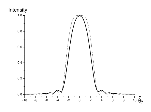


Now we can introduce the relative intensity
| (286) |
so that
| (287) |
and according to our approximations
| (288) |
With an obvious change of integration variable we finally obtain
| (289) |
It is now evident that similarity techniques we used are not only a theoretical tool: in fact is a universal function of and Eq. (289) can be integrated with the help of simple numerical techniques to get the universal plot in Fig. 15 (solid line). This universal plot is compared, always in Fig. 15 (dashed line), with the relative intensity in the case when also . In this case we simply have the single particle intensity
| (290) |
The dashed line in Fig. 15 refers to the case ; note the different normalization factor between and . It may be useful to provide a fit of the universal plot in Fig. 15 using the following function:
| (291) |
Fitting for , , , and and using, for instance, a reasonable value for we find , , , and which result in the solid curve in Fig. 16, the dashed curve being a comparison with the real universal function plotted in Fig. 15. It should be noted that has no particular physical sense: it simply gives an analytical approximation for the universal plot in Fig. 15 with graphical accuracy shown in Fig. 16.
After Fig. 15 is tabulated, one can plot the intensity as a function of for given values of simply solving for , being any of the tabulated abscissas with constraint . By fixing we obtain the universal plot in Fig. 17 (solid line). This universal plot is compared, always in Fig. 17 (dashed line), with the normalized intensity as a function of in the case when also . The dashed line in Fig. 17 refers to the case ; again, note the different normalization factor between and . Note that, for this case, Eq. (290) calculated for already constitutes a relatively good approximation for the plot in Fig. 17.
Letting vary we obtain universal plots of the intensity parameterized with respect to ; we show some of them in Fig. 18 and Fig. 19 with respect to and .
Finally, with the help of a Monte Carlo simulation described in more detail in the following Section V, we compared our results with the case of a beam with different values of and , always assuming and no energy spread is present. Note that in general, the spectrum (at ) or the angular intensity (at , ) is a function of two parameters: and . Results are shown in Fig. 20 and Fig. 21, where relative intensities are plotted as a function of for and and as a function of for and , respectively. Fig. 20 and Fig. 21 illustrate the accuracy of the asymptotic limit Eq. (289).


V Set of two undulators with a focusing triplet in between
In this Section we use our understanding of approximations and region of applicability discussed before to deal with a difficult setup constituted by two or more undulator segments separated by strong focusing quadrupoles. In this Section, and in Fig. 22, we consider the particular case of two undulator segments separated by a focusing triplet.

This scheme is known as segmented undulator scheme.
Insertion devices at PETRA III are due to work according to an on top injection scheme and must therefore be compatible with injection of new particles during operation. In general, injection operations require a larger beam acceptance with respect to an already circulating beam and this poses a strict limit to a safe choice of the length of the insertion devices.
Since no focusing element is present inside the undulator the function increases quadratically with the distance from the minimal value in the middle of the undulator. In practice, then, the maximal length of the insertion device is also fixed and one has the rule of thumb . Here we can safely talk about the vertical direction only, because the vertical function is also the shortest.
In principle, given a certain acceptance , it is possible to increase the -function by increasing the undulator gap according to . However, the particle energy and the radiation wavelength are nearly fixed at PETRA III. Moreover restrictions related with the number of photons required and with operation of third harmonic scheme apply, which allow only values of around unity. Then, is fixed as well as the magnetic field on axis and, as a result, the undulator gap too. This means that an upper limit on the function and therefore to the insertion device length is also fixed.
In practical situation, when enough experience with the machine, safety margins might be bent. For instance a single m-long in vacuum undulator operates at SPring-8 in on top injection mode with a vertical m. However, safety limits indicate, for a first design, much more stringent constraints.
For a first conservative design, the segmented undulator scheme constitutes a reliable alternative for filling the first straight section at the new arc of PETRA III, which can accommodate a m long insertion device. Breaking a long insertion device in several parts allows one to ”keep the average vertical -function rather small which in turn is essential to allow for a small geometrical vertical aperture and magnetic gap” (cited from PETR, Section 4.1.8). ”The maximal vertical -function along this undulator will be about m. Therefore a vertical inner size of mm is necessary for the corresponding chambers” (cited from PETR, Section 3.2.1).
With this motivation in mind we start our investigation. We are interested in computing the radiation intensity seen by an observer at angles and . We will be interested in both angular and spectral intensity distribution. Although it is possible to take advantage of the analysis performed in Paragraph IV.3 and treat near field effect, in this paper we will restrict our attention to the far field limit. Then we will compare our results with the case of an uniform undulator.
Of course radiation intensity can be obtained, numerically, from the Lienard-Wiechert expressions for the electromagnetic field without approximations of any kind. The previous statement though, sounds like declaring that solution to all electromagnetic problems can be found solving Maxwell’s equation: it is undoubtedly true, but quite generic. The most general expressions for the Lienard-Wiechert field can be used, and have been used (again, see CHUB and TANA for instance) as a basis for numerical codes, but understanding of correct approximations and their region of applicability can simplify many tasks a lot, including practical and non-trivial ones like the one we are going to study here. Instead of relying on computational power we propose a simple technique for dealing with the segmented undulator scheme which minimizes numerical difficulties and computation time and can be implemented straightforwardly also by non-expert programmers. In order to reach this result we will use our understanding of approximations in undulator radiation theory, thus simplifying equations as much as possible before using, in the final step, some numerical integration technique. It is worthwhile to stress the fact that we will have full control of our approximations at every step, meaning that we will be able to get the radiation intensity and the accuracy with which this is computed as well.
We will consider the undulators tuned at the fundamental frequency. Therefore we start reminding the resonant approximation seen in Section IV. In particular, using our method we were able to demonstrate that under the resonant approximation the field contribution from non-resonant structures can be neglected with respect to the undulator field with an accuracy of . Here we will restrict our attention to a region of parameters where such an approximation is valid. Having indicated, as in Fig. 22, with the straight section length, we will therefore be interested in the fundamental harmonic of the system within the assumptions: , , and .
Also, for the same reason and with the same accuracy we can neglect the constrained motion in the Green’s function phase and consider the particle moving on a straight line when calculating this phase term.
In Paragraph IV.4 we treated the case of a single electron with offset and deflection. If one is interested in the far field limit case, one can use Eq. (273) to obtain the contributions from each segment but special attention must be taken in summing up the fields with the correct relative phase factor.
With the help of Eq. (273) and the coordinate system depicted in Fig. 22 we start accounting for the field contributions from the first and the second undulator in the case there is no straight section between the two segments that is , defined as , is zero. In this case we have:
| (292) |
while
| (293) |
where
| (294) |
| (295) |
and
| (296) |
Here is defined as usual by Eq. (270); offsets refer to the middle point of the system (i.e. the point with zero value of in Fig. 22) and deflections and refer to the first and the second undulator respectively, and the relation between the two is determined by the focusing elements only: therefore it makes sense to talk about deflections for the first and the second undulator without specifying the point.
The next step is to account for the phase shift in the case . On the one hand, shifting the first segment of a quantity gives a phase contribution:
| (297) |
On the other hand, shifting the second segment of a quantity leads to an extra phase term:
| (298) |
To complicate the situation further, we should account for the fact that, in order to practically control the relative phase between the two contributions phase shifters will be installed. These devices are also useful in FEL technology (see PFLU); in the case of PETRA III, they will be usually designed and tuned in order to provide matching condition for particles at nominal energy moving at zero angle with respect to the undulator axis, and with zero detuning. This means that the phase shifter will contribute for a relative phase such that
| (299) |
where is an integer number. Taking out the unessential contribution (or setting ) and accounting for one gets
| (300) |
and
| (301) |
Finally, we make use of the relation and we express and in normalized units thus writing
| (302) |
and
| (303) |
where
| (304) |
We can account for a given energy deviation expanding around the nominal energy. Trivial calculations show that, for , being now calculated at and at nominal energy we obtain a shift in the detuning parameter given by
| (305) |
Including in our equations we obtain the final results:
| (306) |
and
| (307) |
with
| (308) |
| (309) |
| (310) |
| (311) |
where is now the detuning parameter for a particle with nominal energy and other quantities are as defined before.
As we have said, focusing elements simply change the electron trajectory, but they do not contribute directly to the total field at the observer position. We will treat them like a thin lens with focal length and in the horizontal and vertical planes respectively. We can, therefore, introduce normalized focal lengths and .
From now on, when possible, we will neglect indexes or for notational simplicity. If we have offset and deflection and at the entrance of the system (where , see Fig. 22), we can easily calculate
| (312) |
It is worth to note here that if we take the limit for and , the sum gives back Eq. (271), as it must.
Since we have many particles here we can consider a collective description of the beam, for instance in terms of the Twiss parameters , and for the horizontal and vertical planes at the entrance of the system, where . Knowing the Twiss parameters and the emittance at the entrance of the first undulator it is easy to write down the number of particles with offset between and and with deflection angles between and , always at the entrance of the system; in fact, one can simply write it as , where is the following density distribution ROSE:
| (313) | |||
| (314) |
Here is the number of particles in the beam and again, for notational simplicity, we are taking indexes and as implicit. Upon introduction of
| (315) | |||
| (316) | |||
| (317) | |||
| (318) | |||
| (319) |
we can write Eq. (314) as a function of dimensionless quantities as
| (320) | |||
| (321) |
| Quantity | Unit | Value |
|---|---|---|
| m | ||
| - | ||
| m | ||
| - | ||
| m | ||
| - | ||
| m | ||
| m-1 | ||
| m | ||
| m | ||
| - | ||
| m | ||
| m-1 | 0.260 | |
| m | ||
| m | ||
| - | ||
| - |
The local energy spread of the beam will be assumed to be a gaussian function with standard deviation :
| (322) |
where and
| (323) |
brackets indicating the ensamble average over the particle distribution.
A set of realistic normalized parameters for the segmented undulator is given in Table 1 and Table 2 for dimensional and dimensionless quantities, respectively. From these tables we can already foresee a large effect of the normalized energy spread parameter which is, in our case, comparable with the normalized horizontal emittance.
We can now average the normalized intensity over the particle distribution function and the energy spread of the beam at the entrance of the system thus finding the final expression for the total intensity
| (324) | |||
| (325) | |||
| (326) |
As in Eq. (284), the normalized intensity is related to the non-normalized intensity by
| (327) |
Moreover is expressed in terms of and in Eq. (312).
We now reached an expression, Eq. (326), which can be integrated with the help of numerical techniques. Results of numerical integration are the intensity as a function of the detuning parameter for fixed observation angles or the intensity as a function of angles for a fixed detuning parameter.
We developed a short code which uses a Monte Carlo method to compute Eq. (326). A quasi-random generator is used to fill the horizontal and vertical transverse phase space with a given number of particles. The actual simulation makes use of Sobol sequences to reduce the formation of cluster of particles, a well known phenomenon described, for instance, in REICH and references therein. Then, the intensity for each particle is calculated and all contributions are summed up to give an estimation of Eq. (326). The critical parameter in this kind of codes is the number of particles used. In general the higher the number of particles is, the smaller the fluctuation of the results from run to run and the higher the accuracy of the integration. On the other hand numerical algorithm designers warn that quasi-random sequences start to display unwanted correlations after several tens of millions calls to the generating routine. We observed that a choice of several million particles is more than sufficient to ensure that results converge fast enough so that no relevant fluctuation is present in the outcome (with graphical accuracy of the results which will be described in the next few figures).
First, we compared results from the Monte Carlo approach in the limiting case , , , and . Results were in perfect agreement with the ones shown in Fig. 15, Fig. 17, Fig. 18 and Fig. 19 as it should be. Then, as has already been said in Paragraph IV.4 we compared this asymptotic situation with a more practical case of a uniform undulator with and . Results have been already described, and shown in Fig. 20 and Fig. 21.


Finally we used all the features of our program in order to deal with the segmented undulator case. We set up parameters as in Table 1, which correspond to a design set for the PETRA III case. The solid line in Fig. 23 represents the intensity as a function of the detuning parameter at and . The dashed line in Fig. 23 is the intensity for the uniform undulator case, corresponding to the limit m and , while m. In this case we set the minimal betatron function values to m in the horizontal direction and m in the vertical one. Beam energy, wavelength, undulator deflection parameter, relative energy spread and electron beam emittances are left unvaried as in Table 1. Assuming the minimal function in the center of the undulator we can calculate the Twiss parameters at the system entrance using for both horizontal and vertical plane (see, for instance, ROSE) :
| (328) |
| (329) |
| (330) |
where indicates the -position at the beam waist, while subscripts ”o”, as usual, denote minimal values of the Twiss parameters. Taking m at the center of the system and m we obtain the initial Twiss parameters to enter in our program: , m and m-1, , m and m-1.
It is important to remark that we normalized the solid line in Fig. 23, that is the result for the segmented undulator, to the maximal intensity found for the uniform undulator while the dashed line represents the relative intensity for the uniform undulator. This allows direct comparison between uniform undulator and segmented undulator schemes.
To conclude, in Fig. 24 (solid line) we plot again the intensity as a function of at and . Similarly as for Fig. 23, the dashed line in Fig 23 represents a comparison with the uniform undulator case m and , where the other parameters are left unvaried as in Table 1. Normalization of the curves are as in Fig. 23. The final results for the two schemes do not appear to be dramatically different.
VI Conclusions
In this paper we have shown that even well-known and long studied subjects, like Synchrotron Radiation, continue to retain interest from a theoretical viewpoint. In particular we have proposed a technique to compute harmonic contributions of the electric field from a moving charge particularly suitable for analytical investigations. We showed that our general expression, Eq. (41), can be obtained from already known expression Eq. (7) with the use of a paraxial approximation, but also much more straightforwardly from Maxwell’s equation in paraxial form, with the help of a parabolic Green’s function method. The main advantage of our approach with respect to standard techniques is that we separated from very beginning approximations independent from the system under study (paraxial approximation) and assumptions that, from time to time, arise in the study of a particular magnetic system. This gave us the possibility to specify region of applicability and accuracy of well known results, which we were, of course, able to recover using our method, like the field from a charge moving on a circle, in a short bending magnet or in an undulator and also edge radiation effects from a particular setup. Again, our particular approach is logically much less involved with respect to the others, since it relies on direct integration of the paraxial Maxwell’s equations for a given harmonic. As a result, our expression gives a clearer and completely fresh insight in old results. Besides being able to discuss their region of applicability and their accuracy, we pointed out that phase corrections with respect to the spherical wavefront for an electron on a circle arise naturally from analytical treatment. We have seen that short magnet radiation is a complete separate phenomenon with respect to edge radiation. We stressed the importance of the knowledge of the entire electron trajectory in order to obtain a correct calculation of the field: from this viewpoint we have seen how edge radiation from two dipoles separated by a straight section arises, in our method, from the contribution due to the straight section alone, and that the field term from the magnets is completely negligible. We discussed, under resonance approximation, accuracy and applicability region of the far field undulator radiation and we dealt with near field effects as well: in particular we were able to reproduce already known results studying their region of applicability in detail, and we found also other regions of interest, where the near field parameter is of fundamental importance.
Besides this, our method proved to be a reliable basis for calculation of more complicated quantities like field autocorrelation functions, either from bending magnets or undulators, which are of fundamental importance in the understanding of spatial coherence properties of Synchrotron Radiation. In fact, by direct application of our general formula Eq. (41) we were able to provide analytically manageable expressions for bending magnet or undulator radiation in the case of an electron with a transverse offset and deflection. These expressions can be integrated over realistic beam particle distributions and can be used in very practical calculations. Their strength stems from the fact that they correctly account for the field phase and that they can be simply summed up to give results for apparently complicated situations. Complete treatment of spatial coherence would probably double the size of this paper. For this reason, this first work focuses on the basis of Synchrotron Radiation theory only.
A few applications which exploit the power of our approach have been selected for the final part of the paper. At the end of Section IV we addressed basic characteristics of undulator radiation in the presence of electron beam emittance. We discussed the asymptotic situation for a large horizontal and a small vertical emittance.
Finally, in Section V, we considered a novel undulator configuration (setup of two undulators separated by a focusing element) which is planned for installation at PETRA III. Computation of radiation characteristics from new setups by means of numerical techniques alone requires, almost always, modifications of existing simulation codes which can be better done by the code authors themselves. Up to date, the particular case we chose to study has not been included in existing simulation codes. For this reason we selected this particular example: our goal was to demonstrate that, in general, the application of our method allows solution of apparently difficult problems relying on simple computer algorithm which can be developed by non-expert programmers, with obvious advantages in saving time and better physical understanding.
We expect that our technique will be used in the future as a basis for developments of simulation codes and for physical understanding of complex situation as well.
VII Acknowledgements
The authors are grateful to Klaus Balewski, Werner Brefeld, Winfried Decking, Martin Dohlus, Hermann Franz, Petr Ilinski and Edgar Weckert for many useful discussions and to Oliver Grimm, Jochen Schneider and Ivan Vartanyants for their interest in this work.
References
- (1) J. Schwinger, Phys. Rev. 75, 1912 (1949)
- (2) D. Iwanenko and I. Pomeranchuk, Phys. Rev. 65, 343 (1944)
- (3) A. Sokolov and I. Ternov, Synchrotron radiation, Akademie Verlag, Berlin (1968)
- (4) J. Jackson, Classical Electrodynamics, John Wiley and Sons Inc. (1998)
- (5) H. Wiedemann, Particle accelerator physics, Springer-Verlag (1993)
- (6) H. Wiedemann, Synchrotron Radiation, Springer-Verlag, Germany (2003)
- (7) A. Hofmann, CAS - CERN Accelerator School 1998, CERN 98-04 (1998)
- (8) A. Hofmann, The physics of Synchrotron Radiation, Cambridge Univ. press, Cambridge (2003)
- (9) F. Ciocci, G. Dattoli et al., Insertion Devices for Synchrotron Radiation and Free Electron Laser, World Scientific Publishing Co. Pte. Ltd., Singapore (2000)
- (10) P. Duke, Synchrotron Radiation - Production and properties, Oxford University Press Inc., New York (2000)
- (11) PETRA III Technical Design Report, ISSN 0418-9833, edited by K. Balewski, W. Brefeld et al., DESY, Hamburg (2004)
- (12) H. Kitamura, T. Bizen et al., Nucl. Instr. Meth. Phys. Res. A, 467-468, 110 (2001)
- (13) T. Thurn-Albrecht, G. Meier et al., Phys. Rev. E 59, 642 (1999)
- (14) S. Mochrie, A. Mayers et al., Phys. Rev. Lett. 78, 1275 (1997)
- (15) O. Tsui and S. Mochrie, Phys. Rev. E 57, 2030 (1998)
- (16) D. Riese, W. Vos et al., Phys. Rev. E 61, 1676 (2000)
- (17) T. Seydel, A. Madsen et al., Phys. Rev. B, 63 0734099(4) (2001)
- (18) I. Sikharulidze, I. Dolbnya et al., Phys. Rev. Lett. 88, 115503(4) (2002)
- (19) A. Snigirev, I. Snigireva et al., Rev. Sci. Instrum. 66, 5486 (1995)
- (20) S. Wilkins, T. Gureyev et al., Nature 384, 335 (1996)
- (21) T. Gureyev, C. Raven et al., J. Phys. D 32, 563 (1999)
- (22) P. Cloetens, W. Ludwig et al., Appl. Phys. Lett. 75, 2912 (1999)
- (23) J. Miao, P. Charalambous et al. Nature 400, 342 (1999)
- (24) I. Robinson, J. Libbert et al., Phys. Rev. B 60, 9965 (1999)
- (25) J. Pitney, I. Robinson et al., Phys. Rev. B 62, 13084 (2000)
- (26) A. Letoublon, F. Yakhou et al. Europhyis. Lett. 54, 753 (2001)
- (27) O. Chubar, P.Elleaume et al., Nucl. Instr. Meth. Phys. Res. A, 435, 495 (1999)
- (28) T. Tanaka and H. Kitamura, J. Synch. Rad. 8, 1221 (2001)
- (29) O. Chubar, Rev. Sci. Instrum. 66, 1872 (1995)
- (30) O. Chubar and N. Smolyakov, Proceedings of the 1993 Particle Accelerator Conference, Washington DC, USA, 1626 (1993)
- (31) Y. Hirai, A. Luccio et al., J. Appl. Phys. 55(1), 25 (1984)
- (32) Y. Takayama and S. Kamada, Phys. Rev. E 59, 6 (1999)
- (33) V.G. Bagrov, N.I. Fedsov and I.M. Ternov, Phys. Rev. D 28, 2464 (1982)
- (34) G. Geloni, E. Saldin, E. Schneidmiller and M. Yurkov, DESY 03-031, ISSN 0418-9833, DESY, Hamburg (2003)
- (35) V. A. Bordovitsyn (Editor), Synchrotron Radiation Theory and Its Development, World Scientific, Singapure-London, (1999)
- (36) J. W. Goodman, Statistical Optics, John Wiley Sons, Inc., 1985
- (37) L. Mandel and E. Wolf, Optical Coherence and Quantum Optics, Cambridge University Press, 1995
- (38) D. Attwood, Soft X-rays and extreme ultraviolet radiation, Cambridge University Press, 1999
- (39) R.A. Bosch, Nucl. Instr. Meth. Phys. Res. A, 386, 525 (1997)
- (40) P. Roy, J-B. Brubach et al., Nucl. Instr. Meth. Phys. Res. A, 426 (2001)
- (41) R.A. Bosch, Nucl. Instr. Meth. Phys. Res. A, 482, 789 (2002)
- (42) P. Ilinski, Ph.D. Thesis, Illinois Institute of Technology (1998)
- (43) D. Alferov, Y.A. Bashmakov et al. Sov. phys. - Tech. Phys. 18, 1336 (1974)
- (44) R. Walker, Nucl. Instr. Meth. Phys. Res. A, 267, 537 (1988)
- (45) J. Pflüger and M. Tischer, TESLA-FEL 2000-08 (2000)
- (46) J. Rosenzweig, Fundamentals of beam physics, Oxford University Press Inc., New York (2003)
- (47) Y. Takayama, N. Takaya et al., Nucl. Instr. Meth. Phys. Res. A, 441, 565 (2000)
- (48) S. Reiche, Ph.D. Thesis, DESY-THESIS-2000-012, DESY, Hamburg (2000)