Instability of a moving contact line
Abstract
We study a solid plate plunging into or being withdrawn from a liquid bath, to highlight the fundamental difference between the local behavior of an advancing or a receding contact line, respectively. It is assumed that the liquid partially wets the solid, making a finite contact angle in equilibrium. In our hydrodynamic description which neglects the presence of the outer gas atmosphere, an advancing dynamic wetting line persists to arbitrarily high speeds. The receding wetting line, on the other hand, vanishes at a critical speed set by the competition between viscous and surface tension forces. In the advancing case, we apply existing matching techniques to the plunging plate geometry, to significantly improve on existing theories. For the receding contact line, we demonstrate for the first time how the local contact line solution can be matched to the far-field meniscus. In doing so, we confirm our very recent criterion for the instability of the receding contact line. The results of both the advancing and the receding cases are tested against simulations of the full model equations.
I Introduction
A number of recent experiments Q91; SP91; PFL01; SK03 have tested the stability of forced advancing and receding contact lines under conditions of partial wetting. For example, if a solid plate or fiber is plunging into a liquid bath to be coated (advancing contact line), the speed can be quite high (m/s) SK03, while maintaining a stationary contact line. In the opposite case of withdrawal (receding contact line) SP91, a stationary contact line is observed only for very low speeds, and a macroscopic film is deposited SP91; Q99 typically at a speed of only a few cm/s.
The description of a moving contact line is complicated by the fact that the Navier-Stokes equation with standard no-slip boundary conditions LL84 breaks down near it, because such a hypothetical flow would produce an infinite energy dissipation HS71. Instead, some microscopic length scale must be invoked that cuts off this singularity, which in this paper we are going to take as a slip length. As a result, the local flow near the contact line is characterized by a typical length of about a nanometer TR89, which has to be matched H to the macroscopic flow away from the solid. In this paper, we apply a matching method developed for spreading drops H83 to the plunging plate, and test the result by comparing to numerical simulations. This very significantly improves the results of earlier calculations for the same problem GHL90; H93. For the opposite case of a receding contact angle we find that a new matching procedure is needed. The results confirm our very recent criterion E042 for the instability of a receding contact line.


Figure 1 illustrates the geometry to be considered in the present paper. On the left, a solid plate is pushed into a pool of viscous liquid. As a result, the interface deforms and the contact line is pushed downward relative to its equilibrium position. Within the present model, this advancing contact line is stable at any speed. If the plate is withdrawn from the bath, fluid is pulled up with the plate, and a new contact line position is established. However, this state is realizable only at speeds below a critical speed . For the contact line is no longer sustainable and continues to move up the plate H01. In the stationary state, the plate is covered by a thin film, first described by Landau, Levich, and Derjaguin (LLD) LL42; D43. To understand the fundamental difference between pushing a plate and pulling it out, one has to consider the matching between the region very close to the contact line, and the capillary profile away from it. Qualitatively, the difference in the behavior of the advancing and of the receding contact line makes sense: if the plate is pushed into the liquid, the interface is bent away from the solid, and viscous forces are reduced. If the plate is pulled, the interface is pulled toward the solid, making the film thinner and enhancing viscous effects. Hence in the latter case there is a positive feedback increasing viscous forcing and thus leading to instability.
The strong energy dissipation near a moving contact line results from the fact that viscous forces become very large as the thickness of the liquid film goes to zero HS71. As a result of the interplay between viscous and surface tension forces, the interface is highly curved, and the contact line speed is properly measured by the capillary number , where is the viscosity of the fluid and the surface tension between fluid and gas. Owing to this bending the interface angle measured at, say, m away from the contact line differs G85; K93; FJ91; MGD93 significantly from the microscopic angle directly at the contact line.
The existence of a slip length , which is of the order of a few molecular diameters under normal circumstances TT97; CLR04; LRM04, implies a convenient separation of length scales between two different parts of the surface profile. On one hand, there is a contact line region whose typical scale is , on the other hand there is an “outer” meniscus region, whose typical length scale is set by the capillary length . Thus one expects the local “inner” behavior of the profile near the contact line to be of the form
| (1) |
since is the only available length scale. The dependence on the equilibrium contact angle was introduced for later convenience.
Firstly, one finds from (1) that the curvature of the interface is , which becomes large for as expected, while the slope is . The inner solution (1) has to be matched to an outer solution , whose curvature is of the order of , which means we have to join the two solutions at some scale with . This implies that the argument of can effectively be taken at , while . Thus the matching condition is
| (2) |
which ensures that the inner and the outer solutions are compatible. We will see that (2) needs to be supplemented by what is essentially a condition for the slope.
The matching condition (2) is the key to understanding wetting behavior. Let us summarize the main results of this paper by analyzing the solution qualitatively for the two cases of an advancing contact angle (plate plunging into the fluid) and of a receding contact angle (plate being withdrawn). For very small , it is clear that must be small for matching to be possible, so in the limit, becomes the boundary condition for the inner problem. We will see that for an advancing contact angle this boundary condition yields the inner scaling function , first found by Voinov V76. The matching to Voinov’s solution is slightly complicated by the presence of logarithmic terms in the slope H83.
On the other hand, Voinov’s solution cannot be applied to the case of a receding contact line. Rather, all inner solutions maintain a finite curvature . This means that at too small a value of the matching condition (2) can no longer be obeyed and the inner and the outer solutions are incompatible. As a result, the contact line vanishes. In a typical experiment, is constant and the speed is increased, but the effect is the same: since the curvature of the interface is caused by viscous forces HS71, increases with speed and matching becomes impossible. This explains the phenomenology described in Fig.1 above. The impossibility of matching a receding contact line above a critical capillary number was already noticed in V00, based on numerical integration of the thin-film equations. Analytical solutions for the inner solution will permit us to give a much more complete description.
In the next section we will introduce the hydrodynamic equations to be used for the calculation of stationary profiles. We will confine ourselves to the “lubrication approximation”, valid in the limit that the liquid film is thin. In the following section we consider the case of a solid plate being pushed into the liquid (advancing contact angle). By matching an inner to an outer solution, we compute the profile as a function of speed. In the fourth section we introduce the matching procedure for the opposite case of a plate being withdrawn (receding contact angle). The failure of this matching procedure gives the critical capillary number at which the contact line can no longer exist, in agreement with our earlier result E042. For speeds below the critical value we again find the interface profile. All our analytical results are tested by comparison with numerical solutions of the original equations. Finally, we summarize our results and indicate directions of future research.
II Lubrication description
As illustrated in Fig.1, we are considering a plate being pushed into or being withdrawn from a liquid bath at an angle . This means we have to solve the steady Navier-Stokes equation with a free surface, and no-slip boundary conditions on the plate. Since the plate is moving with speed U, the contact line between fluid, solid, and gas is moving relative to the solid. As explained above, the Navier-Stokes equation does not allow such a solution, and a small-scale cutoff has to be introduced at the contact line G85; K93. The dominant mechanism responsible for cutoff depends on the particular system under study K93; ES04. As a representative example, we assume that the corner singularity is relieved by allowing the fluid to slip across the solid surface, since the matching to the slip region of size is well understood in this case H83. According to the Navier slip law HS71, the fluid speed relative to the solid is proportional to the shear rate:
| (3) |
Recently, we found E041 that various modifications of (3) have a minimal influence on the interface away from the contact line. Hence we do not believe that the particular cutoff mechanism used is of great importance.
A much thornier issue is the slope of the fluid layer to be specified at the contact line. It is well appreciated that molecular processes are involved BH69; PRG99, which are beyond a hydrodynamic description. This will lead to a an effective speed dependence of the contact angle as defined on a scale of nanometers. The importance of these microscopic effects relative to hydrodynamic ones is determined by the amount of energy dissipation involved in either process BG92. Thus for high viscosities the speed dependence of the microscopic angle can most likely be ignored, in agreement with experimental data H75. If there is no “intrinsic” speed dependence of the microscopic angle, it must coincide with its equilibrium value at zero speed. We thus take .
The mathematical problem simplifies significantly if we assume that the angle the interface makes with the solid is always small, and that viscosity is sufficiently large for inertia to be ignored. In this limit, one can find an approximate description of the hydrodynamic equations which eliminates the flow field H83; H01, and the so-called “lubrication equation” can be written entirely in terms of the free-surface profile . Non-dimensionalizing all lengths with the capillary length one finds H01
| (4) |
where we consistently used the small-angle approximation . To distinguish more clearly between advancing and receding contact lines we always take as a positive quantity, and rather change the sign in the equation. The - sign corresponds to the plate plunging into the liquid, the + sign to the opposite case of the plate being withdrawn.
Viscous forces appear on the left of (4) (proportional to the speed), and diverge quadratically as goes to zero at the contact line. As a result, viscous dissipation would diverge if it were not for the presence of slip, which weakens the singularity. Near the contact line the surface is highly curved, so the first term on the right of (4), which comes from surface tension, balances the viscous term on the left. The other two terms stem from gravity and only come into play at greater distances from the contact line. The film thickness vanishes at the contact line, where the slope is as discussed above. Far away from the plate the surface coincides with the liquid bath, so the third boundary condition is . Rescaling the layer thickness with the equilibrium contact angle , one finds that there remain three parameters in the problem, namely the combinations , , and . However, we find it more intuitive to keep the original parameters, and to state results in terms of the above combinations if convenient.
III Pushing
We begin by considering a plate being pushed into a viscous fluid, corresponding to the - sign in (4). In the spirit of the matching condition (2) we approach this problem by first considering the leading-order behavior near the contact line, where goes to zero. As discussed above, this equation H83 is
| (5) |
which we studied in detail in E041 for a more general class of slip models. The characteristic scale of the local solution is the slip length , so it is convenient to introduce the scaled variables (1), which leads to
| (6) |
where is the rescaled capillary number.
As argued above, the matching condition (2) leads to the requirement that the curvature vanishes for large as the limit is performed. This means that the boundary conditions for the solution of (6) are
| (7) |
The only parameter now appearing in the problem is the rescaled capillary number , and equations (6)-(7) uniquely specify the profile close to the contact line.
This inner solution can be found by expanding in a power series in the capillary number in a manner described in many papers H83; H92; E041. If one writes the solution in terms of , its behavior for large can be written as
| (8) |
to any order in the capillary number E041. This is the form originally proposed by Voinov V76, using more qualitative arguments. The length appearing inside the logarithm can be computed as a power series in the capillary number:
| (9) |
but for simplicity we only take the leading order term into account here, as corrections introduced by the next order are usually quite small E041.
The crucial point of representing the inner solution in the form (8) is that the only parameter multiplying is the capillary number, which is defined in terms of the “outer” problem. Namely, the outer problem (8) needs to be matched to is
| (10) |
which does not contain any contact line parameters like or . Owing to the strong singularity for HS71; H83, (10) does not have a solution with finite slope at the contact line , making it impossible to impose a slope. Instead, we are seeking a solution of (10) that has the form (8) for , in other words
| (11) |
where is a constant to be computed. As demonstrated in H83, this can be achieved by expanding the outer solution in a power series in :
| (12) |
The equation for , representing a balance of surface tension and gravity, is
| (13) |
Equation (13) has the following family of solutions, which are finite at infinity and which vanish at the contact line:
| (14) |
The slope of (14) at the contact line is called the “apparent” contact angle and is a free parameter still to be determined by the matching procedure. Its name is motivated by the fact that a macroscopic measurement of the profile on the scale will yield a profile close to (14). If extrapolated to the contact line, the angle will appear to be , rather than the true microscopic value . Obviously, (14) cannot be matched directly to the contact line solution (8), which contains a logarithm. This logarithmic dependence will come out of the next-order solution , whose equation reads
| (15) |
The solution is straightforward BO78:
| (16) |
where once more any particular solution that is growing at infinity was suppressed, and are constants of integration. To find , we note that must vanish at the contact line, giving the first condition . To compute , we observe that the second integrand of (16) can be expanded like . The term linear in does not contribute for small , since behaves like for small arguments, and hence
Thus one finds
| (17) |
where the singularity of cancels out to make the second integral convergent.
Next we find a condition at infinity by noting that
| (18) |
where is vertical distance of the contact line from the undisturbed surface. Since we want to represent the far-field behavior of the profile, we put , and thus , by comparison with (14). This means we have
The first of the two terms on the right is zero, as one confirms by splitting it into two parts:
where is a large positive constant. The first of the two parts is evidently zero, for the second one notes that the argument can be approximated as for large , whose absolute value has the upper bound . Thus in the limit the second part vanishes as well. Using (17) this means the constant in (16) can be computed as
| (19) |
We are now in a position to determine the constant in (11). Comparing (11) to (12), we know that for small the first order contribution must have a logarithmic singularity of the form
| (20) |
Namely, for small
so that . Analysis of (16) for gives, using (19) and for small ,
| (21) |
This completely determines the the outer solution (12). Comparing it to the inner solution (8) we finally obtain
| (22) |
which is an equation to be solved for the apparent contact angle .

To test the result of our matching procedure (22), we compare the depression of the meniscus with the result of a numerical solution of the original equation (4). Remarkably, the prediction, which contains no adjustable parameters, remains extremely good up to a reduced capillary number of . To further appreciate the quality of the agreement, we plotted the result of an earlier theory GHL90 as the dotted line. In this earlier theory, a perturbation expansion of (4) in is matched directly to a linearized version of (8). However, the expansion is performed around the static profile corresponding to zero speed, whereas our expansion is around , which already incorporates a speed-dependent deformation of the surface. For the special case , the result of GHL90 is
| (23) |
where is Euler’s constant. A comparison of the profile obtained numerically with the outer solution (12) shows equally good agreement, as shown in Fig.3. It is only for that the outer solution begins to fail, since it has a logarithmic singularity at the origin.

IV Pulling
We now turn to the opposite case of a plate being withdrawn from a bath, for which the left-hand side of (4) is now positive. The dominant balance close to the contact line is again between the term on the left of (4) and the first term on the right. With the similarity transformation (1), this is converted into
| (24) |
which differs from (6) only by a sign. However, the behavior of solutions of (24) as is completely different. This is best appreciated by considering the form of (24) valid away from the contact line where :
| (25) |
where we have put .
Remarkably, this equation has an exact solution, whose properties have been summarized in DW97. In parametric form, a solution with reads
where and are Airy functions AS. The limit corresponds to , the opposite limit to , where is a root of the denominator of (IV):
| (29) |
Since the solution extends to , has to be the largest root of (29).
From (IV), the behavior of for large can be obtained DW97 (note that there is a misprint in equation (12) of DW97):
| (30) |
where
The constant can be determined by matching (IV), which is valid only for , to a solution of (24), which includes the effect of the cutoff and is thus valid down to the position of the contact line. The limit of (IV) for small values of gives DW97
| (31) |
which remains valid for . Thus, (31) is a valid solution of the full equation (24) for .
Following H83; E041, we compare (31) to the expansion of the full equation (24) in . Using the boundary conditions and , one finds
| (32) |
Since this solution has to match the logarithmic behavior (31), we put the constant of integration to zero, and (32) becomes for
| (33) |
Thus, comparing (33) to (31), we find
| (34) |
For , is indeed exponentially small, and (IV) has a logarithmic dependence over a large range of -values: . This makes it possible to match (IV) to (33) in the limit , although the ultimate behavior of (IV) for large is given by (30).
We are now in the position to match the inner solution of (24), which has the form (1), to an appropriate outer solution, following the prescription (2) given in the introduction. To achieve this matching it is enough to consider as given by (14), since (30) does not contain any logarithmic term. For , the solution of (24) is well described by (IV), so we have
| (35a) | |||
| (35b) | |||
where is given by (IV),(34). The matching procedure must supply us with the parameter in (IV), which is yet to be determined.
The matching works in the limit , for which we require that the expansions
agree, or
| (39a) | |||
| (39b) | |||
Eliminating between the two equations (39) we finally have
| (40) |
which should be read as an equation for . Once is known, all remaining parameters in and can be found. For example, from (39a) one finds the apparent contact angle to be
| (41) |
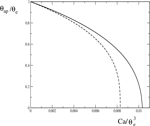
an example of which is plotted in Fig. 4. At some finite critical capillary number , goes to zero. Physical solutions cannot exist for capillary numbers beyond that, since the outer solution only makes physical sense for . Following E042, we now derive a much simpler equation for the critical capillary number at which the contact line disappears, and show that it is equivalent to .
Since , the maximum value of the left hand side of (39b), which is the curvature of the outer solution, is . The right hand side, corresponding to the curvature of the inner solution, is on the other hand bounded from below. From (30) it is seen that the minimum curvature corresponds to the condition that must be maximal among solutions of (29). By choosing we can in fact ensure that assumes its global maximum , which occurs for . Thus we have singled out a unique solution of (25) which minimizes the curvature
| (42) |
the value of which increases with capillary number as expected.
Now by equating the maximum value of the left hand side of (39b) with the minimum value of the right of (39b) we obtain an equation for a capillary number above which no solution can exist: , or explicitly
| (43) |
But at the capillary number given by (43), the first matching condition (39a) is also satisfied identically, since . This is because is extremal, so . Thus as given by (43) gives exactly the critical capillary number corresponding to in Fig.4. This confirms a classical conjecture by Derjaguin and Levi DL64, later reiterated by others BR79, that the transition to a film is characterized by the apparent contact angle going to zero. This criterion was confirmed experimentally in SP91, using fibers being pulled out of a viscous liquid.

The concept underlying equation (43) for the critical capillary number is illustrated again in Fig.5. Below the critical capillary number, there is some overlap in the curvature of the inner and the outer solutions (left diagram in Fig.5). The matching equation (40) determines which solution is selected from this overlap region. Above the critical capillary number, there can be no solution (right diagram in Fig.5): there is no outer solution which could be matched to an inner solution, because this would result in a sudden jump in the curvature.

In Fig. 6 we show the result of a numerical integration of (4) at the critical capillary, and compare it to the inner and outer solutions (35). The critical capillary number was found numerically by raising until no more solutions of (4) could be found. For large , the slope of the outer solution (35a) agrees with the numerical solution, but extrapolates to at the contact line, as reqired by . Coming from the interior, the inner solution (35b) agrees with the full solution up to the turning point.
To obtain a profile that is more uniformly valid, one can use a composite approximation H. The idea is to add the inner and outer solutions that have been matched, and to subtract the behavior (IV) in the region in which the two solutions overlap:
| (44) |
It is evident that agrees with the full solution for large as well as for small , hence it will be the best global approximation at this order of the matching. This excludes the region where (35b) has a logarithmic singularity. Figure 7 illustrates the remarkable agreement of the composite solution with the full numerical result at the critical capillary number, where the approximation is expected to be worst.

Having studied the critical capillary number, let us return once more to the matching condition (40) which determines the solutions for . Namely, it is instructive to obtain explicit solutions of (40) in the limit of small , in which case its solution is large, and the asymptotics of the Airy function AS gives
| (45) |
Thus, (40) becomes for small :
| (46) |
and (41) is
| (47) |
In the simplest approximation the exponent in (46) must vanish, , and inserting this into (47) gives . Not surprisingly, at very small capillary numbers the interface is hardly deformed at all.
To go beyond this approxiamtion, we put , insert into (46), and analyze the result for small , which gives
Putting this into (47) leads to the next approximation
| (48) |
which is similar to equation (22) for the apparent contact angle in the advancing case. Indeed, for small capillary number (22) becomes
| (49) |
which has the same form as (48). However, even for small capillary number the receding and the advancing case needs to be treated differently, as the constant inside the logarithm is different. For the argument of the logarithm in (48) becomes singular, which means one has to go to an even higher order in the approximation, but we are not pursuing this special case here. The approximation (48) is plotted as the dashed line in Fig.4. If extrapolated naively to , it gives a surprisingly good estimate of .
V Discussion
Let us begin by considering rather straightforward extensions and generalizations of the present theory. Firstly, our arguments are not limited to a specific contact line model, since they are based entirely on hydrodynamic arguments away from the contact line. For example, if van-der-Waals forces are dominant near the contact line GHL90, this only changes the parameter appearing in (8) (advancing contact angle) or in (31) (receding contact line). In the latter case, the slip length in (43) has to be replaced by , where is the Hamaker constant. Our research also suggests that the calculation of the critical capillary number is captured fully by lubrication theory, even if is not small. In that case the flow directly at the contact line would have to be described without resorting to lubrication theory V76; C86, but the relevant region where matching occurs is characterized by slopes which are small.
Secondly, one can generalize to a different geometry. To this end one has to replace (14) by the appropriate static solution for the problem at hand. This is done almost trivially for the case of a vertical plate or a fiber LL84, in which case the lubrication description (4) is no longer valid far from the contact line, since is not small. This however does not pose a problem since this part of the profile is determined by surface tension and gravity alone. In the same spirit, the present model can be exteded to a flow inside a capillary tube, with only very minor changes to the value of the critical capillary number H01.
Thirdly, one can consider dynamical effects, of particular interest for the unstable case of a receding contact line. In H01 it was found that when the stationary profile vanishes, it is not followed directly by the LLD film, which is of macroscopic thickness. Rather, there is a narrow range of speeds where the contact line is pulled up the plate, but at a speed that is smaller than , i.e. the contact line is partially slipping. The thickness of the film that is left behind is in the order of , i.e. microscopic. Only when the speed is raised still further does the LLD film appear. So far these results are only numerical; a full analytical theory would be desirable. Note also that these transitions are strongly hysteretical. Once the LLD film has appeared, it can be sustained to much lower capillary numbers than . It is usually assumed that the LLD film vanishes when its thickness has reached the range of intermolecular forces Q99, but we are not aware of any theoretical investigation of this problem.
Next we come to the experimental evidence. The most extensive experiments on the critical capillary number for a receding contact line were done with a capillary tube Q91, by pushing out a viscous liquid. Using a variety of different materials it was found that instability occurs at a given value of the reduced capillary number , in agreement with the present theory. The actual value of the critical capillary number, however, is about a factor of two too low, if the theoretical estimates are based on nm. Several possible explanations suggest themselves. First, the materials used in Q91 have considerable contact angle hysteresis, pointing to surface roughness. This will tend to reduce the critical capillary number GR01; GR03. In addition, any speed dependence of the microscopic contact angle, neglected in the present description, will effectively lower and thus lead to a smaller critical capillary number.
Our theory for the vanishing of the receding contact line has some similarities with an earlier theory G86, in that the critical capillary number is proportional to (cf. (43)). However, it differs in predicting a vanishing apparent contact angle at the transition, while it is in G86. The approach of G86 is also different in that it considers the local problem in isolation, hence the dependence of on parameters of the outer problem like cannot be captured. In fact, we believe that the mechanism for instability proposed in G86, which is based on an approximate solution of (24), contains a flaw. In E041 we use the case of the advancing contact angle (6) to show that the method of solution proposed in G86 cannot correctly predict the nonlinear dependence of the angle on speed. But it is precisely this nonlinear dependence which lies at the heart of the stability analysis of G86.
The most important extension of the present theory of contact line instability however is its application to higher dimensions, in which the contact line no longer remains straight. If the plate withdrawn from the liquid bath is sufficiently wide, the contact line inclines relative to its direction of motion. Two sections of the contact line that have inclined in opposite senses meet at a sharp corner, so that the whole contact line is serrated in an irregular fashion BR79.
A more controlled recent experiment is that of a viscous drop running down an inclined plane PFL01. At a critical speed, the initially rounded tail of the drop forms a sharp corner. A recent theory LS04 explains the drop profile near the corner of the drop, but not the critical speed at which the the corner first occurs, nor its opening angle. To give a complete description of the transition, the microscopic neighborhood of the contact line has to be included, as was done in the present theory for a straight contact line. One important difference between the case of a sliding drop and that of the present paper is that recent experimental evidence suggests that the transition occurs at a finite value of the apparent contact angle L04. Studies to understand the three-dimensional instability of a sliding drop are currently under way.
Acknowledgements.
I am grateful to Martin Sieber for several important discussions on the matching procedure, to Seth Lichter for improving my physical understanding, and to Lorena Barba for a careful reading of the manuscript.References
- (1) D. Quéré, On the minimal velocity of forced spreading in partial wetting. (in French) C. R. Acad. Sci. Paris, Série II 313, 313 (1991).
- (2) R.V. Sedev and J.G. Petrov, The critical condition for transition from steady wetting to film entrainment. Colloids and Surfaces 53, 147 (1991).
- (3) T. Podgorski, T., J.M. Flesselles, and L. Limat, Corners, cusps, and pearls in running drops. Phys. Rev. Lett. 87, 036102 (2001).
- (4) P. G. Simpkins and V. J. Kuck, On air entrainment in coatings. J. Col. Interf. Sci. 263, 562 (2003).
- (5) D. Quéré, Fluid coating on a fiber. Ann. Rev. Fluid Mech. 31, 347 (1999).
- (6) L.D. Landau and E.M. Lifshitz, Fluid Mechanics, Pergamon, Oxford (1984).
- (7) C. Huh and L. E. Scriven, Hydrodynamic model of steady movement of a solid/liquid/fluid contact line. J. Coll. Interf. Sci. 35, 85 (1971).
- (8) P.A. Thompson and M.O. Robbins, Simulations of contact-line motion: slip and the dynamic contact angle. Phys. Rev. Lett. 63, 766 (1989).
- (9) E.J. Hinch, Perturbation methods, Cambridge, 1991.
- (10) L. M. Hocking, The spreading of a thin drop by gravity and capillarity. Q. J. Appl. Math., 36, 55 (1983).
- (11) P. G. de Gennes, X. Hua, and P. Levinson, Dynamics of wetting: local contact angles. J. Fluid Mech. 212, 55 (1990).
- (12) L.M. Hocking, The influence of intermolecular forces on thin fluid layers. Phys. Fluids A 5, 793 (1993).
- (13) J. Eggers, Hydrodynamic theory of forced dewetting. Phys. Rev. Lett. 93, 094502 (2004).
- (14) L.M. Hocking, Meniscus draw-up and draining. Euro. J. Appl. Math. 12, 195 (2001).
- (15) L.D. Landau and B.V. Levich, Dragging of a liquid by a moving plate. Acta physico-chimica USSR 17, 42 (1942).
- (16) B.V. Derjaguin, On the thickness of a layer of liquid remaining on the walls of vessels after their emptying, and the theory of the application of photoemulsion after coating on the cine film. Acta physico-chimica USSR 20, 349 (1943).
- (17) P.G. de Gennes, Wetting: statics and dynamics. Rev. Mod. Phys. 57, 827 (1985).
- (18) S. Kistler, Hydrodynamics of wetting. In Wettability, J. C. Berg (Ed.), Marcel Dekker, New York (1993).
- (19) M. Fermigier and P. Jenffer, An experimental investigation of the dynamic contact angle in liquid-liquid systems. J. Coll. Interf. Sci. 146, 226 (1991).
- (20) J.A. Marsh, S. Garoff, and E.B. Dussan V., Dynamic contact angles and hydrodynamics near a moving contact line. Phys. Rev. Lett. 70, 2778 (1993).
- (21) P.A. Thompson and S.M. Troian, A general boundary condition for liquid flow at solid surfaces. Nature 389, 360 (1997).
- (22) J.-H.J. Cho et al., Dipole-dependent slip of Newtonian liquids at smooth solid hydrophibic surfaces. Phys. Rev. Lett. 92, 166102 (2004).
- (23) S. Lichter et al., Mechanism for liquid slip at solid surfaces. Phys. Rev. Lett. 93, 086001 (2004).
- (24) O. V. Voinov, Hydrodynamics of wetting. [English translation] Fluid Dynamics 11, 714 (1976).
- (25) O.V. Voinov, Wetting: Inverse Dynamic Problem and Equations for Microscopic Parameters. J. Colloid Interf. Sci. 226, 5 (2000)
- (26) J. Eggers and H. A. Stone, Characteristic lengths at moving contact lines for a perfectly wetting fluid: the influence of speed on the dynamic contact angle. J. Fluid Mech. 505, 309 (2004).
- (27) J. Eggers, Toward a description of contact line motion at higher capillary numbers. Phys. Fluids 16, 3491 (2004).
- (28) T.D. Blake and J.M. Haynes, Kinetics of Liquid/Liquid Displacement. J. Colloid Interface Sci. 30, 421 (1969)
- (29) A. Prevost, E. Rolley, and C. Guthmann, Thermally activated motion of the contact line of a liquid Helium-4 meniscus on a Cesium substrate. Phys. Rev. Lett. 83, 348 (1999).
- (30) F. Brochard-Wyart & P.G. de Gennes, Dynamics of partial wetting. Adv. Colloid Interface Sci. 9, 1 (1992).
- (31) R.L. Hoffman, A Study of the Advancing Interface. J. Coll. Interf. Sci. 50, 228 (1975).
- (32) L.M. Hocking, Rival contact-angle models and the spreading of drops. J. Fluid Mech. 239, 671 (1992).
- (33) C.M. Bender and S.A. Orszag, Advanced mathematical methods for scientists and engineers, Mc Graw-Hill, New York (1978).
- (34) B.R. Duffy and S.K. Wilson, A third-order differential equation arising in thin-film flows and relevant to Tanner’s law. Appl. Math. Lett. 10, 63 (1997).
- (35) B.V. Derjaguin and S.M. Levi, Film coating theory, Focal Press, London (1964).
- (36) T. D. Blake and K.J. Ruschak, A maximum speed of wetting. Nature 282, 489 (1979).
- (37) Abramowitz, M., Stegun, I.A., Handbook of Mathematical Functions, (Dover, 1968).
- (38) R.G. Cox, The dynamics of the spreading of liquids on a solid surface. Part 1. Viscous flow. J. Fluid Mech. 168, 169 (1986).
- (39) G. Golestanian and E. Raphaël, Relaxation of a moving contact line and the Landau-Levich effect. Europhys. Lett. 55, 228 (2001).
- (40) G. Golestanian and E. Raphaël, Roughening transition in a moving contact line. Phys. Rev. E 67, 031603 (2003).
- (41) P. G. de Gennes, Deposition of Langmuir-Blodget layers. Coll. Pol. Sci. 264, 463 (1986).
- (42) L. Limat and H.A. Stone, Three-dimensional lubrication model of a contact line corner singularity. Europhys. Lett. 65, 365 (2004).
- (43) L. Limat, private communication (2004).