B.S. Physics and Mathematics
Stanford University, 1995
\departmentDepartment of Physics
\degreeDoctor of Philosophy
\degreemonthFebruary
\degreeyear2002
\thesisdateFebruary 6, 2002
Michael S. FeldProfessor of Physics
Thomas J. Greytak
Professor of Physics
Associate Department Head for Education
Multiple Thresholds and Many-Atom Dynamics in the Cavity QED Microlaser
This thesis describes a study of a cavity QED microlaser in which many atoms are present simultaneously and atom-cavity interaction is well-defined. The microlaser is found to display multiple thresholds analogous to first-order phase transitions of the cavity field. Hysteresis is observed as a function of atom-cavity detuning and number of atoms. Data is compared with a rate equation model and fully quantized treatment based on micromaser theory. Good agreement between theory and experiment is found when the cavity is resonant with atoms of the most probable velocity, but long lifetimes of metastable states preclude the observation of true steady-state transition points. For nonzero atom-cavity detuning the microlaser displays broadenings and shifts which are not yet well-understood.
Quantum trajectory simulations are performed to investigate many-atom and finite transit time effects in the microlaser. We show that over a wide range of parameters the many-atom microlaser scales with the single-atom theory, with a perturbation in the photon statistics due to cavity decay during the atom transit time.
Acknowledgments
It is a pleasure to thank the many people who contributed directly or indirectly to this work. First I thank Michael Feld for his guidance and support during my time as a graduate student. His intuitive approach to physics and optimistic attitude will be an inspiration to me for years to come. I also appreciate the freedom he has given me as a graduate student to set the direction for my research.
This thesis would not have been possible without Kyungwon An, who initiated the microlaser experiment as a graduate student. Kyungwon taught me a great deal about experimental physics during my early years at MIT.
An equally large amount of credit for this thesis should go to Chung-Chieh Yu, who worked on the project for three years. His expertise in quantum optics and atomic beams helped move the project along faster than ever before.
Ramachandra Dasari deserves thanks for many useful discussions, and for managing lab equipment and funding issues. From the beginning Ramachandra expressed confidence in me and my ability to eventually take on a leading role in the project. This is something I have appreciated very much.
I enjoyed working with several other students in the laboratory. Abdulaziz Aljalal developed the optical velocity selection scheme and second-order correlation experiment. Bryndol Sones performed the absorption-induced bistability experiments. Alan Heins helped construct the dye laser locking system and the supersonic oven. Sangkeun Ha designed several of the electronic circuits and assisted with data collection.
Professor John Thomas of Duke University deserves special thanks for helping us develop the supersonic beam oven that has proved critical to the success of these experiments.
Thanks to Steve Smith of Coherent who often went out of his way to keep the laboratory equipped with working lasers.
I thank the members of my thesis committee, Marlan Scully, Daniel Kleppner, and Erich Ippen, for their helpful questions and suggestions.
This research was funded by a grant from the National Science Foundation. My research assistantship has been supported by a Lester Wolfe Fellowship.
Thanks to all my previous teachers and mentors who have inspired me to pursue a career in science, especially David Witt, Michael Russelle, Doug Osheroff, and Mark Dykman.
I dedicate this thesis to my parents, John and Rosemay.
C. F. Y.
Chapter 1 Introduction
1.1 Cavity QED and the microlaser/micromaser
One of the simplest models for light-matter interaction consists of a single two-level atom interacting with a single electromagnetic field mode of a cavity. If the atom-cavity coupling is stronger than the atomic or photon decay rates, the irreversible decay of an excited atom is replaced by an oscillatory exchange of energy between the atom and cavity, in a manner characteristic of two coupled oscillators.
In the 1950’s this model was the subject of considerable theoretical study, primarily in connection with the then-recently invented maser [1]. Experimental realization of such a strongly coupled system would not occur until several decades later, however, with advances in Rydberg states and superconducting microwave cavities.
In the early 1980’s the micromaser, or single-atom maser, was invented by Walther and collaborators [2]. In this experiment, individual Rydberg atoms pass through and emit photons into a superconducting microwave cavity with extremely high quality factor. The micromaser formed a close approximation to the single-atom, single-mode ideal. Subsequent experiments showed that the micromaser exhibited a variety of interesting and unusual phenomena, including trap states, near-number states, bistability, and nonclassical statistics [3]-[7].
The recent development of multilayer dielectric mirrors with very low loss has made it possible to conduct similar experiments at optical wavelengths. In 1994 Kyungwon An and Michael Feld developed the microlaser, the optical analogue of the micromaser [8, 9]. This device is also known as the cavity QED microlaser in order to distinguish it from other microlasers, for example those using semiconductor microresonators.
This thesis describes the first experiments exploring the microlaser’s truly unusual properties. In particular, we show that in contrast to conventional lasers which display a single laser threshold, the microlaser exhibits multiple thresholds.
1.2 Microlaser concept
The basic scheme of the microlaser is illustrated in Fig. 1.1. A beam of two-level atoms pass through a resonant high-finesse optical cavity. Before entering the cavity mode each atom is excited to its upper state via a laser -pulse. The atom interacts with the mode for a time , during which it may emit a photon into the cavity.
The key characteristic of the microlaser is not only the strong atom-cavity coupling but that different atoms experience almost the same interaction with the cavity: both the atom-cavity coupling strength and the atom-cavity interaction time are well-defined. It will be shown in chapter 2 that the resulting emission probability can be written as
| (1.1) |
where is the number of photons present in the cavity prior to the entrance of the atom. The unusual properties of the microlaser are primarily due to this sinusoidal dependence of the atomic emission probability on the cavity photon number.

1.3 Previous work
1.3.1 Micromaser
Reviews of the micromaser can be found in a number of references in the bibliography. Most relevant for this experiment is the study by Benson et al [11] of dynamic behavior near the micromaser field phase transitions. Spontaneous jumps and slow transitions between metastable states are observed; hysteresis is seen as interaction times are varied. The results were explained by quantum Monte Carlo simulations and a Fokker-Planck description of the micromaser dynamics. The presence of small stray fields prevented a full quantitative agreement between theory and experiment from being reached; the calculated transition rates were generally much slower than what was observed experimentally.
1.3.2 Microlaser vs. micromaser
We comment here on how the microlaser differs from its microwave counterpart.
Many atoms required
The threshold atom number as derived in Chapter 2 is
| (1.2) |
For our current microlaser with supersonic beam we have , , and , giving .
This is to be compared with the micromaser for which typical figures are Hz, , and kHz (values from [11]), so threshold atom number , almost five orders of magnitude lower.
One consequence of the many-atom nature is that the trap state resonances, corresponding to situations in which atoms perform an integer number of entire Rabi oscillations, cannot observed; nor can the associated near-number states of the micromaser [7]. However, other interesting effects appear from the many-atom case. The many atom nature of the current microlaser is treated in detail in Chapter 3.
No thermal photons
At finite temperature every field mode has a nonzero photon occupancy given by the Planck formula. For the micromaser operating at GHz, blackbody photons is as high as 0.15 even at 0.5 K and have a significant effect on the micromaser, as discussed in many micromaser articles. In the microlaser at 300K, and can be ignored.
Constant transit time
Micromaser experiments are typically performed with a fixed atomic injection rate and variable interaction times. This roughly corresponds to varying the pump parameter as described in micromaser theory (see Chapter 2).
Use of a supersonic beam of the microlaser prevents any significant variation in the transit times. Instead, the parameter most easily varied is the number of intracavity atoms . As is varied, both the expectation photon number and the pump parameter change.
Direct detection of photons
Optical frequency photons can be easily outcoupled out of a cavity, and have sufficiently high energy to be directly individually via a photomultiplier tube or avalanche photodiode. This is in contrast to the micromaser experiments, in which maser oscillation must be inferred via observation of the atom states. Direct detection of photons opens up new possibilities for photon statistics or laser linewidth experiments.
Atom-cavity coupling
The centimeter-scale wavelengths used in the micromaser allow the atomic beam to largely avoid coupling nonuniformities due to mode structure. In the micromaser, standing-wave coupling variation requires us to employ a traveling-wave interaction scheme (see Chapter 4). In addition, the small dimensions of the cavity mode and requirement of uniform coupling place strict requirements on the position and geometry of the atomic beam coupled to it.
1.3.3 Optical cavity QED
At optical wavelengths the experiments most similar to this one have been spectroscopy and probe transmission experiments of high-finesse optical cavities containing a small number of atoms.
Heinzen and Feld [12, 13] performed the first observation of enhanced and supressed spontaneous emission and level shifts in an optical cavity.
The vacuum normal-mode splitting of atoms in a cavity was observed in [14].
Oscillatory transmission and nonclassical photon statistics of a probed cavity was reported by the Kimble group [15]. Optical bistability was also observed.
To our knowledge, all these optical experiments employed atomic excited states with lifetimes ns much shorter than atom-cavity transmit times. They were performed in passive (non-laser) cavities in which a probe beam was incident. In addition, the atom-cavity couplings were not well-determined due to standing-wave mode profiles (cf. chapter 4).
1.3.4 Lasers and optical bistability
Bistability in the microlaser bears some similarity to “classical” optical bistability (see, for example, [16]) in active and passive cavities. Multimode laser bistabilities due to mode competition in gas lasers have been studied since the earliest days of the laser [17]. Current-feedback bistability has been observed in some semiconductor laser systems, e.g. [18].
1.3.5 Phase transition analogies
A detailed description of a laser is necessarily statistical in nature, due to the presence of randomness in many forms and large numbers of degrees of freedom. It is therefore natural to draw analogies between laser behavior and other problems in statistical physics. In particular, for some time physicists have drawn analogies between a laser near threshold and matter near a second-order phase transition. This comparison was first described in detail by DeGiorgio and Scully in 1970 [19, 20], although mention of this analogy date back considerably earlier (cf. references in ibid.).
In the present work we investigate jumps in the microlaser field which can be shown to be analogous to first-order (discontinuous) phase transitions [21]. To our knowledge no similar behavior has been observed in any other laser.
1.3.6 Many-atom dynamics in cavity QED
The field of collective effects in radiative properties goes back at least to Dicke [22], who showed that a collection of two-level radiators, localized within a distance smaller than their radiative wavelength, may emit photons at a collective rate that scales with instead of the usual .
Many-atom effects in the micromaser have been studied by a number of authors ([23]-[25]). It is well-known that the micromaser’s trap state resonances are easily destroyed by two-atom events ([26] and [27]).
A study by Kolobov and Haake [23] of two-atom events predicts a change in average photon number as well as location of the first-order thresholds, relative to the single-atom theory. On the other hand, Elk [24], considers a micromaser injected with multiple atoms, equally spaced in time, and finds a scaling behavior very similar to the single-atom theory. D’Ariano [25] considered a micromaser pumped with clusters of up to several hundred atoms at once, an interesting model but one that cannot be considered realistic in the present context.
Chapter 2 Theory of the microlaser
We begin by considering the ideal model of a single atom in a cavity. The microlaser is introduced by an semiclassical rate equation model which describes the basic features of the microlaser in an intuitive way. We then give a fully quantized treatment following the density matrix approach [28]. A Fokker-Planck analysis from [21] is reviewed which reproduces the rate equation solutions and also describes the transitions between different solutions in terms of an effective potential.
2.1 Atom in a cavity
The Hamiltonian describing the interaction of a radiation field with a single-electron atom is
| (2.1) |
where and are the atom and radiation field energies, is the position of the electron, and is the electric field operator:
| (2.2) |
| (2.3) |
| (2.4) |
Here the sum is over all allowed wave vectors and
| (2.5) |
is a function of mode volume which for a near-planar cavity is given by
| (2.6) |
where is the cavity mirror separation and is the Gaussian mode waist at the center of the cavity.
The atom-field interaction is given by
| (2.7) |
where
| (2.8) |
For a two-level atom, we have in the rotating-wave approximation (i.e. neglecting non-energy-conserving processes)
| (2.9) |
where , are photon creation and destruction operators, , are atom creation and destruction operators, is the atom level spacing.
For a single mode cavity of frequency we have
| (2.10) |
To go to the interaction picture we write
| (2.11) |
The Hamiltonian in the interaction picture is
| (2.12) |
where is the atom-cavity detuning.
| (2.13) |
The atom-cavity wavefunction can be written
| (2.14) |
where corresponds to a state with an excited atom with photons in the cavity, etc. Clearly the Hamiltonian mixes only the states and . Therefore the Schrodinger equation can be written as the coupled equations
| (2.15) |
| (2.16) |
A general solution is given by
| (2.17) |
| (2.18) |
where
| (2.19) |
If the atom is initially in the excited state, then and , and
| (2.20) |
| (2.21) |
Consider the case of perfect resonance and initial condition of excited atom with exactly cavity photons. The solution is then given by
| (2.22) |
| (2.23) |
with all other , equal to zero.
2.2 Rate equation for microlaser
Equations 2.22 and 2.23 describe resonant quantized Rabi oscillation. Note that oscillation proceeds even for an initially empty cavity () (vacuum Rabi oscillation).
In the microlaser, atoms interact with the cavity for an interaction time . The emission probability for an atom is given by the squared ground state amplitude after its interaction with the cavity:
| (2.24) |
where for simplicity we suppose that the cavity initially contained exactly photons.
Let us now write a rate equation for the cavity photon number : the time rate of change of is equal to to the difference between gain and loss terms:
| (2.25) |
which is set equal to zero at steady-state. Here is the number of atoms in the cavity, which can be defined by , the injection rate. Loss is equal to the photon number multiplied by the cavity loss rate .
The rate equation can be solved graphically as in Fig. 2.1. In general there exists more than one solution.
A solution is called stable if the system responds to a small perturbation in in a manner that tends to restore the original solution.
| (2.26) |
In terms of Fig. 2.1 a solution is stable if and only if the slope of the loss line exceeds that of the gain line at their intersection.

photon number
The threshold atom number is given by the point at which the gain and loss terms have equal slope, assuming small argument of the sine function:
| (2.27) |
Solutions to 2.25 as the injection rate is varied are plotted in Fig.2.2 , with . The number of solutions increases indefinitely with increased . Solutions are asymptotic to constant- lines corresponding to integer number of Rabi oscillations , integer.
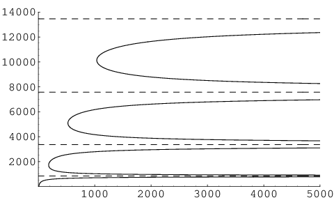
The rate equation analysis shows how the atoms’ sinusoidal emission probability leads to bistability and multistability. However, its derivation was less than rigorous and assumes that the cavity photon number is well-determined. In addition, it gives no information about the relative stability of different solutions, or the cavity photon statistics.
For a more complete theory we turn to the quantum theory developed for the micromaser by Filipowicz, Meystre, Scully and others ([21])
2.3 Quantum theory of microlaser
We follow the density matrix approach [28]. This theory in based on the following assumptions:
- 1.
Excited atoms are injected at a rate low enough so that at most one atom at a time is present in the cavity.
- 2.
Excited and “ground” state lifetimes are much longer than .
- 3.
Cavity damping during interaction time is small:
2.3.1 Density matrix equation of motion
Gain term
Consider the change in the cavity field density matrix due to the injection at time of an excited atom, which then interacts with the cavity for time :
| (2.28) |
The state may be found by determining the atom-field evolution from time to and then tracing over atomic variables:
| (2.29) |
Note that density operators with four indices represent combined atom-cavity systems; those with two represent the field only. A coarse-grained derivative for the gain contribution to the field density matrix can now be written
| (2.30) |
We now replace with the arbitrary continuous time . The time-evolved density matrices and are determined from the solutions for the excited state amplitudes as in section 1 of this chapter. We have
| (2.31) |
which gives for the density matrices
| (2.32) |
We then have the reduced field density matrix equation of motion:
| (2.33) |
Note that we have made no assumptions about the photon number distribution
Loss term
The contribution due to cavity loss is
| (2.34) |
for zero thermal photons. This is a standard result from the theory of oscillators coupled to a reservoir (c.f. [28] chapter 8.)
2.3.2 Steady-state photon statistics
Setting gives the equation
| (2.39) |
which leads to the following recurrence relations:
| (2.40) |
| (2.41) |
We obtain the steady-state photon distribution of the microlaser:
| (2.42) |
where is determined from normalization.
| (2.43) |
It is convenient to define two quantities, the expectation photon number
| (2.44) |
equal to the number of atom injections per cavity decay time, and the normalized interaction time or pump parameter
| (2.45) |
which is the Rabi phase if photons are present. Linearization of the rate equation for small and setting gain equal to loss gives as the laser threshold condition.
Mean photon number
In Fig. 2.3 the photon number has been plotted as function of pump parameter for . Note the dips due to integer number of Rabi oscillations (trap states) and a “jump” near which becomes sharper as becomes large.
Photon statistics
The width of the photon number distribution can be characterized by the Mandel Q parameter, defined as
| (2.46) |
The Q parameter is equal to zero for Poisson statistics (for which the variance , greater than zero for super-Poisson statistics (e.g. thermal light) and less than zero for sub-Poisson statistics.


In Fig. 2.4 the Mandel Q parameter is plotted as function of pump parameter for . The cavity photon statistics are sub-Poisson over wide ranges of .
To compare with the rate equation result we now calculate the results from Eq. 2.42 as the number of cavity atoms is varied, with fixed .

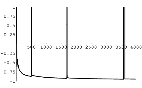
Fig. 2.5 shows the average photon number from Eq. 2.42 together with the rate equation result. We see that the fully quantized theory agrees with one of the rate equation stable solutions except during “jumps” corresponding to transitions between the solutions. The quantum theory essentially “chooses” one of the rate equation solutions.
During the transitions, which become increasingly narrow as is increased, the photon number distribution has two peaks corresponding to the two stable solutions.
It can be shown that the rate equation solutions correspond to within of a local maxima of the distributions from the quantum theory. Suppose a local maximum in exists at ; this means that and the quantity inside the product of Eq. 2.42 passes through 1 between and :
| (2.47) |
Setting
| (2.48) |
gives the original rate equation Eq. 2.25.
2.4 Modification for realistic parameters
We describe modifications to the rate equation and quantum theory in order to accomodate the atomic velocity distribution, nonuniform atom-cavity coupling, atom-cavity detuning, and imperfect pumping.
2.4.1 Averaging of gain function
The framework for all these modifications is the same: we calculate the effect of the relevant broadening on the “gain function” which for an ideal (monovelocity etc.) microlaser is given by
| (2.49) |
For example, the effect of a velocity distribution is the average
| (2.50) |
The steady-state photon statistics are then given by
| (2.51) |
Note that we essentially replace a process in which different atoms experience different interactions, with a process in which all atoms experience the same averaged interaction. This may seem implausible until we realize that the end result 2.51 represents an average itself. Our averaging procedure follows from the assumption that the random variables associated with the velocity, etc. are independent (cf. [21]).
The following expression is used to give the average of the gain function over velocity distribution, coupling variation, and detuning:
| (2.52) |
where and is the gain function including detuning. It might be expected that is given by the well-known solution involving the generalized Rabi frequency
| (2.53) |
However, this expression is only valid for constant fields. In general must be calculated numerically and its form will depend on the shape of the coupling profile , not just its area. The function is found by integrating the Bloch equations ( Eqns. 2.15 and 2.16) for a initially excited atom in a field with detuning and Rabi frequency during a simulated transit through the cavity. Integration of for every calculation would be very time-consuming; therefore we tabulate this function on a grid and construct an interpolating function to be called on by our theory calculations.
2.4.2 Imperfect inversion
The adiabatic pumping process described in Chapter 4 is not perfect: for the data shown in the Chapter 5, the excited state probability was about 80%, measured by a fluorescence experiment. This includes a small contribution from atomic decay during the pump process and the transit time between the pump field and cavity mode.
Let and be the upper and lower state probabilities, respectively. We claim that for very large the effect of nonzero is simply to reduce the effective number of atoms to
| (2.54) |
assuming . That is, instead of the number of atoms we may speak of the inversion. This idea is a familiar one in laser physics.
To support this claim we note that atoms initially in the ground state have a probability of removing (absorbing) a photon from the field of
| (2.55) |
Intuitively it is clear that the case would produce essentially zero photons, since the initially lower state atoms absorb photons in the same manner as the upper state atoms emit them.
In the rate equation picture, the net emission rate per atom is then modified to
| (2.56) |
with corrections on the order of . Corrections may affect the initial threshold region somewhat but for most of the range of interest in our experiments, is very large.
Realistic rate equation and quantum theory
Fig. 2.8 gives the equivalent of Fig. 2.5 after realistic effects, appropriate to the data presented in Chapter 5 have been included.


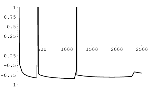
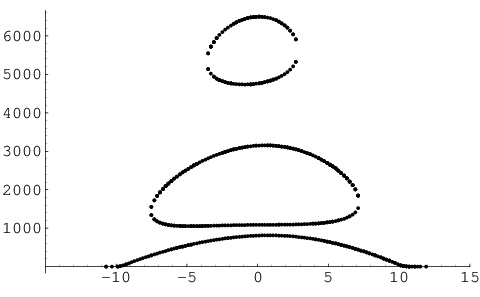
The average photon number can also be plotted as a function of detuning. (Fig. 2.11).
Detuning,

2.5 Fokker-Planck analysis
In [21] a Fokker-Planck equation for the cavity photon number distribution is derived:
| (2.57) |
where for zero thermal photon number
| (2.58) |
| (2.59) |
and is the injection rate. To generalize to our averaged case we replace the terms with from 2.52. (The replacement of by is insignificant on the photon number scale we will consider.) Equation 2.57 was shown to reproduce the average photon number and photon statistics of micromaser theory as long as (i) the pump parameter and (ii) . Both of these conditions are easily met in our case.
We now rescale time to the cavity lifetime and photon number to expectation photon number: , . Then Eq. 2.57 becomes
| (2.60) |
with
| (2.61) |
| (2.62) |
noting that .
The stationary solution to the Fokker-Planck equation is then
| (2.63) |
where is a normalization constant. For large the photon number distribution will accumulate in the global maximum of the exponent of Eq. 2.63, or equivalently the global minimum of an effective potential defined by
| (2.64) |
The local minima of are the zeros of , which are the solutions of
| (2.65) |
which is equivalent to the rate equation derived in 2.25.
We now have an intuitive picture for the transitions between stable points: they occur as the global minimum of the effective potential changes from one point to another. This is a variation on the Landau theory of phase transitions, with as the order parameter. Note that as the transitions become infinitely sharp in a similar manner to the sharpness of phase transitions for a large number of particles.
We note that the initial threshold is of second-order: as the injection rate is increased there is a continuous increase of the global minimum in the effective potential from .
2.5.1 Metastability and hysteresis
In general the microlaser does not automatically find the global minimum but must fluctuate to it from out of a local minimum. Therefore hysteresis is expected if parameters are varied faster than the transition rate between metastable and stable states.
To give an example, let us consider the rate equation solutions as detuning is varied. As shown in Fig. 2.11 the first branch appears as an inverted parabola-type shape centered around zero detuning (relative to resonance of most probable velocity atoms); higher branches first appear as closed curves, and with increased atom number, join with the first branch solution. (See Fig. 2.12). Suppose that metastable lifetimes are very long and spontaneous transitions do not occur. Then as detuning is modulated we would expect a consistent hysteresis pattern following the arrows in Fig. 2.12). These transitions occur when parameters change so that a local minimum in the potential disappears entirely, and the system is forced to the next potential minimum it encounters (not necessarily the global minimum).
Similar features would be encountered for photon number as a function of atom number.

Detuning, , for experimental parameters.
2.5.2 Transition rates
The tunneling rate from a metastable solution to a global minimum is estimated via the Kramers analysis [21] to be, in units of cavity linewidth,
| (2.66) |
where is the metastable local minima point and is the local maximum over which the system must tunnel to reach a global minimum (or possibly another, lower energy, metastable local minimum). (Fig. 2.13)

Chapter 3 Numerical simulations of many-atom microlaser
We present results from quantum trajectory simulations of a microlaser/micromaser device in which more than one atom at a time may be present and atom transit times are not required to be much smaller than the cavity decay time. For parameters in which the system is well removed from the influence of trap states the average photon number is in good agreement with an appropriately scaled single-atom, weak-decay micromaser theory. The photon number variance, however, shows an increase proportional to for parameters in which the weak-decay theory predicts sub-Poisson statistics.. This result is similar to that found by Elk in the case of regular atomic injection [24]. By considering the case we show that this broadening of the photon number distribution is not a many-atom or correlation effect, but is due to cavity decay during the atom’s transit through the cavity.
3.1 Introduction
The microlaser and micromaser differ from conventional lasers and masers not only in that they use single atoms as the gain medium, but in the controlled nature of the atom-cavity interaction. Uniformity of the coupling strength between atom and cavity [10] and interaction time of the atom through the cavity, in addition to the long lifetime of the atom upper level state compared to the transit time, create an unusual situation in which different atoms undergo nearly the same interaction with the cavity. That is, interaction is almost independent of decay and other random effects. This is in contrast to descriptions of a conventional laser [20] in which ensemble averages are performed to account for the lifetimes of the excited atoms, inhomogeneous effects, etc.
It is natural to ask which properties of the microlaser/micromaser persist even when the restriction of a single atom is lifted. Dynamics based on single-atom quantum Rabi oscillations are not necessarily expected to hold; in addition, correlation effects may cause unknown differences from single-atom theory.
A related problem is to determine the effect of abandoning an assumption made in analytical treatments of the microlaser/micromaser [21] that the cavity decay time is much longer than the interaction time, i.e. where is the cavity linewidth. In this paper we will call this the condition of weak decay.
The present study was motivated by the realization that with the current experimental parameters, more than one atom at a time must be present for laser oscillation to occur. In going from the standing wave to the tilted atomic beam, uniform-coupling, traveling-wave interaction [10] the coupling strength is decreased by a factor of 2 relative to the peak standing-wave value. (This factor of 2 was incorrectly reported as a factor of in [10].) The threshold number of atoms is given by [21]:
This is to be compared with for the original (standing wave) microlaser experiment [8] if is taken at an antinode. Therefore the study of multiple atom effects is necessary for understanding the microlaser with traveling-wave interaction.
Effects relating to finite are also of interest in the microlaser, since with present parameters [10] we have .
3.2 Previous approaches
The effect of 2-atom events was studied in [73] in the context of micromaser trap states. It was shown that collective events destroy trap state resonances with great efficiency.
More general treatments of multi-atom behavior have involved strong simplifications to the atom injection scheme.
D’Ariano studied a micromaser system pumped by clusters of up to atoms which all enter and leave the cavity at the same time [25]. It was shown that for the system behaves similarly to the one-atom maser, and for the system exhibits multiple thresholds.
Elk [24] considered an injection scheme in which atom arrivals are equally spaced in time. Results for small and showed a nearly constant average photon number but a linear increase in photon number distribution width with . However, it is difficult to determine whether the results are related to regular injection of atoms, which in general causes a reduction of noise (i.e. smaller ). We note that the results in the case do not agree with single-atom micromaser theory [21].
In this paper we study the case of realistic, Poisson atomic injection, and interpret the results based on finite transit-time rather than many-atom effects.
3.3 Quantum trajectory analysis
To simulate the microlaser with random (Poisson) injection of atoms, we used a quantum trajectory algorithm [32],[33]. This technique was previously used to analyze the threshold-like transition, and the possibility of many-atom effects, in the original standing-wave microlaser in [30]. This paper contains for a detailed description of the extended quantum trajectory technique also employed in the present study.
Due to limitations of computer memory and processing time, for each simulation run it was necessary to set a maximum value for the number of atoms that could be present in the cavity at a given time. In each case was adjusted such that the “overflow” probability was 1% or less, ensuring that the statistics are very close to Poissonian.
In single-atom micromaser theory [21], the behavior of the system is determined by three parameters: (i) the expected photon number where is the atom injection rate; (ii) the pump parameter where is the atom-field coupling constant; and (iii) the thermal photon number .
It is then shown that, with the assumptions of single-atom events and (weak decay), [21] the steady-state photon number distribution in the cavity is given by
| (3.1) |
where is determined by normalization. In this paper Eq. 3.1 will be referred to as the result from micromaser theory, although it is also applicable to the microlaser.
In this study we set thermal photon number
We performed runs of 10,000 – 100,000 atom injections, for varying values of , and number of intracavity atoms . We scaled and as necessary to obtain the correct values for and as was varied. At the beginning of each run, at least 2,000 atom injections were neglected in order to allow the system to reach steady state before data collection began.
Most simulations were performed with . This value was chosen for several reasons. First, a relatively low photon number allows larger numbers of atoms to be considered. Second, effects that scale as are more apparent for smaller . Finally, we observed that simulations reached their steady-state distributions much more rapidly for lower .
For simplicity, and to allow comparison with analytic theory, we regard and to be perfectly well-defined (i.e. uniform coupling and monovelocity atoms). Our QTS program has also allowed us to simulate the effects of various types of variation and broadening in a realistic system. Results of these investigations will be reported elsewhere.
The simulation was written in C (see Appendix) and all calculations were performed on a 400 MHz Pentium II workstation running Linux. The calculations presented here required roughly 2000 hours of CPU time in total.
3.4 Results
3.4.1 Single atom limit; Trap states

Fig. 3.1 shows the average photon number as a function of , for . Note the deep depressions due to trap states resonances in which atoms perform integral numbers of Rabi oscillations.
With the QTS results for average photon number show significantly smaller modulation due to trap states than the result of Eq. 3.1 although the probability of the cavity containing 2 or more atoms at any given time is . It is only with that QTS results give good agreement with micromaser theory. This illustrates the sensitivity of the trap state resonances to 2-atom events as described in [73].
The photon number distributions in the low- limit were verified to be in excellent agreement with Eq. 3.1, further confirming that the simulation was working properly.
3.4.2 Broadening of photon number distribution
Figs. 3.2 and 3.3 show values of average photon number and Mandel parameter as a function of for a range of atom numbers , with . Note that for larger values of , is large and may be difficult to interpret due to the presence of 2 or more peaks in the photon number distribution.


For , before the trap state resonances occur, the results for average photon number remain remarkably close to the prediction of micromaser theory. The values for , however, show a significant increase with in the range . This interval corresponds to the region in which according to micromaser theory the system displays sub-Poisson statistics ().
Similar increases in are observed in a small interval near , between two trap states. Simulations with 30 and , in which trap state resonances are more narrow, showed similar behavior over wider intervals between trap states.

The parameter was calculated as a function of , with , for , , , . The increase of is seen to be linear with ; for we find (Fig.3.4) that all points may be approximately described by
| (3.2) |
where is the value of the Mandel parameter from micromaser theory and .

Fig. 3.5 shows calculated via a least-squares fit with and . Error bars indicate the degree of linearity. It is seen that exhibits oscillation with and is positive for where the single-atom, weak-decay theory predicts sub-Poisson statistics ().
3.4.3 Many-atom vs. finite transit time effects
An increase of variance proportional to was previously found by Elk, who interpreted it as being due to many-atom interactions [24].
We note, however, that is equal to simply , a parameter describing cavity decay during the transit time, and is not directly related to the number of atoms. The extra variance observed in this study and by Elk can therefore be seen as a consequence not of multiple atoms, but of cavity decay during an atom’s transit time. For example, we may have but virtually no extra variance if . More importantly, there are examples in which but excess variance still occurs. Fig. 3.6 shows as a function of for , . A linear increase in variance is seen even for .

3.5 Predictions for experiment
To apply our quantum trajectory results to our microlaser system, we make a seemingly precarious assumption that simulations for atoms represent the behavior for up to . If true then the predictions for the experiment are as follows.
No significant deviation from the single-atom theory was found for the few-atoms microlaser; therefore we would expect the cavity photon number to follow the prediction of the microlaser with realistic parameters described in Sec. 2.4, as plotted in Fig. 2.8.
For the photon statistics, we have in the microlaser , and therefore the perturbation to photon statistics is fairly small; it would not differ strongly from that given in Fig. 2.9.
An upper-bound prediction for the parameter is given in Fig. 3.7.

3.6 Discussion
Our calculations have clarified the distinction between many-atom effects and effects due to cavity decay during transit-time. Many-atom events destroy the trap state resonances and therefore have strong effects for parameters for which these resonances are prominent. Away from these resonances, the system shows remarkable agreement with single-atom micromaser theory. However, for values of for which micromaser theory predicts sub-Poisson statistics, cavity decay during transit time cause an increase in variance relative to micromaser theory, by an amount proportional to .
Lack of collective effects away from trap states may be a consequence of the noncorrelated Rabi phases of atoms which have entered the cavity at different times. Increase of variance represents an absolute decrease in the negative differential gain in the atom-cavity system. Future work will include development of models to explain the observed effects quantitatively.
Chapter 4 Apparatus and methods of microlaser experiment
In this chapter we describe the components of the microlaser and techniques used in its study. In particular we describe how a well-defined interaction between atoms and cavity can be achieved.
4.1 Two-level atom
4.1.1 Barium energy levels

Figure 4.1 shows the levels of relevant to the microlaser experiment. The microlaser uses the transition of wavelength nm and linewidth approximately 50 kHz. The excited state decays to the ground state and two metastable D states with a branching ratio of 0.43:0.41:0.16. We use this intercombination line due to its relatively long lifetime .
The most frequently studied transition in is at 553 nm. It has a linewidth of about 19 MHz. The fluorescence spectrum of a naturally occuring barium sample is shown, with isotope shifts, in Fig. 4.2.
The 553 nm transition was used to measure atomic density in the cavity, determine pump beam efficiency, and measure the atomic velocity distribution.

Natural occuring barium, of which 71.7% is , is relatively inexpensive and readily available. We purchased the metal in rod form, packed in argon, from Alfa Aesar.
4.2 Optical resonator
The microlaser cavity mirrors consist of superpolished fused silica substrates coated with a multilayer, ion-sputtered dielectric coating. The substrates and coatings were purchased from Research Electro-Optics (Boulder, Colorado). The coating consists of 45 alternating layers of and .
4.2.1 Characteristics
The microlaser cavity consists of two mirrors in a symmetrical, near-planar Fabry-Perot configuration. The mirror separation, measured via transverse mode spacing, is 1.1 mm. The radius of curvature of the coated surfaces is 10 cm.
The mirrors have an overall diameter of 7?mm and length of ? mm. The actual reflective surfaces are 45-degree beveled to a diameter of 3 mm in order to facilitate alignment of the tilted atomic beam and cleaning of the coated surfaces.
The mirrors are glued into stainless steel holders (Fig. 4.3) designed to hold the mirrors without birefringence-inducing stress. The cavity is aligned outside the chamber, then the holders are glued on the inside of a cylindrical piezo transducer (PZT) used to modulate the cavity mirror spacing.


The microlaser experiment is performed with the fundamental (TEM00) mode of the cavity (it is also possible to use higher-order transverse modes). The mode waist is given by
| (4.1) |
where is the mirror radius of curvature, is the cavity spacing, and is the wavelength.

The cavity mode volume is given by
| (4.2) |
and the peak atom-cavity coupling for the standing-wave case is
| (4.3) |
The atom-cavity interaction time for a particular atom is defined as
| (4.4) |
where is the atom’s velocity. The factor accounts for the Gaussian shape of the cavity mode: the integral of with time for a moving atom is the same as an atom of the same velocity traversing a “top hat” mode of constant coupling for time :
| (4.5) |
The cavity spacing was determined via measurement of the transverse mode spacing. In a near-planar cavity,
| (4.6) |
where higher-order corrections can be shown to be for our cavity [82, ch. 19].
We determined by measuring the difference in PZT voltages between the fundamental and first transverse mode resonances. The scan was calibrated by measuring the PZT voltage shift between two sidebands of the 24.67 MHz FM modulation used for laser frequency locking (see Sec. X). We find the PZT scan calibration is 171.6 MHz/V and verified that it does not vary measurably over the PZT voltage range in question. The transverse mode spacing was measured to be
| (4.7) |
giving a cavity length
| (4.8) |

4.2.2 Cavity PZT
The PZT controlling the cavity separation is a tube (Vernitron PZT-5A) of height 0.75” and inner diameter 0.75”, and wall thickness 0.125”. Four holes are drilled in the cylinder wall to allow passage of the atom and pump beams.
Isolation mechanisms are used to isolate the cavity from vibrations. Viton o-rings hold the PZT inside a heavy brass housing (Fig. 4.3). The housing is placed in a supporting structure by fittings made of teflon (Fig. 4.5); the support in turn is secured inside the vacuum chamber with teflon screws.
4.2.3 Finesse measurement by ringdown technique

The finesse of a Fabry-Perot cavity is defined as the ratio of free spectral range (FSR) to the FWHM of a cavity transmission peak, or equivalently.
| (4.9) |
where is the geometric average of the intensity reflectivity of the two mirrors, i.e. and we assume very close to unity.
To measure finesse we scan the cavity PZT through resonance with a probe laser beam. The cavity decay time is measured by fitting a curve to the exponential decay of the cavity field (Fig. 4.8). The signal shows a sinusoidal modulation due to interference between the probe beam and the Doppler-shifted cavity field. This is described further in Ref. [36].
4.2.4 Absorption measurement via thermally-induced optical bistability
The finesse is given by , with the mirror reflectivity and the total loss, equal to the sum of three loss parameters, the absorption , scatter and transmission . R, hence the total loss, can be measured by cavity ringdown [36]. However, determining how the loss is distributed among , and is difficult. In particular, few techniques exist for measuring very small absorption coefficients. Methods such as photothermal deflection [37] are capable of measuring down to 1 ppm.

Recently we have developed a new technique to measure at the sub-ppm level [38, 39]. This technique relies on the intense circulating field created when a resonant probe beam is incident on a high finesse cavity. Any absorption of the intense internal field causes heating in the coating layers, and the subsequent thermal expansion of the mirror substrate reduces the mirror separation distance and leads to a thermally-induced optical bistability of the empty resonator. This optical bistability causes distortion in the measured cavity lineshape, as observed by slowly scanning the cavity length. The lineshape exhibits an extended resonance with a slow rise and rapid drop (Fig. 4), the duration of the resonance being directly related to the absorption coefficient [38].
We have characterized all three parameters and established that ppm and ppm, thus establishing that scattering is the predominant loss mechanism in our supercavity mirrors [39].
4.2.5 Uniform coupling by traveling-wave interaction
In the original microlaser experiment, the atom beam is incident normal to the cavity axis and atoms interact with the standing wave of the Fabry-Perot cavity. Since the coupling is proportional to the local field amplitude, which varies as , atoms experience a wide range of coupling strengths.
We eliminated this problem by introducing a small tilt between the atom beam direction and the normal to the cavity axis. Due to the Doppler shift, each atom then experiences not one standing wave but two traveling waves of frequencies . If is sufficiently large, the atom will be resonant with only one traveling wave component at a time. This eliminates the fast spatial variation due to the standing wave. It should be noted that in the traveling-wave configuration the peak coupling constant, , is reduced by a factor of compared to the peak standing-wave value (see Appendix D). (This factor of 2 was incorrectly reported as in [10].)

4.3 Atomic beam
A typical atom beam apparatus consists of a container in which the sample is heated in vacuum to form a vapor; a small nozzle allows vapor atoms to escape. Apertures are placed downstream to collimate the beam.
We have two main requirements for our barium atomic beam: high beam density and narrow velocity distribution in the ground state.
4.3.1 Velocity selection: mechanical, optical, or supersonic
An atomic beam with narrow velocity spread is needed to provide a well-defined atom-cavity interaction time (i.e. uniform transit time), and to ensure that all atoms traversing the pump laser field prior to entering the cavity are excited to a state of complete inversion ( pulse condition).
The “classical” technique of mechanical velocity selection (via e.g. Fizeau wheel) has several serious drawbacks: the beam created is pulsed, not continuous, and the overall efficiency is low.
Two new methods for creating narrow-velocity ground state atom barium beams have been developed in our laboratory.
4.3.2 Atomic velocity selection via optical pumping
We have developed a two-color optical pumping method for selectively preparing atoms in the ground state at a certain velocity, in an effusive beam. The beam is created in a cylindrical, externally heated oven made of Inconel. Continuous-wave lasers are used to pump tbe barium atoms, first into the metastable 1D2 state via the 6s2 1S 6s6p 1P1 cycling transition (=553 nm), and then back to the 6s2 1S0 ground state with velocity selectivity via a tilted laser tuned to the 583 nm 6s5d 1D 5d6p 1P1 transition (Fig. 4.11). When the most probable velocity is selected we obtain with approximately 50% repumping efficiency (Fig. 4.11).


4.3.3 Supersonic oven
Background
Supersonic beam techniques have found many applications in spectroscopy and atom interferometry since their invention in 1951 [78, 79, 80]. In a supersonic beam, adiabatic expansion as the beam exits the oven nozzle causes a dramatic cooling in the frame of the moving atoms or molecules; random thermal energy is converted into directed kinetic energy. In addition, the net flow rate is generally much higher than for an effusive beam. This solves the two problems associated with conventional effusive beams: low intensity and a wide distribution of velocities.
Supersonic barium oven: apparatus
We have developed a supersonic beam oven for barium closely following the design of Ref. [81], which was based on an effusive beam source developed in our laboratory and previously used for the microlaser experiment [8].
The atomic beam oven consists of resistively heated, barium-filled piece of tantalum tubing, in which a small nozzle hole has been drilled. A diagram in shown in Fig. 4.13. The tubing is 6.5” long, 0.5” in diameter, with 0.015” wall thickness. The nozzle diameter varied from 150 to 406 .
Like the atoms strontium and ytterbium used in Ref. [81], barium has two valence electrons and negligible dimer formation.

The oven is created by the following procedure. A length of tubing is measured and cut with a pipe cutter. The bottom 1.125” is pinched flat in a vise between two aluminum blocks. One quarter of a 2 cm diameter barium rod (cut by bandsaw lengthwise) is inserted into the tantalum tube. The typical mass of barium in one oven is 12-16 g. The top 1.5” of the oven is then flattened in a vise, parallel with the bottom of the oven. The oven is mounted in a specially designed holder to position it with flat parts horizontal. It is clamped in a milling machine where a 1/8” end mill removes about 0.007” from the future location of the nozzle. This gives a shorter “channel” for the atom flow and creates a flat surface for drilling the nozzle, which is done in a miniature drill press.
In the experiment, the oven is clamped by two screws at each end between copper electrodes. The upper electrode is connected to a copper tube which extends through an 8” Conflat flange via a 3/4” diameter Ultra-Torr fitting. The bottom electrode is soldered to a 4” diameter copper cold shield tube which both absorbs the oven’s large thermal radiation and conducts current back up to the flange coaxially with the central conductor, to minimize stray magnetic fields from the oven. The upper and bottom electrodes and the cold shield are cooled by water flowing through 1/4” copper tubing which has been soldered to the copper pieces.
A Proteus flowmeter placed on the return path of the oven cooling water is connected to a lamp which provides visual feedback that the water is flowing.
The oven drive current is controlled manually using a variable Variac autotransformer with 208 VAC line input and 0-230 VAC output. The Variac output is connected to a step-down transformer with 1:8 turn ratio, and the resulting output is connected to the center conductor and top oven flange (ground) via 2 pairs of 1” diameter welding cables. The oven voltage and current are monitored by AC voltmeter and a clamp-on ammeter. The voltage varies from 0-5VAC and current 0-1000 A rms?. The resistance of the entire circuit varies from approximately 4 m to 6 m depending on oven temperature.
Supersonic barium oven: results
As oven power is increased, the beam density increases and the beam undergoes a transition from Maxwell-Boltzmann (thermal) velocity distribution to supersonic velocity distribution.
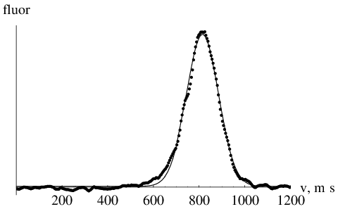
We measured the atomic density and velocity distribution via 553 nm fluorescence. To measure density, the 553 nm beam was aligned to overlap the 791 nm probe beam along the cavity axis and the fluorescence was detected by CCD (see section 4.6). Velocity distribution was measured by aligning a focused 553 nm beam in the cavity in a direction opposite to atom beam direction, and detecting the Doppler-dependent fluorescence via a photon counting APD (EG&G C30902TE) previously aligned with the cavity transmission. A 500 diameter pinhole located in front of the APD and mounted on an XY translation stage blocks scattered light from the ground glass beveled edges of the cavity mirrors.
Figure 4.14 shows the velocity distribution for the supersonic beam used in the experiments. This oven had a nozzle size of 406 and was driven by about an rms current of about 600 amperes.
The degree of velocity compression can be characterized by the ratio between FWHM of the measured velocity distribution and most probable velocity .
The measured velocity distribution is equal to the actual velocity distribution convoluted with a lineshape function accounting for atom linewidth and isotope shifts. Laser power broadening effects can be minimized by using a probe laser beam intensity well below saturation.
Although the supersonic expansion results in a higher velocity and thus smaller interaction time (roughly by a factor of 2), there are several advantages of the supersonic oven. First, and most importantly, velocity narrowing gives higher densities than velocity selection because non-selected atoms are lost in the latter. In addition, the supersonic beam gives far higher densities than even a non-selected thermal beam, due to the higher oven temperatures. Experiments with the supersonic beam are simpler because the additional lasers and locking systems are not needed. Due to these advantages, all of the microlaser experiments in this thesis were done with the supersonic beam.
4.3.4 Final aperture
The small dimensions of the microlaser cavity mode place strong constraints on the size and location of the atomic beam. It must be small and closely centered on the mode if reasonably uniform coupling is to be obtained.
Variation due to the Gaussian shape of the cavity mode can be made relatively small by limiting the dimensions of the atomic beam inside the cavity. For an atomic beam of height centered in the mode, the ratio of minimum to maximum coupling is
| (4.10) |
This value is plotted in Figure 4.16. For a beam size of 25 we have


In order to create a small beam in the cavity we collimated the atomic beam with a 24.5 diameter aperture placed approximately 3 mm from the cavity axis. The distance between aperture and cavity is important because a larger distance increases the broadening of the atom beam due to the finite solid angle of the atom beam source (i.e. oven nozzle). The aperture was mounted onto a thin, hollow, tapered “pencil” which fit into the hole drilled into the PZT to allow passage of the atomic beam. The pencil is attached to the center of a 1/2” stainless-steel compact mirror mount which allows the orientation of the pencil to be modified precisely. The mirror mount was mounted on a miniature motorized rotation stage (National Aperture MM–3M–R). A stepper driver (National Aperture MC-II) located outside the chamber is connected to the rotation stage by a 10-pin electrical feedthrough. The mirror mount adjustment screws were tweaked so that center of rotation is located at the center of the aperture. Finally, the rotation stage and aperture assembly were connected to an XY miniature translation stage (National Aperture ST1XY) which could be manipulated from outside the chamber through two inch Ultra-Torr feedthroughs. The feedthroughs couple to the stage via flexible couplings.
The pencil has a tapering design in order to be small enough at the tip to approach the cavity closely, and yet large enough to accomodate a range of atomic beam angles and avoid clipping the beam. The pencil was made from several pieces of brass telescoping square tubing, glued together with Varian Torr-Seal vacuum epoxy. The aperture (12.7 thick stainless steel, from National Aperture) was attached to the pencil tip with Torr-Seal.


To center the atomic beam on the cavity mode axis, we monitored the microlaser emission power as a function of atom beam vertical position (measured by imaging the aperture with the imaging system described in Sec. 4.6). By this method we are able to find the center of the mode to a few . A typical result is shown in Fig. 4.19. Repeated measurements are taken as the aperture position is varied; low points are due to fluctuations in chamber pressure when the feedthrough is manipulated. Aperture position is measured by the CCD pixel number corresponding to the maximum intensity in an image of the oven blackbody radiation passing through the aperture.

4.3.5 Atom density modulator
The density, peak velocity, and velocity compression of a supersonic beam are all functions of the oven current (i.e. temperature) and the amount of barium remaining in the oven. During our experiment, we would like to vary the density only. Therefore the oven current alone cannot be used to modulate density in the cavity, as it was for the original microlaser experiment [8] or some recent experiments [84]

We have introduced a variable beam density modulator which intercepts the atomic beam between the oven and cavity and prevents some or all of the atoms from entering the cavity. The modulator consists of a piece of sheet aluminum attached to a motorized linear feedthrough (Huntington L-2251-2) mounted at the 6-way cross between oven and cavity. This is shown in Fig. 4.20. The aluminum piece was initially cut in a wedge shape in order to give a longer modulation range as it is moved vertically. This was later found to be unnecessary as sufficiently high resolution was obtained with a flat piece of aluminum. The modulator is located 21 cm from the oven; the cavity is 42 cm from the oven.
The linear feedthrough has a lead of ” per revolution. The stepper motor turns one revolution per 200 steps, giving a linear resolution of per step. Higher resolution is possible via microstepping. Full linear travel is 2”.
The stepper motor is controlled by an Intelligent Motions Systems Panther LI2 (aka Huntington MLC-11) Driver. This driver was found to create a great deal of electromagnetic interference in the laboratory, which was reduced using a set of opto-isolators and line filters. The driver is controlled by a PC via a standard RS232 serial connection. The driver is equipped with 3 logic-level auxiliary outputs which were used to control other experimental parameters (described in section 4.11.1).

The cavity fluorescence signal as a function of modulator position is shown in Fig. 4.21
4.4 Laser systems, locking, and stabilization
4.4.1 Laser equipment
Two tunable lasers were used in the microlaser experiments. To provide the 791nm microlaser pump beam and cavity probe, we used a Coherent 899-21 Titanium-Sapphire ring laser pumped by an Innova 310 argon ion laser operating at 8W in multiline visible mode.
A Coherent 699-21 dye laser tuned to the 553 nm transition was used to monitor atomic density in the cavity and measure the atomic velocity distribution. The dye used in this laser was Rhodamine 110. The laser was pumped by an 8W multiline visible beam from a Coherent Innova 200 Argon ion laser.
4.4.2 Frequency stabilization of 791 nm beam by Doppler-free FM spectroscopy
Frequency locking of the Ti:Sapphire laser to the transition was done by a standard FM modulation technique. This locking system is described in detail in [83].
An evacuated stainless-steel cylindrical cell containing about 2g barium is heated to C by external heating elements to produce a barium vapor. Pump and probe laser beams pass through the cell from opposite directions, through two glass windows. The probe beam first passes through an electro-optic phase modulator (EOM) driven at 24.6 MHz. After passing through the cell the probe beam is incident on a photodiode (Thorlabs DET110). The signal is amplified and demodulated via mixing with the 24.6 MHz local oscillator signal in a double-balanced mixer (Minicircuits). The relative phase of the two inputs to the mixer is adjusted by varying the modulation frequency and the lengths of BNC cables to produce a maximum dispersion signal, shown in 4.23. The dispersion signal is amplified and shifted to remove any DC offset from the mixer. It has a zero crossing at the peak of the Lamb dip (atom resonance). To lock the laser to the zero crossing, the dispersion signal is fed back to to Ti:Sapphire laser as an error signal in place of the signal from the reference cavity. The linewidth of the lock is estimated as approximately 300 [83].


4.4.3 Locking of 553 nm beam to atomic beam
The 699-21 dye laser was locked to the transition via a different Lamb dip technique. After reflection through a beamsplitter, a strong 553 nm pump laser beam is incident on a barium cell heated to 490 C. The transmission through the cell is apertured then retroreflected back into the cell, overlapped by the original beam. The reflected beam forms the probe, which is detected by a photodiode (Thorlabs DET110) after the beamsplitter. The resulting absorption signal shows a Lamb dip (Fig. 4.24).

Detuning, GHz

The laser locking system consists of an integrating amplifier and summing amplifier. A local oscillator at about 300 Hz frequency, 100 mV peak to peak amplitude dithers the frequency of the dye laser through the external horizontal input of the laser control box. The photodiode signal and local oscillator are connected to a lock-in amplifier. After adjusting the phase, the output signal is of dispersion type, with zero crossing at the peak of the Lamb dip. This signal is fed to an integrating amplifier, which controls the DC offset of the laser external input. The resulting lock stays within approximately 2 MHz of resonance. This is much smaller than the 19 MHz natural linewidth of the transition and was judged to be adequate.
4.4.4 Intensity and position stabilization
Both the 791nm and 553nm lasers experience some short-term and long-term intensity fluctuations. The dye laser has considerable ( ) noise in the kHz range and the average intensity decreases gradually over hours as the dye decays. The Ti:Sapphire laser has little short-term noise but does have slow intensity fluctuations, most likely due to pump beam wander.
Pump beam wander, thermal effects, daily power peaking, and other effects cause substantial variations in laser beam direction from day to day and within single days. Often these effects are corrected for by aligning a laser beam through two adjustable irises. However, since many aspects of the microlaser experiment require very precise beam positions (micron scale) and angles (milliradian scale), irises do not provide adequate repeatability.

To reduce laser intensity noise and stabilize long-term power, and to stabilize laser positions, we have developed a laser stabilization system. Acousto-optic modulators (AOMs) are used to cancel intensity fluctuations. Coupling through single-mode optical fibers allows very consistent optical alignment of beams with respect to the setup.

The intensity stabilization system uses a photodiode and integrating amplifier to provide feedback through an AOM VIDEO signal. A photodiode connected to a variable-termination, transconductance amplifier monitors the laser power after the single mode fiber as shown in Fig.4.26. The photodiode signal is compared with a target voltage and the difference is passed to an integrating amplifier, the output of which is connected to the AOM VIDEO input (amplitude modulation). The output voltage range is trimmed by potentiometers to correspond to a range from minimum to maximum AOM transmission.
Polarization maintaining (PM) single-mode fibers are used to stabilize the position of the 791 pump beam and the 553nm probe laser beams. We use 1m long Newport SP-V fiber for the 791nm beam and a 5m Newport SP-? fiber for the 553nm beam. A schematic is shown in Fig. 4.26.
4.5 Pump beam
The pump beam is supplied by the FM-locked Ti:Sapphire laser. The problem of how to pump the atoms correctly proved to be more complicated than expected, and led to the rediscovery of a method for inverting atoms by a defocused laser beam.
The pump beam intersection with the atomic beam must be sufficiently small that upper state spontaneous decay does not significantly affect the final degree of inversion. For the same reason, the pump beam spot must be placed close to the cavity mode, but without overlap.
Other critical parameters include the angle between the pump beam and atom beam direction (ideally exactly 90 degrees), total pump power, location of pump focus, uniformity of the pump beam intensity over the width of the atomic beam, and laser frequency jitter about the atom resonance.
4.5.1 Optical setup
As described in Sec.X the pump beam is coupled through a single-mode polarization-maintaining (PM) fiber for intensity and position stabilization. The emerging beam is collimated by an aspheric lens and passes through a beam steering apparatus to raise the beam height above the vacuum chamber.
The pump beam steering apparatus is illustrated in Fig. 4.28. It consists of mirrors and a lens mounted on translation stages such that one stage controls the pump beam focus and one controls the pump beam position (in the z direction), nearly independently.
The lens is a single element, BK7 plano-cylindrical lens with focal length 400? mm. Tests using the CCD camera as a beam analyzer showed that a nearly diffraction-limited spot size of 35 could be achieved at the focus.
The pump beam is reflected down into the cavity by an 2” diameter, 45-degree-angled dichroic beamsplitter which has reflectivity approximately 90% at 791 nm and 10% at 553 nm. A dichroic beamsplitter is used instead of a mirror in order to allow imaging of 553 nm fluorescence from above the beam splitter. In addition, the weak 791 nm transmitted beam can be used to analyze the focus and beam quality of the pump.

The window on the top of the chamber is an anti-reflection coated glass disc held in place by a custom metal flange and Viton O-rings.
A coil-generated magnetic field of approximately 50 gauss parallel to the direction of pump polarization (perpendicular to the cavity axis) splits the -states by about 50 and ensures that only transitions between sublevels and occur.
4.5.2 Pump beam parameters
Here we describe the optimization of the pump beam parameters in more detail.
Pump beam focus
The pump focusing lens is placed approximately one focal length away from the cavity. To find the focus more precisely, we overlap the 791 nm pump with a resonant 553 nm probe beam. With the imaging system (Sec. 4.6) in the top viewing configuration, we take pictures of the fluorescence of atoms in the probe field. By measuring the width of the fluorescence spot as a function of the pump focus translation stage micrometer, we can find the focus of the 553 nm beam. However, this is in general displaced from the 791 nm focus due to lens dispersion and different laser beam divergences of the beam before entering the pump beam setup. To address this problem we used the CCD camera, without lenses, as a laser beam analyzer for the 791 nm and 553 nm beams transmitted by the dichroic beamsplitter. The CCD position was positioned the same distance from the beamsplitter as the cavity is from the beamsplitter. The camera was moved by a translation stage to locate the positions of the 553 nm and 791 nm beam foci. This gave the displacements of the two beam waists, typically about 1 cm apart. The pump focus was then adjusted by this amount to place the 791 nm focus as close as possible to the atoms in the cavity.
This procedure was not perfect: as described in Sec. 4.5.5, significant pump defocus was found to occur.
Pump position
Pump position can be monitored by a number of methods involving the 553 nm transition and the imaging system. However, the most effective methods is to monitor the microlaser output power as a function of pump position. When the pump is placed downstream of the cavity mode, no emission is seen. For pump beam overlapping the mode, a signal with unequal traveling-wave peak heights is usually observed. The reason for the unequal traveling-wave peaks is not clear. For pump beam upstream of the cavity mode, a signal is observed that is nearly flat, with a small slope corresponding to increasing atomic decay with pump-mode distance.
In our experiments we aim for about 100 separation between the pump field and cavity mode. At this distance, which is admittedly somewhat arbitrary, atom decay between pump and mode is quite small,
Pump angle
To minimize Doppler broadening it is important for the pump beam to be as close as possible to perpendicular to the atomic beam direction. Two methods for ensuring this condition were explored. First, we overlapped a 553 nm probe beam over the 791 nm pump as closely as possible, and blocked the 791 nm beam. Then we measured the linewidth of the 791 nm fluorescence as the dye laser was scanned in frequency, and repeated this process as the angle between laser and atom beam was varied. The linewidth increased linearly with any angular deviation from a right angle. This technique was very time-consuming and gave a pump beam perpendicular to the atom beam only to the accuracy that the 791 nm and 553 nm beams were parallel in the cavity. The second technique was to monitor the microlaser output for a constant atom density a few times over threshold, while the frequency of the 791 nm pump laser was varied over a 50 range via the external input of the Ti:Sapphire laser. In this manner, it could be determined if the microlaser power was maximized for positive or negative detunings relative to the atom frequency (i.e. the atoms experienced a blueshifted or redshifted pump field). The pump angle was adjusted until the the microlaser power was maximum with the laser on exact resonance.
4.5.3 Shelving experiment
In order to test the efficiency of the pump process, we perform a “shelving” experiment as follows.
A 553 nm probe beam is aligned with the 791 nm probe which had been matched with the mode of the cavity. Therefore the 553 nm probe field is close to centered on the cavity mode (the beam size may be different, but it will be close to the focus since the 553 nm probe passes through the same achromatic lens). Using the CCD camera, we measure the fluorescence from the atoms in the cavity with and without the pump beam. Since the fluorescence is a measure of the ground state population, the ratio between the fluorescence intensities with and without the pump beam is equal to the average upper state population. If the pump beam were perfectly efficient, no fluorescence at 553 nm would be seen, because all atoms are in the upper state of the transition.
Shelving ratios as low as 10% (i.e. 90% of atoms in the upper state) have been measured.
4.5.4 Pump power dependence of inversion
When the first shelving data was collected, a puzzle presented itself. Atoms interact with the pump beam for a certain time dependiing on their velocity ,
| (4.11) |
where is the waist of the pump beam, assumed to be Gaussian. The excited-state probability for a given atom after leaving the pump beam is expected to be
| (4.12) |
Averaging over atom velocity distribution gives
| (4.13) |
We expect to observe an oscillatory excited state probability damped by the velocity distributions. In the limit of strong field the excited state population should be .

Pump power,
Oscillations as a function of pump power were initially not observed. Instead, we observed the dependence drawn in Fig. 4.29. The excited state population increases monotonically to approximately 80% and does not approach 1/2.
4.5.5 Adiabatic inversion by defocused pump beam
The unusual behavior was explained by the following effect. Suppose there is some distance between the atoms and the focus (minimum waist) of the pump beam – for example, the beam comes to a focus before reaching the atoms. Then the atoms pass through a laser beam which is diverging in the direction of their propagation. As a result, the angle between atom velocity and the wave vector of the pump field varies approximately linearly with position, causing a Doppler-induced frequency chirp through resonance. This leads to an adiabatic inversion process as the atom’s Bloch vector precesses about a relatively slowly varying “torque” which tends to align the atomic Bloch vectors with the inversion axis. A quantitative analysis follows.
Without loss of generality we restrict our attention to the plane containing both the atomic beam and Gaussian beam axis. The phase function of a Gaussian beam depicted in Fig. 4.30 is (see e.g. [85])
| (4.14) |
where is the wave vector, is the Rayleigh range and the wavefront radius of curvature
| (4.15) |

The angle between the Gaussian beam axis and the normal to the phase front can be found via where is the slope of the wavefront (i.e. line of constant ):
| (4.16) |
The sign of the angle is chosen to be positive when the x component of the vector normal to the phase front is opposite the direction of the atom velocity. For simplicity, we consider only the case of atomic velocity perpendicular to Gaussian beam axis.
The equation for simplifies assuming and , both valid easily in our case:
| (4.17) |
The Gaussian waist of the beam as a function of is given by
| (4.18) |
An atom traversing the pump beam at vertical position experiences, as a function of position, the following Doppler shift:
| (4.19) |
The excited state may decay back to the ground state or to a metastable D state. The decay rate to the ground state is and to the metastable state is . The optical Bloch equations describing the pumping process including loss are
| (4.20) |
| (4.21) |
| (4.22) |
| (4.23) |
| (4.24) |
where , , and are excited state, ground state, and metastable state probabilities;
| (4.25) |
| (4.26) |
and is the atom-laser detuning
| (4.27) |
where and are laser frequency and atom resonance frequency. The on-resonant Rabi frequency is given by
| (4.28) |
where and are the Rabi frequency and on-axis laser intensity and is the saturation intensity
| (4.29) |
Fig. 4.31 shows the results of numerical integration of the Bloch equations for different displacements . For the Rabi oscillations are almost completely absent, and inversion occurs almost independently of pump intensity for .

If adiabatic inversion is responsible for the pump power dependence, we should be able to observe Rabi oscillations by focusing the pump beam closer to the atoms (i.e. decrease ). The results are shown in Fig. 4.32. Note that peaks and valleys of the oscillations occur at integer values of . The curve is not asymptotic to for large pump fields; due to uncertainties in the experiment this data may reflect a intermediate state between pure Rabi oscillation and adiabatic inversion.

A quantitative comparison between experiment and theory will be performed in a future study. It has come to our attention that adiabatic following due to a diverging laser beam was previously observed in [86] and [87]. These experiments involve atoms with more complex level structures than the present one.
4.6 Imaging system
A cavity imaging microscope was developed to perform several functions, described below and in following sections.
4.6.1 Setup
The optical design of the imaging system is shown in Fig. 4.33. It can be thought of as a relay lens system combined with a CCD microscope. A 2:1 lens system consisting of two 1” achromatic doublets creates a real image of the cavity. A microscope objective relays the image to a CCD camera. The CCD is positioned at the field focus plane of the objective. The use of microscope objectives gives well-corrected imaging and allows the magnification of the system to be varied easily without realignment. In our experiments we use the 5x objective for the side imaging and 10x for the top imaging (see below for descriptions of the two imaging configurations); the 10x and 20x objectives can also be used in the side imaging configuration when the position of the final collimation aperture needs to be determined precisely.


The achromatic lenses are translatable in 3 directions by translation stages for centering and focusing of the image. The optics, translators, and camera are mounted on an aluminum plate which is fixed to a laboratory jack.
For the side imaging configuration, a 1 inch diameter interference filter (Oriel 53890, nm) is placed between the two achromats to block transmission of the oven’s blackbody radiation. For the top imaging configuration, a color glass filter is used to eliminate pump beam reflection and scatter into the imaging system. This filter has transmission % at 553 nm and 0.1% at 791 nm.
Background light is blocked by a plastic C-mount coupled tube connecting the CCD camera and objective lens, and a sliding cardboard tube covering the optical path between the objective and relay lens.
The CCD used is a Roper Scientific / Photometrics Sensys 400. This camera uses a thermoelectrically cooled, 1/2-inch format, 768 512 pixel Kodak KAF 0400 CCD. Readout digitization is 12 bits.
| configuration | lens 1 f.l. | lens 2 f.l. | objective (typ.) | magnification |
|---|---|---|---|---|
| side view | 20 cm | 10 cm | 5x | 2.5 |
| top view | 45 cm | 10 cm | 10x | 2.2 |
The camera can be used in two configurations (Fig. 4.34. In the first configuration, the camera views the cavity from the side, antiparallel to the atomic beam direction. In this view the aperture can be imaged and fluorescence of the atom beam appears as a small spot. In the second configuration the camera images the cavity from above. A mirror is mounted at a 45-degree angle above the top window of the vacuum chamber, bending the optical path so that the optics and CCD can be mounted horizontally, above the optical path for the side-viewing configuration. The optics used for the two configurations is summarized in Table 4.1. The CCD mount is designed so that the CCD can be swapped between the two configurations easily.
4.6.2 Uses of imaging system
Atom-cavity alignment
To achieve the most uniform atom-cavity coupling possible, it is essential that the atomic beam be centered on the cavity mode. This can be done by adjusting the final aperture vertical translation stage to maximize output power. However, the miniature translation stage is manipulated via a flexible coupling through an Ultra-torr vacuum fitting and exhibits considerable backlash (hysteresis). In addition, the microlaser output power is not a highly sensitive measure of the centering of the aperture on the mode, especially when the photon number stabilization effect is taken into account. Therefore is it useful to be able to monitor the aperture position accurately. This can be done by focusing the imaging system on the oven’s blackbody radiation emitted from the aperture. A computer program monitors the microlaser output and blackbody peak vertical position as the latter is varied manually.
Density calibration


The density of atoms in the atomic beam, and therefore the average number of atoms in the cavity, can be monitored quantitatively by detecting fluorescence of atoms in the cavity. Details of this experiment are given in Sec. 4.9.
In addition to density calibration, the imaging system can be used to monitor the condition of the final atom beam aperture. Over time this 25 aperture becomes coated and eventually clogged with barium. By monitoring the fluorescence and blackbody radiation, we can tell when the aperture needs to be removed and cleaned.
Characterization of laser and atomic beam
In order to calibrate density, focus the pump and probe beams, and position the pump beam correctly, it is necessary to determine the position and focus properties of the 791nm and 553nm laser beams. The imaging system can be used to measure the focus and position of these beams.
Shelving measurement
The imaging system was used to detect 553 nm fluorescence in the cavity while the 791 nm pump beam was present. This allows us to measure the degree of excitation due to the pump beam.
4.7 Detectors
4.7.1 Avalanche photodiodes
A photon-counting, thermoelectrically-cooled avalanche photodiode (EG&G 10902TC) is used to detect the 553 nm fluorescence in the cavity when measuring beam velocity distributions. An uncooled APD (EG&G 10902) detects the cavity transmission for cavity locking and finesse measurements.
4.7.2 Photomultiplier tubes
A photomultiplier tube was used to detect microlaser emission. Our PMT is a Hamamatsu R943-2. It is cooled to less than C by a thermoelectric cooler (Pacific Instruments 3470). At this temperature it has a dark count rate of about 20 cps. The bias voltage used was -1500V. The signal from the PMT is terminated into 50 and discriminated/counted by a Stanford Research SR400 photon counter.
The PMT count rate was verified to be linear for the count rate used in the experiment. The saturation count rate was not measured and may be significantly higher than the damage threshold of the PMT.
4.8 Vacuum system
A vacuum chamber houses the cavity and atomic beam oven. It consists of two large cylindrical sections, the first containing the oven and the second containing the cavity. The two chambers are connected by flexible welded bellows couplings. The atomic beam passes through the flexible segment and into a 6-way cross before entering the cavity chamber. A diagram is shown in Fig.4.38.


All ports are faced with Conflat-type flanges. OFHC copper and Viton gaskets are used to create seals. The oven chamber is connected to a diffusion pump (Varian VHS-4) with pumping speed 1000 l/s. A pneumatically driven 8” gate valve (MDC GV-50000) separates the oven from the chamber. An interlock circuit ensures that the diffusion pump can only be operated when the chamber and foreline pressures (measured by two thermocouple gauges) are sufficiently low, and the diffusion pump cooling water is flowing. The foreline of the diffusion pump is connected by hoses to a roughing pump located in an adjoining room to minimize vibrations and noise. The foreline pressure was about 5 millitorr, measured by a thermocouple vacuum gauge. A tubulated ion gauge measures residual pressure in the chamber, which during the experiment is typically Torr.
The vacuum system was fabricated by MDC Vacuum Products, and several modifications were performed by Sharon Vacuum and the MIT Central Machine Shop.
From time to time it was necessary to bring to chamber to atmospheric pressure, in order to change the oven, reload the barium cell, etc. In these cases we filled the chamber with argon to avoid oxidizing the barium in the chamber. This also avoids introducing water vapor into the chamber which is difficult to pump out.
4.9 Density calibration
We now describe the experiments and calculations used to determine the number of atoms present in the cavity. First, let us clarify the definition of the intracavity atom number . Since the cavity mode is Gaussian, it is not clear where a boundary between the inside and outside of the mode can be drawn. We define to be the average number of atoms within the boundary of a top-hat distribution (Fig. 4.39) with height equal to that of the Gaussian and with equal area (i.e. total interaction). This condition is met for a top hat of width .

Note that we assume that each atom in the atom beam passes through the mode at some time; this is true because the atomic beam size in the direction perpendicular to the cavity axis is smaller than the mode waist. By contrast, in the original microlaser experiment the atomic beam was 300 in diameter, much larger than the mode.
To measure the atomic density we overlap a 553 nm probe beam onto a 791 nm beam which has been focused to match as close as possible only the mode of the cavity. The 553 nm beam then intersects the atomic beam perpendicularly except for any cavity tilt that is introduced. The resulting fluorescence is collected by the camera in the side viewing configuration.

The total number of fluorescence photons incident on the CCD is given by
| (4.30) |
where is the transmission of the optical system including chamber window, is the fraction of scattered light which travels in the direction of the collection optics, and is the total scattering rate. is the exposure time. is a detuning factor reflecting the Doppler broadening due to the tilted cavity, and is approximately equal to the ratio between the homogeneous and inhomogeneous atom linewidths.
The transmission is the product of the transmission of the chamber window, two lenses, 553 nm interference filter, and microscope objective. This was measured by passing a laser beam through these optics:
| (4.31) |
The parameter involves the solid angle of collection and the dipole radiation pattern of the atoms. The polarization of the probe field is set to be vertical so that the camera collects light scattered at the optical 90 degrees from the dipole direction. The fraction of power emitted into the solid angle subtended by the camera optics is
| (4.32) |
where we have assumed does not deviate significantly from over the solid angle of the collection optics. This result simply means that the fluorescence detected at 90 degrees from the dipole direction is 50% than that expected from an isotropic radiation pattern.
The solid angle of the optics is that of a 1” lens located 20 cm from the fluorescence source
| (4.33) |
The total rate of photon scattering from the source is
| (4.34) |
where is the atom density and is the scattering rate per atom at point :
| (4.35) |
Here is the natural linewidth of the transition; is the mode waist of the probe beam; is the saturation intensity; is the power of the 553 nm probe, measured outside the chamber, such that the laser intensity center of the focused probe beam is . We then have
| (4.36) |
where is the constant linear density along the atom beam direction.
The parameter is measured by using the camera in the top viewing configuration and taking exposures for different probe powers. The peak of the measured fluorescence distribution corresponds to the most intense (axial) part of the probe beam; by plotting this against the probe power and fitting a saturation curve we obtain a saturation power (Fig. 4.41) of
| (4.37) |
fluor. cts

probe power,
fluor. cts

Pixel number
The probe beam waist is measured with the same camera data by imaging the fluorescence distribution directly (Fig. 4.42). After accounting for atom saturation and camera defocus/aberration effects we obtain
| (4.38) |
The total integrated counts recorded on the CCD is given by
| (4.39) |
where is the CCD quantum efficiency at 553 nm according to manufacturer specifications, and the gain is electrons per ADU (analog-to-digital unit) at the camera’s gain index 3 setting.
The CCD exposure time was typically set in software to be 300 msec. However, it was discovered (Fig. 4.43) that the total fluorescence measured was not proportional to the exposure time when those exposure times were small; this is probably due to finite shutter opening and closing times. An extra factor was used to compensates for this effect: ms for a set time of 300 ms.

The lineshape of the 553 nm transition was measured by varying the laser detuning from the computer and recording the total fluorescence. The resulting curve was fit accurately by a Lorentzian with FWHM of 34 MHz. The detuning correction factor is then
Finally we calculate the intracavity atom number:
| (4.40) |
The ratio between CCD counts and atom number is most conveniently expressed as the number of counts per millisecond of exposure time, per atom, with probe power 10 . We find that atom corresponds to 1.16 counts per ms on the CCD; 1 cpms corresponds to 0.862 intracavity atoms.
4.10 Photon number calibration
The PMT count rate as a function of cavity photon number is
| (4.41) |
where , , and are estimates of the transmission, absorption, and scattering coefficients of the cavity mirrors; the factor of 2 accounts for the collection of light from only one side of cavity. is the cavity loss rate; is the fraction of light switched by the AOM after the cavity into the PMT (i.e. diffraction efficiency, about 70%); is the transmission of optics including the rear mirror surface, chamber window, several mirrors and lenses guiding the beam to the PMT, and the PMT window. is the quantum efficiency of the PMT at 791 nm, about 12% according to manufacturer specifications.
Our estimate for the number of photons in the cavity is per counts per second on the PMT, with no filter in front of the PMT.
Both the estimate for atom and photon number are subject to fairly large systematic error; each may have errors as large as a factor of 2.
4.11 Data acquisition and computer control
The experiment is controlled by a Gateway 200 MHz PC running Windows 95. The sequencing and data collection routines are written in VPascal, the language used by the camera control software, Digital Optics V++. The sequencing programs used in this experiment can be found in Appendix C.
4.11.1 Experiment automation
Table 4.2 summarizes the computer automation of various devices. These are further described and commented on below.
| Device | Level | Control |
|---|---|---|
| SR400 photon counter | digital data | PC serial port 2 |
| IMS atom beam mod. driver | digital data | PC serial port 2 |
| Laser intensity mod. (791 nm pump) | 0-1 V | SR400 PORT1 output |
| Laser intensity mod. (553 nm probe) | 0-1 V | SR400 PORT2 output |
| Analog multiplexer (MUX) | TTL 3 | IMS TTL OUT 1-3 |
| Cavity lock disable or scan trigger | TTL | MUX output 1 |
| 791nm probe beam AOM | 10V(on), 4V(off) | MUX output 2 |
| AOM after cavity | 10V(on), 4V(off) | MUX output 3 |
Laser intensity modulation
The two analog outputs of the SR400 photon counter are used to control the intensities of the 553 nm probe and 791 nm pump. During the “off” states the target voltage is set to -0.1 volt in order to ensure that the minimum intensity is reached.
Atom density modulation
The stepper motor driving the density modulator is controlled by the computer through the serial port. The stepper rate was 400 steps per second. No microstepping was necessary.
AOM switching
Two acousto-optic modulators required binary control: the 791 nm probe switching between cavity locking and data collection, and the AOM deflecting the cavity emission to the setup during data collection. Both AOMs were controlled by TTL signals from the stepper driver.
4.12 Cavity PZT control
The cavity frequency may be scanned through the microlaser resonance or locked onto it. In some sense a scanning experiment is more general since it includes variation in atom-cavity detuning. Other experiments require the laser to be kept on resonance while other parameters are varied.
Cavity scanning
For cavity scanning, the PZT is simply driven by a V ramp signal generated from an oscilloscope, which sweeps in ’AUTO’ mode or is triggered by a pulse from the TTL output from the computer. To create bidirectional scans we designed an additional circuit which outputs given an input voltage from the oscilloscope or other ramp source. is equal to half the peak-peak height of the ramp signal. The scan and sample PMT signal is shown in Fig. 5.1.
The experimental sequence for cavity scanning experiments is the following:
- 1.
Move atom density modulator for the desired density
- 2.
Turn off the 791 nm pump beam,
- 3.
Turn on the 553 nm probe, with power 10
- 4.
Measure atomic density by exposing the CCD in the side viewing configuration for a set time, usually 300 msec,
- 5.
Turn off 553 nm probe and turn on 791 nm pump beam
- 6.
Trigger oscilloscope to drive cavity PZT with a bidirectional ramp of duration about 4 seconds
- 7.
Start photon counter to collect data from PMT during cavity scan
- 8.
Download PMT count data to computer via serial connection
It was occasionally necessary to adjust the HV PZT offset voltage manually to compensate for a slow PZT drift which would otherwise cause the microlaser resonances to drift out of the scan range. These adjustments were made between data collection intervals so that the linearity of the PZT scans was preserved.

To calibrate the frequency of the scans we measured the cavity transmission of a very low power probe beam with no atoms present; the result is shown in Fig. 4.44.
The background counts level, due primarily to pump scattering from cavity mirrors and stray room light, is subtracted by computer.
Cavity locking
To maintain the cavity on resonance, we use the following cavity lock technique.

A probe beam from the Ti:Sapphire laser is upshifted MHz and then downshifted about MHz by a pair of AOMs. The frequency of the second AOM adjusted via the input tuning voltage to match the peak of one of the microlaser resonances, in our case the lower frequency resonance at . The AOMs are also used to switch the probe beam on and off.
For cavity locking, a probe beam of about 1 is incident on the resonator. The cavity transmission is focused onto an APD. A circuit compares the APD voltage with a fixed reference voltage adjusted to a value approximately one-third of the peak signal height. The voltage difference is integrated and the result fed back to the PZT control voltage. If no strong mechanical or acoustical disturbances occur, this system can remain locked for more than 1 hour.
Experiments which involve cavity locking require us to switch between locking and data collection. The cavity can be unlocked for a maximum of about 1 second before the cavity drifts too far from resonance for lock to be regained. During cavity non-lock, a TTL signal applied to the lock box causes the integrator to hold its value by grounding its input.
Chapter 5 Results and Analysis
We describe the results of microlaser experiments with a high-density supersonic beam and nearly uniform atom-cavity coupling.
Experiments were performed with the goal of answering the following questions: (i) Does the theory of Chapter 2 apply to the microlaser with ? (ii) Do multiple thresholds occur, and if so, where? (iii) What are the time scales of the transitions, and can hysteresis be observed?
5.1 Study of microlaser with variable detuning
We first measured the microlaser output as a function of atom-cavity detuning by applying a bidirectional ramp signal to the cavity PZT. The experiment sequence is given in Section 4.12. The atom density modulator position was varied between 1350 and 1730 with a step size of 10, and 1450 to 1500 with a step size of 2 (c.f. Fig 4.20).

time
5.2 Cavity scanning data
Data for the detuning curves for a range of atom densities are shown in Figs. 5.5 to 5.24. The PMT data is folded back onto itself to show both results from the PZT scan in both directions. The solid and dashed lines represent scans in the positive and negative detuning directions, respectively. PMT counts are measured in time bins of 0.01 seconds.
Effective atom numbers are following the estimates given later in this chapter.


As density is increased from zero, the two resonances broaden and increase in amplitude. At about 3000 cpms (Fig. 5.11) a “spike” appears near the peak of each resonance. We will show below that this is a transition to the second branch. With an further increase in density to 3250 cpms (Fig. 5.15) a jump to another, third branch appears.
Above second threshold, the positive and negative direction scans are in general quite different in shape, although they overlap over some intervals. Transitions in the positive-detuning direction occur at equal or greater (more positive) detunings than the corresponding transitions in the negative-detuning direction. This is as expected from hysteresis behavior.
To measure the frequency splitting between the two traveling-wave peaks in the microlaser, we found the frequency shift between the two maxima for each scan below the second threshold; the average value was 27.1 . The measured peak of the velocity distribution was m/s; therefore we infer the cavity tilt angle is mrad.
5.2.1 Photon number vs. atom number
The detuning curve data was analyzed by computer to give, for a fixed detuning, the microlaser emission rate as a function of atomic density.
Data for center of the peaks is given in Fig. 5.25 in terms of an estimated cavity photon number and effective atom number . The curve is the result of the rate equation model of Chapter 2 with modifications for velocity distribution, nonuniform coupling, and detuning effects.
Calibrations for the atom density and photon number were adjusted to give the best fit between theory and experiment as follows.
The photon number calibration from Chapter 4 was for every cps on the PMT, with no filters. With the OD 1.0 filter used in this experiment, this becomes for every cps on the PMT. The experimental best fit is with PMT counts per 0.01 second bin, or for every cps. The experimentally derived calibration is 56% higher than the original estimate.
The estimate of atom number from Chapter 4 was for every count per millisecond (cpms) on the CCD. For the 300 msec exposures in this experiment, the measured fluorescence count rate is underestimated by a factor of 2.11 due to the nonuniform exposure effect (Fig. 4.43). Therefore the expected value is atoms per cpms. The effective atom number is per cpms. The experimental fit gives per cpms, 33% lower than the estimate. This fitting procedure is justified by the large uncertainties in our estimates for absolute photon and atom numbers.
Note that in the detuning curves, the positive-direction data and negative-direction data are in most cases nearly mirror images of one another. This is expected from the symmetry between the two traveling-wave components. We therefore choose to display the photon number vs. atom number data in following way: Circles () represent data from (i) positive-direction detuning scans with positive detunings and (ii) negative-direction scans with negative detunings; crosses () give data from (iii) positive-direction detuning scans with negative detunings and (iv) negative-direction scans with positive detunings.

The agreement between theory and experiment is, overall, quite good. A fairly large number of “outliers” are present. These points represent the system undergoing transitions between the first and second branches and reflect the fact that the second threshold occurs very close in detuning to the central point. To support this point, Figs. 5.26 and 5.28 show the microlaser output curves for nearby detunings 12 and 15 . Dramatic changes occur for very small changes in detuning. The line is the same as in Fig. 5.25. In the next section, a “cleaner” way to do the experiment via cavity locking finds no intermediate states exist between the first and second branches.
In these plots, the point of onset of the second branch points reflect the atom numbers at which the second threshold appears for some detuning (not necessarily the detuning being considered).


5.2.2 Disagreement with theory
The data does not agree with theoretical curves in several ways. First, the theory underestimates the photon number in the case of cavity detuned significantly from resonance with the atoms. For example, see Fig. 5.30, Fig. 5.27, and Fig. 5.29. For a given density, the theory predicts a narrower first-branch resonance than is observed.
Second, the peaks for the second and third branches occur at greater absolute detunings than for the initial branch. The third branch, in particular, exhibits a maximum at approximately , more than twice the detuning of the first branch peak; the third threshold does not appear at all for absolute detunings less than about . From the model of Chapter 2 we would expect all branches to be approximately centered on zero detuning relative to atoms of the most probable velocity.
In Sec. 6.5 we discuss possible reasons for the disagreement.
5.2.3 Peak heights of detuning curves
Suppose we consider the points of maximum photon number in the detuning curves as representing the condition of the cavity resonant with atoms of the most probable velocity.
In Figure 5.31 we plot the peak in each detuning curve against the effective atom number. Transitions to the second and third branches occur very close to eachother. The agreement between theory and experiment is quite good except for the third branch, for which data points are considerably smaller than the theory values. Note also that the transitions to the third branch occur at a lower atom number the than predicted by the fully quantized theory.

5.3 Cavity locking
In order to study the system at a single detuning corresponding to resonance with the most probably velocity atoms, and to consider the effect of different initial conditions of the cavity field more directly, we conducted experiments with the cavity locked on resonance.
Cavity locking experiments used the following sequence: {singlespace}
- 1.
Lock cavity with a probe beam which has frequency corresponding to most probable velocity atoms, as described in Chapter 4
- 2.
Unlock cavity (remove probe beam and disengage cavity lock circuit)
- 3.
Move atom density modulator by a certain step size
- 4.
Measure atomic density by 553 nm probe and CCD (no 791 nm pump or probe)
- 5.
Lock cavity
- 6.
Unlock cavity
- 7.
Turn on the 791 nm pump beam,
- 8.
Trigger photon counter to measure microlaser emission for 100 msec (“unseeded” data); download data to computer
- 9.
With the 791 nm pump remaining on, lock cavity again
- 10.
Unlock cavity
- 11.
Trigger photon counter to measure microlaser emission for 100 msec (“seeded” data); download data to computer
- 12.
Turn off 791 nm pump and repeat
The repeated locking and unlocking of the cavity was necessary to refresh the locking in between other operations. A locking time of 300 msec was used.
The frequency shift of the probe beam relative to the atomic line center was found to be +12.94 .
Note that for each step in density, two microlaser data samples are collected: (1) “unseeded”, in which the cavity is empty of photons when the pump beam is turned on, and (2) “seeded” in which the pump beam enters while the cavity has a very large () number of photons due to the cavity locking beam. When the cavity lock is turned off, the microlaser field develops from this large- initial condition.
5.3.1 Cavity locking results


The results of the cavity locking experiment are plotted in Figs. 5.32 and 5.33. The unseeded results agree with data from the cavity scanning experiment. The seeded results agree with the first branch for densities up to the onset of bistability; above this point the results agree with the second stable branch.
Several outlying points in which the photon counts recorded were extremely high, , were removed. These points were clearly artifacts because they occasionally appeared even when no atoms were present. They were most likely due to a problem in the sequencing electronics which on occasion allowed some of the locking probe beam to leak into the cavity during the microlaser experiment.
5.4 Discussion
The interpretation of the cavity locking results seems straightforward. The microlaser is becoming trapped in metastable states. The transition rate from a metastable to a stable solution is longer than the time of the experiment, which is about 100 msec and limited to that order of magnitude or smaller by the cavity re-locking requirement. Note that 100 msec is very long by the time scale of the cavity decay time. The estimate of a typical tunneling time between metastable and stable states is given by the Fokker-Planck analysis is [21]:
| (5.1) |
where is on the order of unity. In our experiment we have in the region where the transition would be expected to occur spontaneously; this gives a transition time scale that is extraordinarily long. A calculation of Eq. 2.66 gives a transition rate for and zero detuning. By this calculation, spontaneous jumps will occur on time scales of 1 second or faster only for points extremely close (less than in relative distance) to points of marginal stability. Then as far as our experiments are concerned, the system would effectively behave as if no spontaneous transitions at all occur.
Some evidence suggests the situation may not be as simple as this. In the cavity scanning experiments, transitions from the first branch to and from the second often occurs with a abrupt bend in the curve; this occurs in both scan directions. This seems to suggest this transition occurs spontaneously rather than as a result of a branch becoming marginally stable and then disappearing. Note that the curve of solutions, as a function of detuning, must have a divergent slope at a marginally stable point. (see Fig. 5.34). It may be that other sources of noise (classical or quantum) drive fluctuations in the system faster than would be predicted by the Fokker-Planck analysis. We note that studies of bistability in the micromaser [11] found transition rates much higher than predicted by a similar Fokker-Planck analysis.
A similar analysis of hysteresis applies to the cavity scanning experiments. When plotted as photon number versus detuning for a fixed , rate equation solutions appear as closed loops or curves as discussed in Chapter 2.
Transitions from the first branch to and from the second often occurs with a abrupt bend in the curve; this occurs in both scan directions. This seems to suggest this transition occurs spontaneously rather than as a result of a branch becoming marginally stable and then disappearing. Note that the curve of solutions, as a function of detuning or atom number, has a divergent slope at a marginally stable point. (Fig. 5.34).

5.5 Summary
We have observed second and third thresholds in the microlaser. Theory and experiment are in remarkably good agreement for the resonant case. Highly history-dependent behavior is observed which suggests that the system becomes trapped in long-lived metastable states.
Possible reasons for disagreement in the nonresonant case will be discussed further in the next chapter.
Chapter 6 Discussion and Conclusions
6.1 Multiple thresholds and the phase transition analogy
The discontinuous nature of the higher thresholds and the existence of hysteresis support the identification of these jumps as first-order transitions. Due to long metastable lifetimes, however, the observed jumps in the field do not occur at points predicted from the quantum microlaser theory.
We may ask just how fruitful the phase transition analogy will be in this context. What insights from the study of many-particle systems can be applied to the microlaser, or vice versa? Ideas from nonequilbrium statistical dynamics might be applied to the microlaser in describing the approach to steady-state and the transitions between stable states. One theoretical paper [67] suggests that under some variations a many-atom “mesolaser” with injected signal will exhibit not only multistability but temporal instabilities, period doubling, self-pulsing, quasiperiodicity, and chaos.
We note that the microlaser is itself a many-particle system, but the particles are not strongly interacting; they may interact only through the common cavity field.
6.2 Many-atom effects
The microlaser output in the resonant case agrees remarkably well with the rate equation solutions of Chapter 2. Both the quantum microlaser theory and the rate equation were derived by considering the influence of a single atoms on the field and assuming all atoms act independently. These experiments confirm the validity of this independent approximation. At first glance this may seem surprising, since the eigenvalues for the atom-cavity system with even two atoms are different from the single atom case. On the other hand, note that in general the photon number distribution in the cavity is strongly peaked (in fact, often more strongly peaked than a classical beam). The effect of the other atoms in the cavity can be neglected so long as their perturbation is small compared to . Moreover, the effect of the other atoms will tend to cancel eachother if the phases of their own Rabi oscillations are randomly or broadly distributed.
6.3 Microlasers, lasers, and randomness
We now comment on the relation between the microlaser and a conventional laser. The microlaser’s unique properties stem from its fully coherent atom-cavity interaction, which leads to an emission probability per atom (in the case of no broadening) of
| (6.1) |
To model a conventional laser we simulate atomic decay by averaging over a transit time distribution weighted by :
| (6.2) |
Solving the resulting gain-loss rate equation (Fig. 6.1) gives a single solution for the photon number which increases linearly over threshold as a function of injection rate. Substituting this equation into the quantum microlaser theory gives steady-state photon statistics which are Poissonian far above threshold.


From this perspective, the microlaser can be seen as a laser with an insufficient amount of noise or randomness to be a conventional laser. Conversely, a laser must possess a certain amount of noise to behave in the conventional way with monostability and a single threshold.
We note that any realistic microlaser will contain some averaging due to velocity distribution, coupling variation, etc. For a sufficiently large photon number, roughly where is uncertainty in the averaging will cause wash out oscillations in the gain function (Fig.6.2) to a value of one-half. Therefore the conventional laser is invariably recovered in the limit of large photon number.
6.4 Value of quantum theory
Our quantum theory predicts the steady-state photon number distribution in the microlaser cavity. However, long metastable lifetimes prevent the true steady-state from being reached on an experimental time scale. Since the quantum theory otherwise agrees with the rate equation solutions, we might ask what value the quantum theory has in our case. One answer is that it is a more rigorous treatment than obtained by the rate equation, and therefore serves as a validation for it on theoretical grounds. Another consideration is that the quantum theory also describes the statistics of the photon field. Experiments have been done to investigate the microlaser’s photon statistics in the threshold region [84] and an efforts to measure nonclassical statistics in the current microlaser are now under way.
6.5 Detuning curves
How do we explain the discrepancy between theory and experiment for the cavity nonresonant with the most probable velocity atoms?
If we confine our attention to the resonance with a single traveling-wave component, the asymmetry in the detuning curves between positive and negative detunings (relative to the most probable velocities) is particularly puzzling. For a truly monovelocity atom beam one would expect perfect symmetry between positive and negative detunings, by virtue of the symmetry in the Bloch equations when final state probabilities are measured. In our case we have a quite narrow beam: , corresponding to a FWHM Doppler broadening of only . And yet the center of the third branch (on the positive detuning side) is found at a detuning of about relative to atomic line center, or relative to the resonance with the peak of the velocity distribution. It seems unlikely that the velocity distribution would lead to such a large effect.
We now suggest a two ideas which are being explored in connection with the microlaser’s detuning dependence.
6.5.1 Influence of nonresonant traveling-wave field: atom in a bichromatic field
The microlaser’s traveling-wave (TW) interaction scheme requires a Doppler splitting larger than the widths of the microlaser resonances (i.e. no significant overlap between the two peaks). It was initially believed that if the two resonances are separated in this way, the interaction with the nonresonant TW component can be neglected. This may not be true: the nonresonant field may exert a significant influence on the resonant interaction even it would be directly responsible for an insignificant number of photons in the absence of the resonant interaction.
To treat this problem exactly, we note that in the atom frame of reference, the cavity field consists of two components of frequency . The equations of motion for an atom in a bichromatic field can be derived, analogous to Eqns. 2.15 and 2.16:
| (6.3) |
| (6.4) |
where , are the field frequencies, is the atom resonance frequency, and , are the field phases. The solutions strongly depends on the choice of initial phase difference between the two fields. In a simulations, an averaging over phase difference must be performed.
6.5.2 Dispersive effects
A related question is that of dispersive effects of the resonant and nonresonant atoms in the cavity. The susceptibility of a collection of atoms in a light field of frequency (see [88] ) is given by , with
| (6.5) |
| (6.6) |
where is the atom density, is the Rabi frequency of atoms in the field, is the laser-atom detunig, and is the atom linewidth.
This equation must be modified for the microlaser system, in which transit time is much shorter than atom lifetimes. A first approximation is to replace with .
The refractive index of the atoms is
| (6.7) |
The shift in cavity frequency due to atom dispersion will be on the order of which may be as large as for 1000 atoms in the cavity. The shift is a function of the Rabi frequency and atom-cavity detuning. In general there will be two such frequency shifts, one for each traveling-wave component, which add in effect.
Frequency shifts from the dispersive effects may lead to another form of optical bistability, due to a nonlinear medium. The hysteresis observed in the microlaser may in fact be a combination of the microlaser’s oscillatory gain function and “classical” optical bistability effects. Unraveling the two forms of bistabilities will be an interesting challenge.
6.6 Future directions
6.6.1 Theory of microlaser
Clearly, the next step is to develop a more complete description of the microlaser, particularly for the nonresonant case. Additional data for high densities, and results from cavity locking experiments as a function of detuning as well as atom number, should provide important clues to the source of discrepancy between experiments and current theory. The possibility of many-atom effects playing a significant role cannot be ruled out, despite what the quantum trajectory results of Chapter 3 might suggest.
In parallel, a number of other microlaser experiments are being considered.
Second-order correlation measurements
We have performed several experiments to measure the second-order correlation function of the microlaser emission [84]. Experiments have shown an reduction of amplitude of fluctuations, and a local maximum of the time scale of fluctuations, during the initial (second-order) threshold region. Our primary goal however has been to observe antibunching in the output field. Although the photon statistics inside the cavity are highly squeezed in amplitude (with a Mandel parameter as low as -0.8), the resulting nonclassical effect in the output light is limited by the relatively large number of photons in the cavity. The second-order correlation function at zero time delay is related to the average cavity photon number and parameter by ; for we expect . Classical fluctuations and other systematic effects may obscure this small effect.
Internal statistics: Cavity dumping experiment
One method of more directly investigating photon statisics of the cavity field is via a “cavity dumping” scheme. The cavity-atom interaction could suddenly be disabled, by detuning or by optical mean, after which the internal photons are collected as they exit the cavity. By repeating this process many times, a photon count distribution is obtained which is related to the cavity photon number distribution by the partition formula
| (6.8) |
where is the overall counting efficiency.
Microlaser lineshape measurement
Lineshape measurements in the many atom regime is a potentially rich field of study. Number-phase uncertainty requires sub-Poissonian statistics to be associated with increased phase diffusion, and thus a larger linewidth. For this reason we expect to observe dramatic changes in microlaser linewidth as the number of atoms and other parameters are varied. Such behavior has been predicted in [44] in the context of the micromaser, but has yet to be observed, either directly or indirectly.
6.7 Summary
We have developed a laser system in which atom-field interaction is truly coherent. Rabi oscillations of the atoms lead to multistability in the laser field intensity, and rapid jumps occur between different stable points. Theory and experiment are in good agreement for the case of the cavity resonant with atoms of the most probable velocity, but long lifetime of metastable states prevent verification of true steady-state transition points. Hysteresis is observed as a function of atom-cavity detuning and initial cavity photon number. The detuning behavior of the microlaser is not yet well-understood; interactions with the nonresonant field and dispersive effects of the resonant and nonresonant atoms are being investigated.
Quantum trajectory simulations support the application of single-atom theory to the many-atom case. In addition, simulations predict an increase in photon number variance proportional to the product of the interaction time and cavity decay rate, for parameters such that the single-atom theory predicts sub-Poisson statistics.
Appendix A Microlaser theory calculations
These programs were written and executed using Mathematica 3.0 and 4.0 by Wolfram Software.
A.1 Micromaser theory
(* All distances in microns   *)
(* All times in microseconds  *)
(* All frequencies in 10^6 /s *)

us = 1;
mhz = 2. Pi;

lambda = 0.7911;
wm = 41.1 ;
v0 = 815; (* most probable velocity, m/s *)
deltapeak = +13.5 mhz;
tiltangle = (deltapeak / (2Pi)) * lambda / v0;

gammacav = 1/0.88;

v = 815.;
tint = Sqrt[Pi] * wm / v;
deltaVOverV = 0.165;

gcoupling0 = 2*Pi*192.9 * 10^-3;
gcoupling = gcoupling0 ;

deltacavlowerlimit = 0;
deltacavupperlimit = 50 mhz;

sqnupperlimit = 150;


doMicromaserCalc :=
    Ψ(pOverC = Table[0, {k, 0, kmax}];
      Ψp = Table[0, {k, 0, kmax}];
      ΨpOverC[[0 + 1]] = 1;
      ΨsumpOverC = 1;
      ΨDo[
        ΨpOverC[[k + 1]] = pOverC[[k]] * Nex *
ΨΨΨbetaapprox[Sqrt[k], delta]/k;
                 sumpOverC = sumpOverC + pOverC[[k + 1]],
        Ψ{k, 1, kmax}];
      ΨDo[p[[k]] = pOverC[[k]] / sumpOverC, {k, 1, kmax + 1}];
      ΨnAvg = Sum[k * p[[k + 1]], {k, 0, kmax}];
                n2Avg = Sum[k^2 * p[[k + 1]], {k, 0, kmax}];
      ΨmandelQ = (n2Avg - nAvg^2 - nAvg)/nAvg;Ψ
      );

getnQ := (Nex = natoms / (0.10595 * 1);
      kmax = Floor[Nex + 2]; doMicromaserCalc; Return[{nAvg, mandelQ}]);
A.2 Calculation of gain function
This code includes bichromatic effects (set for ordinary monochromatic theory)
Delta1 = 10;             (* relative to atoms *)
Delta2 = 37 mhz;    (* relative to atoms *)
tstart = -2* tint;
tstop = +2 * tint;

dosoln := NDSolve[{ca’[
            t] == ((I *omegaR1[t]/2) E^(-I *phi1) E^(I* Delta1* t) + (I *
                      omegaR2[t]/2) E^(-I *phi2) E^(I Delta2 * t))* cb[t],
        cb’[t] == ((I *omegaR1[t]/2) E^(I *phi1) E^(- I* Delta1* t) + (I *
                      omegaR2[t]/2) E^(I *phi2) E^(- I Delta2 * t))*ca[t],
        ca[tstart] == 1., cb[tstart] == 0.}, {ca, cb}, {t, tstart, tstop},
      MaxSteps -> 10000, StartingStepSize -> Automatic,
      MaxStepSize -> tint/10, WorkingPrecision -> 10] ;

(* Average over relative phases! *)


numphases = 10.;
phase[i_] := 2. Pi * (i - 1)/numphases;
solarray = Table[i, {i, 1, numphases}];

dophaseavg :=
    (
      omega0 = 2* Sqrt[n + 1] * gcoupling;
      omegaR1[t_] := omega0 * Exp[-(v t/wm)^2] ;
      omegaR2[t_] :=  omega0 * Exp[-(v t/wm)^2] ;

      Do[
        (
           phi1 = 0*phase[i];
          phi2 = phase[i];
          solarray[[i]] = dosoln;), {i, 1, numphases}];

caarray = Table[(ca /. solarray[[i]])[[1]], {i, 1, numphases}];
(* cbarray = Table[(cb /. solarray[[i]])[[1]], {i, 1, numphases}];  *)

ca2avg2[t_] := Sum[(Abs[caarray[[i]][t]]^2)/numphases, {i, 1, numphases}];
(* cb2avg2[t_] :=
            Sum[(Abs[cbarray[[i]][t]]^2)/numphases, {i, 1, numphases}]; *)
      (* ca2avg[t] =
            FunctionInterpolation[
              Sum[(Abs[caarray[[i]][t]]^2)/numphases, {i, 1, numphases}], {t,
                tstart, tstop}]; *)(*
        cb2avg =
            FunctionInterpolation[
              Sum[(Abs[cbarray[[i]][t]]^2)/numphases, {i, 1, numphases}], {t,
                tstart, tstop}]; *)
      Return[1 - ca2avg2[tstop]];
      );

gaussian[x_, xa_, sigma_] :=
    1/(Sqrt[2. Pi]*sigma) E^(-(x - xa)^2/(2.*sigma^2));
veldist[vel_] := gaussian[vel, v0, v0*deltaVOverV / 2.355];

numvels = 11;  (* odd number is better *)
vlowerlimit = v0 (1 - 1.2*deltaVOverV);
vupperlimit = v0 (1 + 1.2*deltaVOverV);
vsample[i_] :=
    N[vlowerlimit + (i - 1)*(vupperlimit - vlowerlimit)/(numvels - 1)];

deltaofv[vel_] := (vel/v0 - 1.)*deltapeak;
vweight[i_] :=
    veldist[vsample[i]] * (vupperlimit - vlowerlimit)/(numvels - 1);
vlist = Table[{vsample[i], vweight[i]}, {i, 1, numvels}];

numgs = 4;
gvariation = 0.09;
gupperlimit = 0.99*gcoupling0;
glowerlimit = 1.01 * gcoupling0* (1 - gvariation);
gdist[g_] :=
    UnitStep[1 - g/gcoupling0]*UnitStep[g/gcoupling0 - (1 - gvariation)]*
      Sqrt[Log[gcoupling0/g]];

gsample[i_] :=
    N[glowerlimit + (i - 1)*(gupperlimit - glowerlimit)/(numgs - 1)];
gweight2[i_] := gdist[gsample[i]] * (gupperlimit - glowerlimit)/(numgs - 1);
gnorm = Sum[gweight2[i], {i, 1, numgs}];
gweight[i_] := gweight2[i]/gnorm;
glist = Table[{gsample[i], gweight[i]}, {i, 1, numgs}];


(* beta1 : averaged over phase, velocity = detuning *)

dobeta1 :=
    Sum[ vweight[i]*
        ( v = vsample[i];
          Delta1 = deltacav - (v/v0) * deltapeak;
           Delta2 = -(deltacav + (v/v0)*deltapeak );
          dophaseavg
          ), {i, 1, numvels}];

(* beta2 : averaged over phase, velocity = det, gcoupling *)

dobeta2 :=
    Sum[gweight[j]*
        ( gcoupling = gsample[j];
          Sum[ vweight[i]*
              ( v = vsample[i];
                Delta1 = deltacav - (v/v0) * deltapeak;
                 Delta2 = -(deltacav + (v/v0)*deltapeak );
                dophaseavg
                ), {i, 1, numvels}])
      , {j, 1, numgs}];
Appendix B Quantum trajectory program
B.1 Main program: qts.c
#includeΨ<stdio.h>
#includeΨ<math.h>
#includeΨ<stdlib.h> /* for exit(), rand(), and malloc() */
#includeΨ<time.h>ΨΨ/* for clock() and time() */
/* Version 9.5 (CFY) : include comments in input files */
/* Fixed bugs in counting number of atoms, average number of photons */
/* This is version 9, single precision version. This version
includes atom-cavity detuning effect. For this _C[] becomes
_C[] (real) and _D[] (imaginary). */
/* adaptive step size control: dt is not constant */
/* Unused defs */
/* #defineΨΨUSE_MSDOS_NAMES */
/* #defineΨΨREUSE_C_ARRAYΨ
/* initialize _C[] with the last saved _C[] array */
/* #defineΨΨCLICK_INTERRUPTΨ
/* sense mouse click */
/*#defineΨΨX_GAUSSIAN_BASED_ON_RABI_OSCΨ1Ψ */
/* 1 means that <N> calculation is based on Rabi oscillation */
/* argument, i.e., averaging of g(x), whereas 0 means that it is */
/* based on averaging of g^2. */
#define SUMMARY_FILENAME_DEFAULT "qts.data"
#defineΨΨUSE_RK4_ALGORITHM /* Use Runge-Kutta 4th order */
#defineΨΨDRAND48_EXIST
#defineΨΨRANDOM_INITΨ /* reproducible random numbers. */
#defineΨΨSHOW_PROGRESS /* displaying dots */
#defineΨΨLINUX
#defineΨΨVERSIONΨΨΨ9
#defineΨΨREVISIONΨΨ1
#defineΨΨA_INFO_ITEMSΨ 7
#defineΨΨMAX_NUM_ATOMΨ 20
#defineΨΨMAX_NUM_INPUT_FILESΨ64
#defineΨΨMAX_MEMORYΨΨtwo_to(25)Ψ
/* 22-> 4 MB, 23-> 8MB, 24->16MB */
#defineΨΨD_STATE_DECAY_CORRECTIONΨ1.34Ψ
/* D-state decay ratein 1P1-1S0 decay rate ; amj 1.0 -> 1.37 */
#defineΨΨWAIT_PORTION_BEFORE_AVERAGINGΨ0.0Ψ
/* amj changed it to .0 instead of .1: */
/* .1 = first 10% not used for averaging */
/* same thing as above, but active in this version (CFY) */
#defineΨΨVERY_SMALLΨΨ1.e-30
#defineΨΨSQRT_CORRECTED
/* Platform specific redefinition */
#ifdefΨDRAND48_EXIST
Ψ#defineΨΨdrand()ΨΨdrand48()
Ψ#defineΨΨsrand(x)Ψsrand48(x)
#else
Ψ#defineΨdrand()ΨΨΨ(rand()/(double)RAND_MAX)Ψ
/* for Mac and PC */
#endif
#ifdefΨSQRT_CORRECTED
Ψ#defineΨΨsqrt(x)ΨΨsqrt(fabs(x))
#endif
#defineΨΨsqr(x)ΨΨΨ((x)*(x))
#ifdefΨLINUX
Ψ#defineΨΨpiΨPI
#else
Ψ#defineΨΨPIΨpi
#endif
#define PI 3.1415926536
/* output/input file names */
#defineΨΨQT_LOGΨΨΨ"test.log"
#ifdefΨUSE_MSDOS_NAMES
Ψ#defineΨΨINDEX_FILEΨΨ"test.idx"
Ψ#defineΨΨINPUT_FILEΨΨ"test.inp"
Ψ#defineΨΨSTATUS_FILEΨΨ"test.sta"
Ψ#defineΨΨOUTPUT_FILEΨΨ"test_out"
Ψ#defineΨΨPHOTON_FILEΨΨ"test_pho"
#else
Ψ#defineΨΨINDEX_FILEΨΨ"test.index"
Ψ#defineΨΨINPUT_FILEΨΨ"test.input"ΨΨ
/* for INPUT_ONLY option */
Ψ#defineΨΨSTATUS_FILEΨΨ"test.status"Ψ
/* contains _C[] array, etc */
Ψ#defineΨΨOUTPUT_FILEΨΨ"test_output"
Ψ#defineΨΨPHOTON_FILEΨΨ"test_photon"
#endif
/* global variables accessed from other routines */
doubleΨ*_C, *_D, *_C_1, *_D_1;
#ifdef USE_RK4_ALGORITHM
Ψdouble *_C_2, *_C_3, *_D_2, *_D_3;
#endif
Ψ
/* C=real, D=imaginary part */
doubleΨ_u_th, _w0, _Gc_over_2pi, _g_over_2pi, _Ga_over_2g;
intΨΨ_max_atoms, _max_photon_size;
doubleΨ_A_info[MAX_NUM_ATOM][A_INFO_ITEMS];
intΨΨ_N_atom;Ψ/* current number of atoms in the cavity */
doubleΨ_t_int, _Delta_t, _beam_radius, _delta_v, _v0, _detuning=0.;
/* amj add; _v0 is peak of selected velocity in most */
/* probable velocity unit */
doubleΨ*SIN, *EXP;
doubleΨ*_Pn_dist, *_Pn_dist_mean, *_Pn_dist_mean_beginning;
/* Note: Pn_dist_mean is actually P(n) * (averaging time / dt) */
/* until end of sim. */
doubleΨ_population[MAX_NUM_ATOM];
doubleΨ_mean_shift_over_2g, _CA_detuning;
doubleΨ**_bits, *_detuning_sum, _omega_Rabi;
double g_multiplier;
longΨ_max_k;
/* #ifdef SPONT_EMISS_IN_PUMP
ΨdoubleΨ_pump_waist=1.0;
#endif */
/* User-specified parameters */
intΨΨINCLUDE_ATOM_DECAY;Ψ/* atomic spontaneous emission */
intΨΨINCLUDE_D_STATE_DECAY; /* D-state decay loss included */
intΨΨUSE_LAST_C_ARRAY=0;
intΨΨSTANDING_WAVE;ΨΨΨ
ΨΨ/*Ψinclude sin kz dependence in g */
intΨΨGAUSSIAN_X=1;Ψ /* amj jul 27, 98 */
/* assume a gaussian exp(-x^2/w0^2) dependence */
/* along x axis. */Ψ
doubleΨINTERACTION_LENGTH=2.;ΨΨ
ΨΨ/*Ψatom-field interaction length. */
ΨΨ/*Ψshould be larger than 2 in _w0 unit */
intΨΨGAUSSIAN_Y=1;ΨΨ
/*Ψassume a gaussian exp(-y^2/w0^2) dependence */
/* along y axis */Ψ
intΨΨCIRCULAR_BEAM;ΨΨΨ
ΨΨ/*Ψassume a circular atomic beam with diameter of D */
doubleΨ REC_HALF_HEIGHT;ΨΨ
ΨΨ/* half height of the beam in _w0, width is equal to D */
intΨΨMONO_VELOCITY=0;
ΨΨ/* mono-energetic atomic beam with v=u_th */
intΨΨUSE_MAXWELL_BOLTZMANN;
intΨΨDEBUG_LEVEL=0;ΨΨΨ
/* 0=only summary 1=immediate output 2=debug info */
/* 3=extra info */
intΨΨPUMPING_SIMULATED;Ψ
/* pump field effect during evolution included */
doubleΨ PUMPING_LENGTH;Ψ
/* should be large enough to include 2*pump waist */
doubleΨ PUMP_WAIST;Ψ
/* waist of pump field assuming gaussian */
doubleΨ PUMP_POS;Ψ
/* pump center to cavity center distance. */
/* should be positive. */
/* integration from -PUMPING_LENGHT/2 to */
/* PUMP_POS-INTERACTION_LENGTH/2 with the pump */
/* center is located at 0. */
intΨΨPUMPING_EFFECT_ON=0;
int n_seed=0,
first_atom_flag=0;
char *inputline, *inputfilename, *indexfilename, *statusfilename,
*outputfilename, *photonfilename, *pnfilename, *summaryfilename;
double N_ex, theta_pump;
int VARIABLE_FINESSE = 0;
int ADJUST_N_EFF = 0;
double new_N_eff;
double WAIT_FRACTION = 0.3;
int WAIT_FRACTION_TENTHS;
/* Function declarations */
int getline(FILE *ff, char *s, int lim);
void testroutine(void);
doubleΨget_arrival_time(void);
Ψ /*Ψ doubleΨget_velocity(void); */
/*Ψ doubleΨget_arrival_time_old(void); */
main(int argc, char **argv)
{
doubleΨGa_over_2pi, lambda, r0, finesse, L;
doubleΨN_eff[100], u_th[100], z0, fsr, f, t, dt, Ti, Ti2, Ti2new;
doubleΨT1, T2, time_elapsed;
longΨii, C_size, total_array_size, max_k, P_atom[MAX_NUM_ATOM];
intΨ i, j, num_N_eff, tot_atom_count, m, atom_count,
atom_count_since_Ti2, photon_count, too_many_atom_count,
num_u_th, mm, injected_state, num_excited_exiting;
int atom_decay_to_d_count=0; /* amj */
time_tΨtp; ΨΨ/* for initializing srand() */
doubleΨD, next_entry_time, t_int, delta_t, n_mean, n2_mean,
n_aver, n2_aver, n_sum, n2_sum, X, n_mean1, n_mean2;
/* amj add n2_mean and change dn_sum to n2_sum and */
/* dn_aver to n2_aver */
doubleΨP_sum, P_N_mean, P_N_mode, emission_prob;
FILEΨ*fp;
intΨMAKE_INPUT_ONLY=0, file_id;
charΨoutput_name[80], output_time[80], photon_file_name[80];
charΨ*inputfile[MAX_NUM_INPUT_FILES];
intΨNUM_INPUT_FILES=0, K, GENERATE_PHOTON_FILE=0;
doubleΨnum_excited_injected_atoms, excited_state_prob;Ψ
/* expectation value */
intΨspont_count=0, d_state_decay_count=0, stop_now=0;
doubleΨtilt_angle, detuning[100], mean_shift;
intΨnum_detuning, mmm, nonzero_tilt;
doubleΨvacuum_time, effective_V_to_apparent_V,
big_dt, dt0, dt0_init, Mandel_Q;
longΨnum_dt_steps;
double num_dt_aver_steps=0.; /*amj number of dt steps */
/* during which average of n_aver and n2_aver is taken */
double num_dt_aver_steps_last=0.; /* placeholder */
doubleΨn_final[100], Q_final[100], N_final[100], Gc_final[100];
double arrt, p_poisson;
/* function declarations */
voidΨevolve_wave_function(double, double);
longΨtwo_to(int);
voidΨdefine_sin_exp();
voidΨread_status_file();
voidΨwrite_status_file();
doubleΨinject_new_atom(double); /* returns excited state prob. */
intΨcavity_decay_occurs(double, double*,double*);
/* amj add ,double* */
intΨhow_many_atoms_decay(double);
intΨhow_many_d_state_decay(double);
double final_n_avg;
double final_n2_avg;
double final_normalize;
#ifdef CLICK_INTERRUPT
int key_pressed();
#endif
/* #ifndef LINUX */ /* amj */
floatΨvolume_ratio();
/*Ψargc=ccommand(&argv); */ /* amj */
/* #endif */ /* amj */
/* make sine table */
/*define_sin_exp();*/
/* Memory allocation for filename strings */
inputline = malloc(100 * sizeof(char));
inputfilename = malloc(15 * sizeof(char));
/* inputline = malloc(20 * sizeof(char)); */
inputfilename = malloc(20 * sizeof(char));
indexfilename = malloc(20 * sizeof(char));
statusfilename = malloc(20 * sizeof(char));
outputfilename = malloc(20 * sizeof(char));
photonfilename = malloc(20 * sizeof(char));
summaryfilename = malloc(20 * sizeof(char));
pnfilename = malloc(20 * sizeof(char));
/* printf("(0) Top hat or (1) Gaussian in x direction?\n");
Ψ scanf("%d", &GAUSSIAN_X); */
/* Get an input file list */
for (i=0; i<MAX_NUM_INPUT_FILES; ++i)
inputfile[i]=malloc(80);
fprintf(stderr, "Enter input file name(s) \n");
fprintf(stderr, "(max number of names < %d and ’&’ should be the
last item in the list.)\n", MAX_NUM_INPUT_FILES);
fprintf(stderr, "’&’ without the list ");
fprintf(stderr, "will make a new input file.\n");
fprintf(stderr, "Enter $ for test routine.\n");
i=-1;
NUM_INPUT_FILES=0;
do {
i++;
Ψ scanf("%s", inputfile[i]);
if(*inputfile[i] == ’$’) testroutine();
Ψ } while ( *inputfile[i] != ’&’);
NUM_INPUT_FILES=i;
if (i==0) MAKE_INPUT_ONLY=1;
Ψ
if (MAKE_INPUT_ONLY)
printf("input only\n");
else
{ for (i=0; i<NUM_INPUT_FILES; ++i )
{ fprintf(stderr, "batch %d: %s\n", i, inputfile[i]);
fp=fopen(inputfile[i], "r");
Ψ if(fp==NULL)
ΨΨ { printf("file not found, exiting\n");
ΨΨ /*ΨΨ fclose(fp); */
ΨΨ exit(1);
ΨΨ }
Ψ Ψ fclose(fp);
Ψ }
}
if (MAKE_INPUT_ONLY)
{
printf("Enter new input filename (max 15 chars):\n");
Ψ scanf("%s", inputfilename);
fp=fopen(inputfilename, "w");
/* user input */
fprintf(stderr, "Microlaser quantum trajectory simulation");
fprintf(stderr, "version %d\n", VERSION);
fprintf(stderr, "Enter Ga/2pi in kHz:\n");
Ψ scanf("%lf", &Ga_over_2pi);
Ψ fprintf(fp, "%lf # Ga_over_2pi\n", Ga_over_2pi);
Ψ fprintf(stderr, "Enter wavelength in nanometer:\n");
Ψ scanf("%lf", &lambda);
Ψ fprintf(fp, "%lf # lambda\n", lambda);
Ψ fprintf(stderr, "Enter radius of curvature in cm:\n");
Ψ scanf("%lf", &r0);
Ψ fprintf(fp, "%lf # r0\n", r0);
Ψ fprintf(stderr,
Ψ "Enter finesse in million, negative for variable:\n");
Ψ scanf("%lf", &finesse);
Ψ fprintf(fp, "%lf # finesse\n", finesse);
Ψ fprintf(stderr, "Enter cavity length in cm:\n");
Ψ scanf("%lf", &L);
Ψ fprintf(fp, "%lf # L\n", L);
Ψ fprintf(stderr, "Enter max number of photons +1 and ");
Ψ fprintf(stderr, "atoms in the cavity:\n");
Ψ scanf("%d %d", &_max_photon_size, &_max_atoms);
Ψ fprintf(fp, "%d %d # _max_photon_size _max_atoms\n",
ΨΨ _max_photon_size, _max_atoms);
Ψ fprintf(stderr, "Enter (initial) size of integ. step in 1/2g:\n");
Ψ scanf("%lf", &dt0);
Ψ fprintf(fp, "%lf # dt0\n", dt0);
Ψ fprintf(stderr, "Enter total # atoms to inject into cavity:\n");
Ψ scanf("%d", &tot_atom_count);
Ψ fprintf(fp, "%d # tot_atom_count\n", tot_atom_count);
Ψ /* control parameters */
Ψ fprintf(stderr, "Enter a value for DEBUG_LEVEL(0..3):\n");
Ψ scanf("%d", &DEBUG_LEVEL);
Ψ fprintf(fp, "%d # DEBUG_LEVEL\n", DEBUG_LEVEL);
Ψ #ifdef REUSE_C_ARRAYΨΨ/* Reusing _C[] values */
ΨΨfprintf(stderr,
"Initialize _C[] to those from previous loop/run? \n");
ΨΨfprintf(stderr, "(yes=1/no=0):\n");
ΨΨscanf("%d",&USE_LAST_C_ARRAY);
ΨΨfprintf(fp, "%d # USE_LAST_C_ARRAY\n",USE_LAST_C_ARRAY);
Ψ #endif
Ψ /* damping processes */
Ψ fprintf(stderr, "Include atomic spontaneous emission? ");
Ψ fprintf(stderr, "(yes=1/no=0):\n");
Ψ scanf("%d", &INCLUDE_ATOM_DECAY);
Ψ fprintf(fp, "%d # INCLUDE_ATOM_DECAY\n", INCLUDE_ATOM_DECAY);
Ψ fprintf(stderr, "Include D-state branching? (yes=1/no=0):\n");
Ψ scanf("%d", &INCLUDE_D_STATE_DECAY);
Ψ fprintf(fp, "%d # INCLUDE_D_STATE_DECAY\n", INCLUDE_D_STATE_DECAY);
Ψ /* cavity mode parameters */
Ψ fprintf(stderr,
"Choose (0) traveling wave, (1) standing wave mode:\n");
Ψ scanf("%d", &STANDING_WAVE);
Ψ fprintf(fp, "%d # STANDING_WAVE\n", STANDING_WAVE);
Ψ
Ψ if (!STANDING_WAVE)
{ /* traveling-wave must have a nonzero tilt */
ΨΨfprintf(stderr,
"Enter atomic beam tilt angle(theta) in mrad:\n");
ΨΨscanf("%lf", &tilt_angle);
ΨΨfprintf(fp, "%lf # tilt_angle\n", tilt_angle);
Ψ }
Ψ else
tilt_angle=0.; /* no tilt for standing-wave mode */
Ψ fprintf(stderr,
"Enter number of atom-cavity detuning values (max of 100):\n");
Ψ scanf("%d", &num_detuning);
Ψ fprintf(fp, "%d # num_detuning\n", num_detuning);
Ψ
Ψ if ((!STANDING_WAVE)&&(fabs(tilt_angle)>1.e-10))
{
/* traveling-wave & nonzero tilt angle */
ΨΨnonzero_tilt=1;
ΨΨfprintf(stderr,
"Enter detuning values in (u/lambda*theta) unit:\n");
Ψ }
Ψ else
{Ψ
nonzero_tilt=0;
ΨΨfprintf(stderr, "Enter detuning values in MHz:\n");
Ψ }
Ψ for (i=0; i<num_detuning; ++i) {
ΨΨscanf("%lf", &detuning[i]);
ΨΨfprintf(fp, "%lf # detuning[%d]\n", detuning[i], i);
Ψ }
ΨΨ
Ψfprintf(stderr,
"Enter atom-cavity interaction \"full\" length in w0:\n");
Ψscanf("%lf", &INTERACTION_LENGTH);
Ψfprintf(fp, "%lf # INTERACTION_LENGTH\n", INTERACTION_LENGTH);
Ψ Ψ
Ψfprintf(stderr, "Choose (0)rectangular beam, (1) circular beam:\n");
Ψscanf("%d", &CIRCULAR_BEAM);
Ψfprintf(fp, "%d # CIRCULAR_BEAM\n", CIRCULAR_BEAM);
Ψif (CIRCULAR_BEAM)
Ψ{ Ψ
Ψ fprintf(stderr,
"Enter diameter of atomic beam D in um:\n");
Ψ scanf("%lf", &D);
Ψ fprintf(fp, "%lf # D diameter of beam\n", D);
Ψ}
Ψelse
{Ψ
Ψ fprintf(stderr,
"Enter half height of atomic beam in w0:\n");
Ψ scanf("%lf", &REC_HALF_HEIGHT);
Ψ fprintf(fp, "%lf # REC_HALF_HEIGHT\n", REC_HALF_HEIGHT);Ψ}
Ψ
Ψfprintf(stderr, "Ratio of effective volume to apparent volume?\n");
Ψfprintf(stderr, "On Mac it is automatically calculated:\n");
Ψscanf("%lf", &effective_V_to_apparent_V);
Ψfprintf(fp, "%lf # effective_V_to_apparent_V\n",
ΨΨeffective_V_to_apparent_V);
Ψ/* End of cavity input */
Ψ Ψ
Ψ/* N_eff[] input */
Ψfprintf(stderr, "Enter number of <N> values (max of 100):\n");
Ψscanf("%d", &num_N_eff);
Ψfprintf(fp, "%d # num_N_eff\n", num_N_eff);
Ψfprintf(stderr, "Enter <N> values:\n");
Ψfor (i=0; i<num_N_eff; ++i)
{Ψscanf("%lf", &N_eff[i]);
ΨΨfprintf(fp, "%lf # N_eff[%d]\n", N_eff[i], i);
Ψ}
Ψfprintf(stderr,
Ψ "Enter number of most probable velocity values (max of 100):\n");
Ψscanf("%d", &num_u_th);
Ψfprintf(fp, "%d # num_u_th\n", num_u_th);
Ψfprintf(stderr, "Enter most probable velocities (u) in m/s:\n");
Ψfor (i=0; i<num_u_th; ++i)
Ψ{
Ψ scanf("%lf", &u_th[i]);
Ψ fprintf(fp, "%lf # u_th[%d]\n", u_th[i], i);
Ψ}
Ψ
Ψfprintf(stderr,
Ψ "Choose (0) velocity distribution, (1) mono velocity:\n");
Ψscanf("%d", &MONO_VELOCITY);
Ψfprintf(fp, "%d # MONO_VELOCITY\n", MONO_VELOCITY);
Ψ/* For non-Maxwell Boltzmann velocity distribution */
Ψif (!(MONO_VELOCITY))
{
Ψ fprintf(stderr, "Which distribution\n");
Ψ fprintf(stderr, "(0) M-B convoluted with Lorentzian\n");
Ψ fprintf(stderr, "(1) Maxwell-Boltzmann?:\n");
Ψ scanf("%d", &USE_MAXWELL_BOLTZMANN);
Ψ fprintf(fp, "%d # USE_MAXWELL_BOLTZMANN\n",
ΨΨΨUSE_MAXWELL_BOLTZMANN);
Ψ
Ψ if (!(USE_MAXWELL_BOLTZMANN))
{ fprintf(stderr, "Enter full width of velocity ");
fprintf(stderr, "spread in most probable velocity unit\n");
ΨΨ /* scanf("%lf %lf", &_delta_v, &_v0); */
ΨΨ scanf("%lf", &_delta_v);
fprintf(stderr, "Enter peak of the selected velocity");
fprintf(stderr, " in most probable velocity unit:\n");
ΨΨ scanf("%lf", &_v0);
ΨΨ fprintf(fp, "%lf # _delta_v\n", _delta_v);
ΨΨ fprintf(fp, "%lf # _v0\n", _v0);
Ψ }
Ψ}
ΨΨ
ΨΨ
Ψfprintf(stderr, "Generate a record for photons emitted?
(yes=1, 0=no)\n");
Ψscanf("%d", &GENERATE_PHOTON_FILE);
Ψfprintf(fp, "%d # GENERATE_PHOTON_FILE\n", GENERATE_PHOTON_FILE);
/*Ψ
Ψfprintf(stderr, "Enter a & b where <n>Åa*<N>^b:\n");
Ψscanf("%lf %lf", &a_coeff, &b_coeff);
Ψfprintf(fp, "%lf %lf\n", a_coeff, b_coeff);
*/Ψ
Ψ/* pumping simulation, if required */
Ψfprintf(stderr, "Include pump field effect on atom-cavity ");
Ψfprintf(stderr, "interaction? (yes=1/no=0):\n");
Ψscanf("%d", &PUMPING_SIMULATED);
Ψfprintf(fp, "%d # PUMPING_SIMULATED\n", PUMPING_SIMULATED);
Ψif (PUMPING_SIMULATED)
{ fprintf(stderr, "Pump field effect included:\n");
Ψ fprintf(stderr,
ΨΨΨ"Enter pumping length, pump waist in w0 unit:\n");
Ψ scanf("%lf %lf", &PUMPING_LENGTH, &PUMP_WAIST);
Ψ fprintf(stderr,
"Enter position of the pump in w0 unit (+ if prior to the cavity):\n");
Ψ /* PUMP_POS is positive if the pump is place before the cavity */
Ψ scanf("%lf", &PUMP_POS);
fprintf(fp,
Ψ "%lf %lf %lf # PUMPING_LENGTH, PUMP_WAIST, PUMP_POS\n",
ΨΨPUMPING_LENGTH, PUMP_WAIST, PUMP_POS);Ψ Ψ
Ψ}
Ψfprintf(stderr, "Enter filename for summary data, blank for ’%s’:\n",
SUMMARY_FILENAME_DEFAULT);
Ψscanf("%s", summaryfilename);
Ψfprintf(fp, "%s # summary data filename\n", summaryfilename);
Ψfclose(fp);
Ψfprintf(stderr, "*** End of Input ***\n");
Ψexit(1);
}
/* From now on it is "not" MAKE_INPUT_ONLY */
/* Grand Loop for input files */
for (K=0; K<NUM_INPUT_FILES; ++K)
{ /****************** GRAND LOOP *******************/
/* Read from inputfile[K] */
if ((fp=fopen(inputfile[K], "r"))==NULL)
{ fprintf(stderr, "*** %s cannot be found.\n", inputfile[K]);
Ψ exit(1);
}
getline(fp, inputline, 100);
sscanf(inputline, "%lf", &Ga_over_2pi);
/* fscanf(fp, "%lf", &Ga_over_2pi); */
/* printf("Ga_over_2pi = %f\n", Ga_over_2pi); */
getline(fp, inputline, 100);
sscanf(inputline, "%lf", &lambda);
getline(fp, inputline, 100);
sscanf(inputline, "%lf", &r0);
getline(fp, inputline, 100);
sscanf(inputline, "%lf", &finesse);
if(finesse<0)
{ finesse = -finesse;
VARIABLE_FINESSE = 1;
}
getline(fp, inputline, 100);
sscanf(inputline, "%lf", &L);
getline(fp, inputline, 100);
sscanf(inputline, "%d %d", &_max_photon_size, &_max_atoms);
getline(fp, inputline, 100);
sscanf(inputline, "%lf", &dt0_init);
getline(fp, inputline, 100);
sscanf(inputline, "%d", &tot_atom_count);
/* printf("tot_atom_count = %d\n", tot_atom_count); */
getline(fp, inputline, 100);
sscanf(inputline, "%d", &DEBUG_LEVEL);
#ifdef REUSE_C_ARRAY
getline(fp, inputline, 100);
sscanf(inputline, "%d",&USE_LAST_C_ARRAY);
#endif
getline(fp, inputline, 100);
sscanf(inputline, "%d", &INCLUDE_ATOM_DECAY);
getline(fp, inputline, 100);
sscanf(inputline, "%d", &INCLUDE_D_STATE_DECAY);
getline(fp, inputline, 100);
sscanf(inputline, "%d", &STANDING_WAVE);
/* printf("STANDING_WAVE = %d\n", STANDING_WAVE); */
if (!STANDING_WAVE)
{ getline(fp, inputline, 100);
sscanf(inputline, "%lf", &tilt_angle);
/* printf("tilt_angle = %f\n", tilt_angle); */
}
else tilt_angle=0.;
if ((!STANDING_WAVE)&&(fabs(tilt_angle)>1.e-10))
nonzero_tilt=1;
else
nonzero_tilt=0;
getline(fp, inputline, 100);
sscanf(inputline, "%d", &num_detuning);
for (i=0; i<num_detuning; ++i)
{ getline(fp, inputline, 100);
sscanf(inputline, "%lf", &detuning[i]);
}
getline(fp, inputline, 100);
sscanf(inputline, "%lf", &INTERACTION_LENGTH);
if(GAUSSIAN_X==0) INTERACTION_LENGTH = 1.772; /* Sqrt(pi) */
getline(fp, inputline, 100);
sscanf(inputline, "%d", &CIRCULAR_BEAM);
if (CIRCULAR_BEAM)
{ getline(fp, inputline, 100);
sscanf(inputline, "%lf", &D);
}
else
{ getline(fp, inputline, 100);
sscanf(inputline, "%lf", &REC_HALF_HEIGHT);
}
getline(fp, inputline, 100);
sscanf(inputline, "%lf", &effective_V_to_apparent_V);
if(GAUSSIAN_X==0) effective_V_to_apparent_V = 1;
/* For top hat, interaction region is equivalent to mode */
getline(fp, inputline, 100);
sscanf(inputline, "%d", &num_N_eff);
for (i=0; i<num_N_eff; ++i)
{ getline(fp, inputline, 100);
sscanf(inputline, "%lf", &N_eff[i]);
}
getline(fp, inputline, 100);
sscanf(inputline, "%d", &num_u_th);
for (i=0; i<num_u_th; ++i)
{ getline(fp, inputline, 100);
sscanf(inputline, "%lf", &u_th[i]);
}
getline(fp, inputline, 100);
sscanf(inputline, "%d", &MONO_VELOCITY);
if (!(MONO_VELOCITY))
{ getline(fp, inputline, 100);
sscanf(inputline, "%d", &USE_MAXWELL_BOLTZMANN);
Ψ if (!(USE_MAXWELL_BOLTZMANN))
Ψ { getline(fp, inputline, 100);
Ψ sscanf(inputline, "%lf", &_delta_v);
ΨΨ getline(fp, inputline, 100);
ΨΨ sscanf(inputline, "%lf", &_v0);
Ψ }
}
getline(fp, inputline, 100);
sscanf(inputline, "%d", &GENERATE_PHOTON_FILE);
/*
getline(fp, inputline, 100);
sscanf(inputline, "%lf %lf", &a_coeff, &b_coeff);
*/
getline(fp, inputline, 100);
sscanf(inputline, "%d", &PUMPING_SIMULATED);
if (PUMPING_SIMULATED)
{Ψ getline(fp, inputline, 100);
sscanf(inputline, "%lf %lf %lf", &PUMPING_LENGTH,
ΨΨΨ&PUMP_WAIST, &PUMP_POS);
}
getline(fp, inputline, 100);
/* printf("%s\n",inputline); */
sscanf(inputline, "%s", summaryfilename);
if(!isalpha(summaryfilename[0]))
summaryfilename = SUMMARY_FILENAME_DEFAULT;
printf("summaryfilename = ’%s’\n", summaryfilename);
getline(fp, inputline, 100);
printf(":%s:\n",inputline);
if(isdigit(inputline[0]))
{ sscanf(inputline, "%d", &n_seed);
printf("n_seed = %d\n", n_seed);
}
getline(fp, inputline, 100);
printf(":%s:\n",inputline);
if(isdigit(inputline[0]))
{
sscanf(inputline, "%d", &WAIT_FRACTION_TENTHS);
printf("WAIT_FRACTION_TENTHS=%d\n", WAIT_FRACTION_TENTHS);
WAIT_FRACTION = (double)(((double) WAIT_FRACTION_TENTHS) / 10.);
/* WAIT_FRACTION = 5./10.; */
printf("WAIT_FRACTION=%g\n", WAIT_FRACTION);
}
getline(fp, inputline, 100);
if(isdigit(inputline[0]))
{ sscanf(inputline, "%d", &GAUSSIAN_X);
printf("GAUSSIAN_X=%d\n", GAUSSIAN_X);
if(GAUSSIAN_X==0) INTERACTION_LENGTH = 1.772; /* Sqrt(pi) */
if(GAUSSIAN_X==0) effective_V_to_apparent_V = 1;
}
getline(fp, inputline, 100);
if(isdigit(inputline[0]))
{ sscanf(inputline, "%d", &VARIABLE_FINESSE);
printf("VARIABLE_FINESSE=%d\n", VARIABLE_FINESSE);
}
getline(fp, inputline, 100);
if(isdigit(inputline[0]))
{ sscanf(inputline, "%d", &ADJUST_N_EFF);
printf("ADJUST_N_EFF=%d\n", ADJUST_N_EFF);
}
/* getline(fp, inputline, 100); */
/* printf("This line should be blank: %s\n", inputline); */
fclose(fp);
/* End of input from inputfile[K] */
/* compose output file names */
/*
if ((fp=fopen(INDEX_FILE, "r"))==NULL)
Ψ file_id=0;
else
{ fscanf(fp, "%d", &file_id);
Ψ fclose(fp);
}
file_id++;
fp=fopen(INDEX_FILE, "w");
fprintf(fp, "%d\n", file_id);
fclose(fp);
sprintf(output_name, "%s.%d", OUTPUT_FILE, file_id);
*/
sprintf(outputfilename, "%s.out", inputfile[K]);
printf("outputfilename = ’%s’\n", outputfilename);
sprintf(pnfilename, "%s.pn", inputfile[K]);
printf("pnfilename = ’%s’\n", pnfilename);
/*
if (GENERATE_PHOTON_FILE)
Ψ sprintf(photon_file_name, "%s.%d", PHOTON_FILE, file_id);
*/
if (GENERATE_PHOTON_FILE)
Ψ sprintf(photonfilename, "%s.pho", inputfile[K]);
sprintf(statusfilename, "%s.stat", inputfile[K]);
time(&tp);
sprintf(output_time, "%s", ctime(&tp));
for(g_multiplier=0.1; g_multiplier <= 4.0; g_multiplier += 0.1)
/* for(g_multiplier=2.27; g_multiplier <= 2.3; g_multiplier += 0.1) */
{ printf("g_multiplier = %g\n", g_multiplier);
/* calculate real world parameters */
z0=sqrt(r0*L/2.);Ψ /* in cm */
fsr=3.e4/2./L;ΨΨΨΨ /* in MHz */
_w0=sqrt(lambda*10.*z0/PI);Ψ /* in micron */
f=3./4.*sqr(lambda/PI/_w0)*1.e-6; /* finesse */
_Gc_over_2pi=fsr/finesse/1.e6;ΨΨ /* in MHz */
_g_over_2pi=sqrt(2./PI*fsr*f*Ga_over_2pi/1000.); /* in MHz */
_beam_radius=D/2./_w0;ΨΨΨ /* in _w0 */
if (!(STANDING_WAVE))
{
Ψ _g_over_2pi /= 2; /* traveling wave correction - changed from */
} /* sqrt(2) to 2 by CFY */
_g_over_2pi *= g_multiplier;
/* parameters normalized to "2g" */
_Ga_over_2g=Ga_over_2pi/1000./2./_g_over_2pi;
/* find fastest rate and determine dt0 */
X=(_g_over_2pi > _Ga_over_2g) ? _g_over_2pi : _Ga_over_2g;
X=(X > _Gc_over_2pi) ? X : _Gc_over_2pi;
dt0=_g_over_2pi/X*dt0_init;
printf("**** X=%g, _g_over_2pi=%g, dt0_init=%g\n", X,
Ψ_g_over_2pi, dt0_init);
/* #ifndef LINUX */ /* amj */
/*Ψ effective_V_to_apparent_V= 1; */
/* amj change (double)volume_ratio() to 1 jul 14,98 */
/* CFY comments it out */
/* used in delta_t and <N> calculations */
/* #endif */ /* amj */
/* generate header information */
for (i=0; i<3; ++i)
{Ψ if (i==0)
{Ψfp=fopen(outputfilename, "w");
ΨΨfprintf(fp, "# This file was generated by qt%d on %s\n",
VERSION, output_time);
Ψ }
Ψ else
if (i==1)
{ fp=fopen(QT_LOG, "a");
ΨΨ fprintf(fp,
"#Qt%d-%d generated %s with the following parameters on %s\n#\n",
VERSION, REVISION, outputfilename, output_time);
Ψ }
else
if (i==2)
fp=stderr;
fprintf(fp, "###########################################################\n");
fprintf(fp,
"# Ga/2pi=%.1lf kHzΨΨlambda=%.1lf nm Ψr0=%.1lf cm\n",Ψ
Ga_over_2pi, lambda, r0);
fprintf(fp, "# length=%.3lf cmΨΨfinesse=%.1lf million\n", L, finesse);
fprintf(fp, "# z0=%.3lf cm w0=%.1lf micronΨΨf=%.2le\n",
Ψz0, _w0, f);
fprintf(fp, "# Gc/2pi=%.6lf MHzΨΨg/2pi=%.3lf MHz\n",
Ψ_Gc_over_2pi, _g_over_2pi);
fprintf(fp, "# max_photon_size=%dΨmax_atoms=%d\n",
Ψ_max_photon_size, _max_atoms);
fprintf(fp, "# 2g*dt (initial)=%.2leΨtot_atom_count=%d\n",
Ψdt0, tot_atom_count);
fprintf(fp, "# effective_V_to_apparent_V=%.3le\n", effective_V_to_apparent_V);
fprintf(fp, "# Gaussian along x & y\n");
if (STANDING_WAVE)
fprintf(fp, "# stang-wave mode along z\n");
else
fprintf(fp, "# traveling-wave mode along z with tilt=%.1lf mrad
(nonzero_tilt=%d).\n", tilt_angle, nonzero_tilt);
fprintf(fp, "# interaction length along x=%.3lf\n", INTERACTION_LENGTH);
Ψ
if (CIRCULAR_BEAM)
Ψfprintf(fp, "# Circular atomic beam w/ diameter=%.3lf\n", D);
else
Ψfprintf(fp, "# Rectangular atomic beam w/ beam half height=%.3lf\n",
ΨΨΨΨΨREC_HALF_HEIGHT);
ΨΨΨ
Ψif (!(MONO_VELOCITY))
Ψ{
ΨΨif (USE_MAXWELL_BOLTZMANN)
ΨΨΨfprintf(fp,
ΨΨΨ"# Maxwell-Boltzmann velocity distr is used.\n");
ΨΨelse
ΨΨΨfprintf(fp,
"# Lorentzian convoluted with Maxwell-Boltzman velocity distr is used
with dv(FW)=%.3lf and velocity peak v0=%.3lf\n", _delta_v, _v0);
Ψ}
Ψelse fprintf(fp, "# Mono velocity is assumed.\n");
ΨΨΨ
Ψ#ifdef REUSE_C_ARRAY
ΨΨfprintf(fp, "# reuse C[] array=%d\n#\n", USE_LAST_C_ARRAY);
Ψ#endif
Ψif (PUMPING_SIMULATED)
{
ΨΨ/* _omega_Rabi=dimensionless, in 2g unit, pi pulse */
Ψ _omega_Rabi=PI/_t_int/PUMP_WAIST; /* CFY un-comments this line */
ΨΨif ((INTERACTION_LENGTH+PUMPING_LENGTH)/2. > PUMP_POS)
ΨΨΨPUMPING_EFFECT_ON=1;
ΨΨelse PUMPING_EFFECT_ON=0;
ΨΨPUMPING_EFFECT_ON=0; /* ******** CFY for test ****** */
ΨΨfprintf(fp, "# Pumping process is simulated:\n");
fprintf(fp, "# pumping length=%.3lfΨpump waist=%.3lf pump pos=%.3lf\n",
Ψ PUMPING_LENGTH, PUMP_WAIST, PUMP_POS);
Ψ}
Ψif (INCLUDE_ATOM_DECAY)
ΨΨfprintf(fp, "# Atom spontaneous emission included.\n");
Ψif (INCLUDE_D_STATE_DECAY)
ΨΨfprintf(fp, "# D-state branching included.\n");
Ψ
Ψ#ifdef USE_RK4_ALGORITHM
ΨΨfprintf(fp, "# RK4 algorithm used.\n");
Ψ#endif
ΨΨ
Ψif (i<2) fclose(fp);
}
if (GENERATE_PHOTON_FILE)
{
fp=fopen(photonfilename, "w");
fprintf(fp, "# This file was generated by qt%d on %s\n",
ΨVERSION, output_time);
fclose(fp);
}
/* Check array size */
max_k=two_to(_max_atoms);
C_size=(long)(_max_photon_size)*max_k;
total_array_size=C_size*sizeof(double)*8ΨΨ/* display purpose */
+(long)( (_max_atoms+1)*A_INFO_ITEMS)*sizeof(double)
Ψ +(long)(_max_atoms+1)*max_k*sizeof(double);
if (total_array_size > MAX_MEMORY)
{ fprintf(stderr, "# Too large array size (%ld kB).
Reduce it below %ld kB.\n", total_array_size/1024L, MAX_MEMORY/1024L);
Ψ exit(1);
}
/* reserve memory space for _C[] */
_C=(double *)malloc(C_size*sizeof(double));Ψ/* real part only */
_D=(double *)malloc(C_size*sizeof(double)); /* imaginary part only */
_C_1=(double *)malloc(C_size*sizeof(double));
_D_1=(double *)malloc(C_size*sizeof(double));
_Pn_dist=(double *)malloc(_max_photon_size*sizeof(double));
_Pn_dist_mean=(double *)malloc(_max_photon_size*sizeof(double));
_Pn_dist_mean_beginning=(double *)malloc(_max_photon_size*sizeof(double));
_detuning_sum=(double *)malloc(max_k*sizeof(double));
_bits=(double **)malloc(max_k*sizeof(double));
for (i=0; i<max_k; ++i)
_bits[i]=(double *)malloc(_max_atoms*sizeof(double));
#ifdef USE_RK4_ALGORITHM
Ψ _C_2=(double *)malloc(C_size*sizeof(double));
Ψ _C_3=(double *)malloc(C_size*sizeof(double));
Ψ _D_2=(double *)malloc(C_size*sizeof(double));
Ψ _D_3=(double *)malloc(C_size*sizeof(double));
#endif
for (i=0; i<2; ++i)
{ if (i==0) fp=fopen(outputfilename, "a");
Ψ else fp=stderr;
Ψ fprintf(fp, "# total array size=%ld kBytes\n",
total_array_size/1024L);
Ψ if (i==0) fclose(fp);
}
Ψ
/* initialize rand() */
#ifdefΨRANDOM_INIT
Ψ srand((int)time(&tp));
#else
Ψ srand(1);
#endif
#ifdef REUSE_C_ARRAY
Ψ if (USE_LAST_C_ARRAY) read_status_file()
#endif
Ψ
for (m=0; m<num_N_eff; ++m) { /********* N_eff[m] loop *********/
for (i=0; i<3; ++i)
{ if (i==0) fp=fopen(QT_LOG, "a");
Ψ else if (i==1) fp=fopen(outputfilename, "a");
Ψ else if (i==2) fp=stderr;
Ψ fprintf(fp,
"#------------------------------------------------\n");
Ψ fprintf(fp,
"# %s\n", inputfile[K]);
Ψ
Ψ fprintf(fp, "# <N>=%.3lf \n", N_eff[m]);
Ψ if (i<2) fclose(fp);
Ψ }
for (mm=0; mm<num_u_th; ++mm) /********* u_th[mm] loop *********/
{ _u_th=u_th[mm];
if (USE_MAXWELL_BOLTZMANN)
_v0=1; /* amj june 15, 98 */
if (MONO_VELOCITY)
_v0=1; /* amj jul 14, 98 */
Ψ if (GAUSSIAN_X)
Ψ t_int=sqrt(PI)*_w0/(_v0*_u_th);
/* Based on Rabi oscillation, not on mode volume(smaller by sqrt(2)).
/* In microsec */
else t_int= sqrt(PI)*_w0/(_v0*_u_th);
/* amj change 2.*_w0/(_v0*_u_th); to sqrt(PI)*_w0/(_v0*_u_th); jul 14,98 */
/* amj multiply _u_th by _v0 June 15, 98 _v0 is peak of velocity */
/* distribution in units of _u_th */
/* parameters normalized to "2g" */
_t_int=t_int*2.*_g_over_2pi*2.*PI;
if(VARIABLE_FINESSE)
Ψ {
_Gc_over_2pi=(_u_th/u_th[0]) * fsr/finesse/1.e6; /* in MHz */
printf("**** _Gc_over_2pi=%g\n",_Gc_over_2pi);
Ψ }
/* Doppler shift due to tilt for v=u_th in 2g unit, including zero tilt */
mean_shift=(_v0*_u_th)/lambda*sin(tilt_angle/1000.)*1000.;
/* in MHz */
_mean_shift_over_2g=mean_shift/(2.*_g_over_2pi);
Ψ /* amj change _u_th to _v0*_u_th June 15, 98 */
/* _v0 is peak of velocity distribution */
for (i=0; i<3; ++i)
{ if (i==0) fp=fopen(QT_LOG, "a");
Ψ else if (i==1) fp=fopen(outputfilename, "a");
Ψ else if (i==2) fp=stderr;
Ψ fprintf(fp,
"#------------------------------------------------\n");
Ψ fprintf(fp, "# _u_th=%.3lf t_int=%.3lf microsec\n",
_u_th, t_int);
Ψ if (nonzero_tilt)
fprintf(fp, "# mean transverse Doppler shift=%.3lf\n",
mean_shift);
Ψ if (i<2) fclose(fp);
Ψ }
/* delta_t is the mean time interval between atoms in microsec */
/* based on weighted volume integral */
delta_t=t_int/N_eff[m];
/* amj change */
/* INTERACTION_LENGTH*effective_V_to_apparent_V*_w0/(_v0*_u_th)/N_eff[m]; */
/* to t_int/N_eff[m]; jul 14,98 */
/* amj change _u_th to _v0*_u_th June 15, 98 */
/* _v0 is peak of velocity distribution in units of _v_th*/
Ψ
/* normalized to 2g */
_Delta_t=delta_t*2.*PI*_g_over_2pi*2.;Ψ
for (i=0; i<2; ++i)
{ if (i==0) fp=fopen(outputfilename, "a");
Ψ else fp=stderr;
Ψ fprintf(fp,
"# 2g*t_int=%.2le 2g*Delta_t=%.2le\n", _t_int, _Delta_t);
Ψ if (i==0) fclose(fp);
Ψ }
/*********************** core loop ******************************/
for (mmm=0; mmm<num_detuning; ++mmm)
{ /** detuning[mmm] loop **/
/* readjust dt considering detuning effect */
if (nonzero_tilt)
{ /* detuning[] measured in _mean_shift_over_2g unit */
Ψ _CA_detuning=detuning[mmm]*_mean_shift_over_2g;
Ψ dt=dt0/sqrt(sqr(_CA_detuning-_mean_shift_over_2g)+ 1.);
ΨΨprintf("dt=%g\n",dt);
Ψ }
else
{ /* detuning[] measured in MHz */
Ψ _CA_detuning=detuning[mmm]/(2*_g_over_2pi);
Ψ dt=dt0/sqrt(sqr(_CA_detuning)+1.);
Ψ }
for (i=0; i<3; ++i)
{ if (i==0) fp=fopen(QT_LOG, "a");
Ψ else if (i==1) fp=fopen(outputfilename, "a");
Ψ else if (i==2) fp=stderr;
Ψ fprintf(fp,
"#------------------------------------------------\n");
Ψ if (nonzero_tilt)
ΨΨ fprintf(fp,
Ψ "# detuning=%g (v/lambda*theta) or %g MHz dt(initial)=%g\n\n",
Ψdetuning[mmm], detuning[mmm]*mean_shift, dt);
Ψelse
ΨΨfprintf(fp, "# detuning=%g MHz dt(initial)=%g\n\n",
ΨΨdetuning[mmm], dt);
Ψfprintf(fp,
"# t n_aver n2_aver Mandel_Q P_N_mode atom_count\n");
Ψ /* amj change dn_aver to Mandel_Q and add n2_aver */
Ψif (i<2) fclose(fp);
Ψ}
/* start benchmark clock */
T1=clock();
/* initialize */
for (i=0; i<=_max_atoms; ++i) P_atom[i]=0;
for (i=0; i<_max_photon_size; ++i) _Pn_dist_mean[i]=0.;
for (i=0; i<_max_photon_size; ++i) _Pn_dist_mean_beginning[i]=0.;
if (!(USE_LAST_C_ARRAY)) {
Ψ/* Initialize _C[] arrays to zero */
Ψfor (ii=0; ii<C_size; ++ii) {_C[ii]=0.; _D[ii]=0.;}
Ψ/* initially vacuum + no atoms */
Ψ/*Ψ_C[0]=1.; */
_C[n_seed] = 1.; /* Seed with n_seed photons! */
Ψ/* initialize _C[] using one-atom micromaser theory
ΨC_from_micromaser_theory(N_eff[m], a_coeff, b_coeff); */
Ψ_N_atom=0;
Ψ
Ψt=0.;Ψ/* simulation starts from t=0 by default. If last C[] used,
ΨΨΨt is the last time in the previous simulation. */
Ψ}
t=0.;Ψ/* initial time of new simulation */
Ti=t;Ψ
next_entry_time=t;
/* time averaging begins when t>Ti2 */
Ti2=Ti+_Delta_t*(double)(tot_atom_count)*WAIT_PORTION_BEFORE_AVERAGING;
Ti2new = Ti+_Delta_t*(double)(tot_atom_count)* 0.1;
/* initialize count variables */
atom_count=0;Ψ/* number of atoms injected */
atom_count_since_Ti2=0;Ψ/* number of atoms injected since t=Ti2 */
photon_count=0;Ψ/* number of photons emitted */
too_many_atom_count=0;Ψ/* number of atoms fail to be injected */
num_excited_injected_atoms=0.;Ψ/* sum of excited state probabilities
ΨΨΨΨΨΨ of injected atoms */
num_excited_exiting=0;Ψ/* number of exiting atoms in excited state */
if (INCLUDE_ATOM_DECAY) spont_count=0;Ψ/* number of spont emission decays */
if (INCLUDE_D_STATE_DECAY)Ψd_state_decay_count=0;
/* initialize averaged variables */
n_mean=0.; /* amj This is supposed to initialized */
n2_mean=0.; /* amj add */
Mandel_Q=0.; /* amj add */
n_aver=0.;Ψ/* time averaged mean photon number */
n2_aver=0.;Ψ/* amj change dn_ave to n2_ave */
/* time averaged variance of photon number */
n_sum=0.;
n2_sum=0.; /* amj change dn_sum to n2_sum */
emission_prob=0.;Ψ/* averaged ratio number of emitted photons
ΨΨΨΨto total number of injeced atoms */
vacuum_time=0.;
num_dt_steps=0;
/* simulation starts at t=Ti, averaging begins at t=Ti2 */
do {
Ψif (t>=next_entry_time) {
Ψ excited_state_prob=inject_new_atom(t); /* amj */
Ψ if (excited_state_prob<0.)
{ too_many_atom_count++;
printf("** count = %d out of %d (%.2g%%)\n", too_many_atom_count, atom_count, 100.*too_many_atom_count/atom_count);
Ψ }
Ψ /* inject_new_atom() returns negative value if not successful to inject an atom.
Ψ Otherwise, returns excited state probability */
Ψ else if(excited_state_prob>99) atom_decay_to_d_count++; /*amj if decay to d state excited_state_prob=100 */
Ψ else { /* successful injection */
Ψ atom_count++;Ψ/* number of successfully injected atoms */
Ψ /* fprintf(stderr, "."); amj */
Ψ if (t>=Ti2) {
Ψ atom_count_since_Ti2++;
Ψ num_excited_injected_atoms+=excited_state_prob;Ψ
Ψ }Ψ
Ψ /* user can stop execution */
#ifdef CLICK_INTERRUPT /* Macintosh specific */
Ψ if (key_pressed()) {
Ψ fprintf(stderr, "Stop now? (stop=1, continue=0)\n");
CΨ scanf("%d", &stop_now);
Ψ if (stop_now) break;
ΨΨΨΨΨ}
#endifΨΨΨ
Ψ }
ΨΨΨΨ
Ψ _max_k=two_to(_N_atom); /* update _max_k */
Ψ next_entry_time = t + get_arrival_time();
Ψ if (DEBUG_LEVEL>1)
Ψ printf("N=%d created at t=%lf and will exit at t=%lf.
ΨΨNext new arrival at t=%lf\n\n",
ΨΨ _N_atom, t, _A_info[_N_atom][2], next_entry_time);
Ψ} /* end of adding a new atom */
Ψ
Ψif (_N_atom>0) {
ΨΨ/* coherent evolution of wavefunction */
ΨΨevolve_wave_function(dt, t);
Ψ/* only when there is at least one atom */
ΨΨt+=dt;
Ψ
ΨΨ/* take care of atomic spontaneous emission */
ΨΨif (INCLUDE_ATOM_DECAY) {
ΨΨΨif (t<Ti2) how_many_atoms_decay(dt);
ΨΨΨelse spont_count+=how_many_atoms_decay(dt);
ΨΨΨ}
ΨΨΨ
ΨΨ/* check for D-state decay */
ΨΨif (INCLUDE_D_STATE_DECAY) {
ΨΨΨif (t<Ti2) how_many_d_state_decay(dt);
ΨΨΨelse d_state_decay_count+=how_many_d_state_decay(dt);
ΨΨΨ/* once decayed to D state the
ΨΨΨatom is not interacting with field */
ΨΨΨ}
ΨΨ
ΨΨ/* check for exiting atom */
ΨΨfor (i=1; i<=_N_atom;) {
ΨΨΨif (_A_info[i][2] < t) { /* remove ith atom */
ΨΨΨΨif (DEBUG_LEVEL>1)
printf("Removing %d-th atom at t=%lf out of %d\n", i, t, _N_atom);
ΨΨΨΨif (t<Ti2) remove_atom(i);
ΨΨΨΨelse num_excited_exiting+=remove_atom(i);
ΨΨΨΨ/* remove_atom() returns 1 if
ΨΨΨΨ the atom leaves the cavity in
ΨΨΨΨΨthe excited state */
ΨΨΨΨ_max_k=two_to(_N_atom); /* update _max_k */
ΨΨΨΨ}
ΨΨΨelse i++;
ΨΨΨ}
ΨΨ} /* if _N_atom>0 */
Ψelse t+=dt;Ψ/* no evolution if no atom there */
Ψnum_dt_steps++;Ψ
Ψ/* check for cavity decay */
Ψif ((_N_atom==0)&&(n_mean<VERY_SMALL)) { /* complete vacuum */
ΨΨbig_dt=next_entry_time-t;
ΨΨvacuum_time+=big_dt;
ΨΨP_atom[0]+=(long)(big_dt/(float)dt);
/*amj put float to avoid getting smaller values. CFY: ??? */
ΨΨ_Pn_dist_mean[0]+=big_dt/dt;
ΨΨbig_dt=big_dt/(float)dt;
ΨΨt+=(long)big_dt*dt; /* amj */ /* nothing happens until
ΨΨΨΨΨnext atom comes in */
ΨΨnum_dt_steps+=(long)big_dt; /* amj */
ΨΨ}
Ψelse { /* not vacuum, equal stepsize dt */
Ψ if (cavity_decay_occurs(dt, &n_mean, &n2_mean))
ΨΨΨΨ{/* amj add &n2_mean */
Ψ if (t>=Ti2) photon_count++;
Ψ if (GENERATE_PHOTON_FILE &&
ΨΨ(atom_count > tot_atom_count * WAIT_FRACTION )) {
Ψ fp=fopen(photonfilename, "a");
Ψ fprintf(fp, "%d %lf\n", photon_count, t);
Ψ fclose(fp);
Ψ }
Ψ }
Ψ /*Ψif(atom_count == (floor)
((float)tot_atom_count * WAIT_FRACTION) && t>=next_entry_time) */
Ψ n_sum+=n_mean;
/*Ψprintf("n_mean = %g\n", n_mean);
Ψprintf("n_sum = %g\n", n_sum); */
Ψ n2_sum+=n2_mean; /* amj using average over "10" atoms */
ΨΨ
Ψ /* P_atom is updated from t=Ti, not Ti2 */Ψ
Ψ P_atom[_N_atom]++; /* meaningful for equal size steps */
Ψ}
Ψ
Ψif (t>=Ti2) {
Ψ /* cumulative averag */
Ψ /* n_aver=n_sum/(t-Ti2);Ψamj */
Ψ /*n2_aver=n2_sum/(t-Ti2) ;*/ /* amj change dn_aver to n2_aver
and d2_sum to n2_sum */
Ψ emission_prob=(double)photon_count/(double)atom_count_since_Ti2;
Ψ /* Mandel_Q=n2_aver/n_aver-n_aver-1.; amj */ /* amj */
ΨΨ}
Ψ/* if((atom_count%100 == 0 && (atom_count<1000)))
printf("atom count=%d\n", atom_count);ΨΨ */
Ψif((atom_count == 100) && (t>=next_entry_time))
Ψ { T2=clock();
Ψ time_elapsed = (T2-T1)/CLOCKS_PER_SEC;
Ψ printf("100 atoms in %g sec. Estimated time for %d atoms:
%g sec (%.2g hours)\n", time_elapsed, tot_atom_count,
time_elapsed*(double)tot_atom_count/100,
time_elapsed*(double)tot_atom_count/100/3600);
Ψ }
Ψif(atom_count == (floor) ((float)tot_atom_count * WAIT_FRACTION)
ΨΨ&& t>=next_entry_time)
{ printf("Skipping the first %d atoms for P_n distribution and Q.\n",
ΨΨ (int) (floor) ((float)tot_atom_count * WAIT_FRACTION));
Ψ for (i=0; i<_max_photon_size; ++i)
{Ψ _Pn_dist_mean_beginning[i] = _Pn_dist_mean[i];
/*Ψ printf("%d %g\n", i,
ΨΨ _Pn_dist_mean_beginning[i]/((t-Ti)/dt)); */
ΨΨ /*ΨΨ printf("%g %g\n", t,Ti); */
Ψ }
Ψ }
Ψif(ADJUST_N_EFF && (atom_count == (floor) ((float)tot_atom_count
ΨΨ* WAIT_FRACTION/2.) && t>=next_entry_time))
Ψ { printf("Skipping the first %d atoms for calibrating N_atom.\n",
ΨΨ (int) (floor) ((float)tot_atom_count * WAIT_FRACTION/2.));
Ψ /* Calculate intracavity atom number distribution */
Ψ P_sum=0.;Ψ/* sum of P_atom[] */
Ψ P_N_mean=0.;
Ψ for (i=0; i<=_max_atoms; ++i) {
Ψ P_sum+=(double)P_atom[i];Ψ
ΨΨ/* P_atom[] updated during above simulation */
Ψ }
Ψ for (i=0; i<=_max_atoms; ++i)
Ψ P_N_mean+=(double)i*(double)P_atom[i];
Ψ P_N_mean/=P_sum;
Ψ printf("P_N_mode=%g\n",P_N_mean * effective_V_to_apparent_V);
Ψ if(ADJUST_N_EFF)
Ψ {Ψ new_N_eff = N_eff[m] /
(P_N_mean * effective_V_to_apparent_V / N_eff[m]);
delta_t=t_int/new_N_eff;
_Delta_t=delta_t*2.*PI*_g_over_2pi*2.;Ψ
Ψ printf("new_N_eff=%g, delta_t=%g\n", new_N_eff, delta_t);
Ψ }
Ψ if(ADJUST_N_EFF)
Ψ {
Ψ _Gc_over_2pi=(_u_th/u_th[0]) * (fsr/finesse/1.e6) *
(P_N_mean * effective_V_to_apparent_V / N_eff[m]);
ΨΨ printf("Gc multiplied by %g\n",
ΨΨΨP_N_mean * effective_V_to_apparent_V / N_eff[m]);
Ψ printf("**** _Gc_over_2pi=%g\n",_Gc_over_2pi);
Ψ }
Ψ }
Ψ#ifdef SHOW_PROGRESS
ΨΨif ((DEBUG_LEVEL>0)|| ((!(atom_count%1000))&&
ΨΨΨΨ (t>=next_entry_time)))
ΨΨ {
Ψ num_dt_aver_steps=(double)(num_dt_steps-num_dt_aver_steps_last);
ΨΨ /* amj */
Ψ /* amj mun_dt_aver_steps # of dt over which n_aver is found */
ΨΨ n_aver=n_sum/num_dt_aver_steps; /* amj */
ΨΨ n2_aver=n2_sum/num_dt_aver_steps; /* amj */
ΨΨ Mandel_Q=n2_aver/n_aver-n_aver-1.; /* amj */
ΨΨ /* Calculate intracavity atom number distribution */
ΨΨ P_sum=0.;Ψ/* sum of P_atom[] */
ΨΨ P_N_mean=0.;
ΨΨ for (i=0; i<=_max_atoms; ++i)
ΨΨ P_sum+=(double)P_atom[i];Ψ
ΨΨ for (i=0; i<=_max_atoms; ++i)
ΨΨ P_N_mean+=(double)i*(double)P_atom[i]/P_sum;
ΨΨ for (i=0; i<2; ++i)
ΨΨ {
ΨΨ if (i==0) fp=fopen(outputfilename, "a");
ΨΨ else fp=stderr;
ΨΨ fprintf(fp, " %.6le %.6le %.6le %+.6le %g %14d\n",
Ψt, n_aver, n2_aver, Mandel_Q,
Ψeffective_V_to_apparent_V*P_N_mean, atom_count) ;
ΨΨ /* output */
ΨΨ if (i==0) fclose(fp);
ΨΨ }
/*ΨΨ printf("num_dt_aver_steps=%g\n", num_dt_aver_steps);
ΨΨ printf("n_sum=%g\n", n_sum);
ΨΨ printf("n_aver=%g\n", n_aver); */
ΨΨ num_dt_aver_steps_last=(double)num_dt_steps;
ΨΨΨΨ/* amj seting for next time */
ΨΨ n_sum=0; /* amj */
ΨΨ n2_sum=0; /* amj */
ΨΨΨ}
Ψ#endif
/*****************************************************************/
/*if (!(num_dt_steps%(long)(0.05/dt)))
printf("%le %le %le\n", t, sqr(_C[1])+sqr(_D[1]), sqr(_C[3])+sqr(_D[3]));*/
/*****************************************************************/
ΨΨ/* amj test starts jul 27, 98 */
/*
ΨΨfor (i=0; i<2; ++i)
ΨΨ {
ΨΨ if (i==0)
ΨΨ fp=fopen(outputfilename, "a");
ΨΨ else fp=stderr;
ΨΨ fprintf(fp, "%lf ", t) ;
ΨΨ for (ii=0; ii<=5; ++ii)
ΨΨ fprintf(fp, "%lf %lf ", _C[ii], _D[ii]);
ΨΨ printf("\n");
ΨΨ if (i==0) fclose(fp);
ΨΨ }
*/
ΨΨ/* amj test endss jul 27, 98 */
Ψ} while (atom_count<=tot_atom_count);
/* ******* END OF SIMULATION RUN ********** */
Ψ
fprintf(stderr, "\n");
atom_count--;ΨΨ/* simulation stops at last atom entry time */
Ti=0.;
if (DEBUG_LEVEL>1) {
Ψprintf("*** Contents of _A_info[]...\n");
Ψfor (ii=1; ii<=_N_atom; ++ii) {
ΨΨfor (i=0; i<6; ++i) printf("%lf ", _A_info[ii][i]);
ΨΨprintf("\n");
ΨΨ}
Ψprintf("*** Contents of _C[]...\n");
Ψfor (i=0; i<=1; ++i) {
ΨΨfor (ii=0; ii<=4; ++ii)
ΨΨΨprintf("%lf ", _C[ii*_max_photon_size+i]);
ΨΨprintf("\n");
Ψ}
}
/* Calculate intracavity atom number distribution */
P_sum=0.;Ψ/* sum of P_atom[] */
P_N_mean=0.;
for (i=0; i<=_max_atoms; ++i) {
ΨP_sum+=(double)P_atom[i];
ΨΨ/* P_atom[] updated during above simulation */
}
for (i=0; i<=_max_atoms; ++i) P_N_mean+=(double)i*(double)P_atom[i];
P_N_mean/=P_sum;
/* Subtract _Pn_dist_mean_beginning here */
for (i=0; i<_max_photon_size; ++i) _Pn_dist_mean[i] -=
Ψ_Pn_dist_mean_beginning[i];
/* global variable _Pn_dist_mean[] was updated since t=Ti */
for (i=0; i<_max_photon_size; ++i)
Ψ_Pn_dist_mean[i]/=(t-Ti)*(1-WAIT_FRACTION)/dt;
/* stop benchmark clock */
T2=clock();
/* averaging stuff taken from "SHOW_PROGRESS" routine */
Ψ num_dt_aver_steps=(double)num_dt_steps-num_dt_aver_steps;
Ψ /* amj num_dt_aver_steps # of dt over which n_aver is found */
Ψ n_aver=n_sum/num_dt_aver_steps;
Ψ n2_aver=n2_sum/num_dt_aver_steps;
Ψ Mandel_Q=n2_aver/n_aver-n_aver-1.;
/* Notifying key informations on data */
for (i=0; i<3; ++i) {
Ψif (i==0) fp=fopen(QT_LOG, "a");
Ψelse if (i==1) fp=fopen(outputfilename, "a");
Ψelse fp=stderr;
Ψ
Ψfprintf(fp, "# %lf sec taken...\n", (T2-T1)/CLOCKS_PER_SEC);
Ψfprintf(fp, "# %d atoms successfully injected and %d atoms
ΨΨused for time averaging.\n",
ΨΨΨatom_count, atom_count_since_Ti2);
Ψfprintf(fp, "# %d atoms (%g%%) were neglected due to overflow
of atoms during entire simulation\n",
ΨΨΨtoo_many_atom_count,
ΨΨ 100*(float)too_many_atom_count/(float)atom_count);
Ψfprintf(fp, "# %d photons decayed during 2gT=%g (averaging time)\n",
ΨΨΨphoton_count, t-Ti2);
Ψfprintf(fp, "# %d atoms exit the cavity in excited state during
entire simulation.\n",
ΨΨΨnum_excited_exiting);
Ψfprintf(fp, "# Effective number of excited atoms was %g during
entire simulation.\n",
ΨΨΨnum_excited_injected_atoms);
Ψfprintf(fp, "# Pumping efficiency was %g\n",
ΨΨΨnum_excited_injected_atoms/
ΨΨΨ(double)atom_count_since_Ti2);
Ψif (INCLUDE_ATOM_DECAY)
fprintf(fp, "# %d atoms undergone spontaneous emission during averaging\n",
ΨΨΨΨspont_count);
Ψif (INCLUDE_D_STATE_DECAY)
Ψfprintf(fp, "# %d atoms decayed to 1D2 state during averagin\n",
ΨΨΨΨd_state_decay_count);
Ψfprintf(fp, "# <n>=%g Mandel Q=%g emission_prob=%g\n",
ΨΨΨn_aver, Mandel_Q, emission_prob);
ΨΨΨ
ΨGc_final[mmm]=(double)photon_count/n_aver/(t-Ti2)*2.*_g_over_2pi;
Ψ
Ψfprintf(fp,
Ψ "# From simulation, 2g*Delta_t(sim)=%lf and Gc/2p(sim)=%lf MHz\n",
ΨΨ(t-Ti)/(double)atom_count, Gc_final[mmm]);
Ψfprintf(fp, "# During simulation, the cavity was completely
empty for %.3lf percent of time.\n", vacuum_time/(t-Ti)*100.);
Ψfprintf(fp, "# P(N) distribution averaged for entire simulation\n");
Ψfprintf(fp, "# Compared with Poisson distribution\n");
Ψp_poisson = exp(-1*N_eff[m]/effective_V_to_apparent_V );
Ψfor (j=0;j<=_max_atoms; ++j)
{ if(j!=0)
Ψ p_poisson *= (N_eff[m] /effective_V_to_apparent_V)/ (float) j;
fprintf(fp, "%d %lf %lf\n", j, (double)P_atom[j]/P_sum, p_poisson);
Ψ}
/*Ψfprintf(fp,Ψ"# P_n distribution averaged for simulation\n"); */
Ψfinal_n_avg = 0;
Ψfinal_n2_avg = 0;
Ψfinal_normalize = 0;
Ψfor (j=0;j<_max_photon_size; ++j)
Ψ {Ψ/* fprintf(fp, "%d %lf\n", j, (double)_Pn_dist_mean[j]); */
Ψ final_n_avg += (double) j * (double)_Pn_dist_mean[j];
final_n2_avg += (double) j * (double) j * (double)_Pn_dist_mean[j];
Ψ final_normalize += (double)_Pn_dist_mean[j];
Ψ }
Ψfinal_n_avg /= final_normalize;
Ψfinal_n2_avg /= final_normalize;
Ψfprintf(fp, "\n# <n> = %g, <n^2>=%g, Q=%g\n\n",
ΨΨfinal_n_avg, final_n2_avg, (final_n2_avg -
ΨΨfinal_n_avg*final_n_avg - final_n_avg)/final_n_avg);
Ψfprintf(fp, "# normalization was Sum(P_n) = %g\n", final_normalize);
Ψfprintf(fp, "# Averaged apparent number of atoms in
BEAM_AREA*INTERACTION_LENGTH=%g\n", P_N_mean);
ΨP_N_mode=effective_V_to_apparent_V*P_N_mean;
Ψ
Ψfprintf(fp, "# Averaged effective number of atoms in mode
volume=%g\n\n", P_N_mode);
Ψif (i<2) fclose(fp);
Ψn_final[mmm]=n_aver;
ΨQ_final[mmm]=Mandel_Q;
ΨN_final[mmm]=P_N_mode;
Ψ}
/* SAVE SUMMARY INFORMATION */
fp = fopen(summaryfilename, "a");
time(&tp);
sprintf(output_time, "%s", ctime(&tp));
fprintf(fp, "# %s %s", inputfile[K], output_time);
fprintf(fp,
"# N_eff, Finesse, N_eff * Finesse, <n>, Q, det, u_th, N_ex,
theta_pump, g_mult\n");
Ψprintf("_Gc_over_2pi=%g, t_int=%g \n", _Gc_over_2pi, t_int);
ΨN_ex = P_N_mode / ( _Gc_over_2pi * 2*pi * t_int);
Ψtheta_pump = sqrt(N_ex) * _t_int / 2.;
Ψfprintf(fp, "%g %g %g %g %g %g %g %g %g %g\n",
ΨΨP_N_mode, finesse, P_N_mode * finesse,
ΨΨfinal_n_avg, (final_n2_avg - final_n_avg*final_n_avg -
ΨΨΨ final_n_avg)/final_n_avg, detuning[mmm],
ΨΨ _u_th, N_ex, theta_pump, g_multiplier);
fclose(fp);
/* WRITE PN DISTRIBUTION */
fp = fopen(pnfilename, "w");
Ψfor (j=0;j<_max_photon_size; ++j)
Ψ {Ψfprintf(fp, "%d %lf\n", j, (double)_Pn_dist_mean[j]);
Ψ }
Ψfclose(fp);
Ψprintf("P_n distribution written to ’%s’\n", pnfilename);
}
/***************** detuning[mmm] loop ******************/
/* generate summary sheet */
if (num_detuning>1) {
Ψfor (i=0; i<3; ++i) {
ΨΨif (i==0) fp=fopen(QT_LOG, "a");
ΨΨelse if (i==1) fp=fopen(outputfilename, "a");
ΨΨelse fp=stderr;
ΨΨ
ΨΨfprintf(fp, "detuning <n> Q G_c <N>\n");
ΨΨfor (mmm=0; mmm<num_detuning; ++mmm) {
ΨΨΨfprintf(fp, "%.3le %.3le %.3le %.3le %.3le\n",
ΨΨdetuning[mmm], n_final[mmm], Q_final[mmm], Gc_final[mmm],
ΨΨΨN_final[mmm]);
ΨΨΨ}
ΨΨif (i<2) fclose(fp);
ΨΨ}
Ψ}
} /***************** N_u_th[mm] loop ******************/
} /***************** N_eff[m] loop ******************/
/* write_status_file(); */
/*
free(_C);
free(_D);
free(_Pn_dist);
free(_Pn_dist_mean);
free(_bits);
free(_detuning_sum);
CFY: free() is giving Seg Fault for higher N
*/
/*
#ifdef USE_RK4_ALGORITHM
Ψfree(_C_1);
Ψfree(_C_2);
Ψfree(_C_3);
Ψfree(_D_1);
Ψfree(_D_2);
Ψfree(_D_3);
#endif
*/
}
} /* **************** GRAND LOOP ****************** */
fprintf(stderr, "*** End of Run ***\n");
return 1;
}
void testroutine(void)
{
int hist[100];
int i, j, bin, npoints = 10000;
double arrt;
_Delta_t = 1.0;
for(i=0;i<100;i++)
hist[i]=0;
for(j=0;j<npoints;j++)
{ arrt = get_arrival_time();
bin = floor((arrt*20));
Ψ hist[bin]++;
/* Ψ printf("hist[%d] =%d\n", bin, hist[bin]); */
}
for(bin=0;bin<100;bin++)
{ arrt = (double) bin /20.;
Ψ printf("%g %g %g\n", arrt, ((double)(hist[bin]))/
Ψ(npoints*_Delta_t/20.), exp(0 - arrt/_Delta_t)/_Delta_t );
}
exit(0);
}
int getline(FILE *ff, char *s, int lim)
{ int c, i;
for(i=0; i<lim-1 && (c=getc(ff))!=EOF && c!=’\n’; ++i)
s[i] = c;
if (c== ’\n’)
{ s[i] = c;
++i;
}
s[i] = ’\0’;
return i;
}
double get_arrival_time()
{ double gresult;
gresult= _Delta_t * log(1.0/(1.0 - drand()));
return gresult;
}
#ifdef REUSE_C_ARRAY
Ψ#includeΨ"status.c"
#endif
#includeΨ"newatom2-d.c"
#includeΨ"exitatom2-d.c"
#includeΨ"decay2-d.c"
#includeΨ"evolve2-2-d.c"
#includeΨ"spont2-d.c"
#includeΨ"pumping-d.c"
#includeΨ"d_state2-d.c"
#ifdef CLICK_INTERRUPT
Ψ#includeΨ"key_pressed.c"
#endif
/* #ifndef LINUX */ /* amj */
Ψ#includeΨ"volume.c"
/* #endif */ /* amj */
B.2 newatoms2-d.c
#defineΨΨDELTA_T_MAXΨΨ10.ΨΨ/* in _Delta_t scale */
#defineΨΨV_MINΨΨΨ0.0
#defineΨΨV_MAXΨΨΨ4.
#defineΨΨAΨΨΨ2.43952

doubleΨget_velocity();

floatΨget_height()
{
doubleΨa, b, bb, y;

if (!(CIRCULAR_BEAM)) y=REC_HALF_HEIGHT*drand();
if (CIRCULAR_BEAM)Ψ{
Ψdo {
ΨΨa=drand();Ψ
ΨΨb=sqrt(1.-sqr(a));
ΨΨbb=drand();
ΨΨ} while (bb>b);
Ψy=_beam_radius*a;
Ψ}
return y;
}Ψ

/* inject_new_atom() returns negative value if not successful to inject an atom
   Otherwise, returns excited state probability */

ΨΨ
doubleΨinject_new_atom(double t)
{
doubleΨv, y, excited_prob;
longΨm, max_m;

voidΨconstruct_C();

longΨtwo_to(int);
/* amj #ifdefΨPUMPING_SIMULATED */
voidΨget_state_amplitude(double);
/* amj #endif */

_N_atom++;
/* if(_N_atom == 1) printf("First atom enters at time %g\n", t);  */

/* printf("%d ", _N_atom);  */
if (_N_atom > _max_atoms) {
Ψfprintf(stderr, "Too many atoms! ");
Ψfprintf(stderr, "t=%lf  ", t);
Ψ_N_atom--;ΨΨΨΨ/* throw away this new atom */
Ψexcited_prob = -1.;Ψ/* negative means failure */
Ψgoto LAST_LINE;
Ψ}

/* get new atomic parameters */
if (MONO_VELOCITY) v=1.;
else v=get_velocity();

/* amj  #ifdefΨPUMPING_SIMULATED *//* amj move this block to this position */

if(PUMPING_SIMULATED)  /* amj */
  {
    /* check overlap, include spont. emiss.
       PUMP_POS, INTERACTION_LENGTH, PUMPING_LENGTH to be used  */

    /* _omega_Rabi=dimensionless, in 2g unit, pi pulse */
    _omega_Rabi=PI*v/_t_int/PUMP_WAIST; /* amj */

    if((PUMP_POS+PUMPING_LENGTH/2.) <= INTERACTION_LENGTH/2.)
      {
Ψ_A_info[_N_atom][4]=1.;  /* ground state */Ψ
Ψ_A_info[_N_atom][5]=0.;  /* excited state */
      }
    else
      get_state_amplitude(v);
  }

/* amj #else */
else { /* amj */

Ψ_A_info[_N_atom][4]=cos(PI/2.*_v0/v);  /* ground state */Ψ
Ψ_A_info[_N_atom][5]=-sin(PI/2.*_v0/v); /* excited state */
      } /*amj  */


if(0)
  {     printf("_A_info[_N_atom][4]=%g\n", _A_info[_N_atom][4] );
        printf("_A_info[_N_atom][5]=%g\n", _A_info[_N_atom][5] );

Ψexit(0);
  }


/* CFY: change sign on sin and cos  to agree with pumping-d.c */
/* #endif */

excited_prob=sqr(_A_info[_N_atom][5]);

if(excited_prob>99) {
Ψ_N_atom--;ΨΨΨΨ/* throw away this new atom */
Ψgoto LAST_LINE;
}               /* amj add this block; for d state decayexcited_prob=100 */

if (GAUSSIAN_Y) y=get_height();
else y=0.;
_A_info[_N_atom][0]=v; ΨΨ/* in u_th */
_A_info[_N_atom][1]=t;ΨΨ/* arrival time in 1/2g */

_A_info[_N_atom][2]=t+INTERACTION_LENGTH*_w0/(v*_u_th)
ΨΨΨΨΨΨ*2.*_g_over_2pi*2.*PI;
ΨΨΨΨΨΨΨ/* in 1/2g */
_A_info[_N_atom][3]=1.;ΨΨΨ
if (STANDING_WAVE)
Ψ_A_info[_N_atom][3] *=sin((drand()-0.5)*PI);

if (GAUSSIAN_Y)Ψ{
Ψif (sqr(y)>10.) _A_info[_N_atom][3]=0.;
Ψelse _A_info[_N_atom][3] *=exp(-sqr(y));
Ψ}


_A_info[_N_atom][6]=y;ΨΨ/* vertical position */

/* Construct new coefficients _C[] */
max_m=two_to(_N_atom-1)*_max_photon_size;

for (m=0; m<max_m; ++m) {
Ψ_C[m+max_m]=_C[m]*_A_info[_N_atom][5];
Ψ_C[m]*=_A_info[_N_atom][4];
Ψ_D[m+max_m]=_D[m]*_A_info[_N_atom][5];
Ψ_D[m]*=_A_info[_N_atom][4];
Ψ/*
Ψprintf("_C[%ld]=%lf  _C[%ld]=%lf\n",
ΨΨΨΨΨm, _C[m], m+max_m, _C[m+max_m]);
Ψ*/
Ψ}
LAST_LINE:
return excited_prob;
}


/*
doubleΨget_arrival_time_old()
{
doubleΨx, y, yy;
do {
Ψx=drand()*DELTA_T_MAX;
Ψy=drand();
Ψif (x<10.) yy=exp(-x);
Ψelse yy=0.;
Ψ} while (y>yy);
return x*_Delta_t;
}
*/


doubleΨget_velocity()
{
doubleΨx, x2, y, yy;

if (USE_MAXWELL_BOLTZMANN) do {
Ψx=(V_MAX-V_MIN)*drand()+V_MIN;
Ψy=drand();
Ψx2=sqr(x);
Ψif (x2<10.) yy=exp(-x2);
ΨelseΨyy=0.;
Ψyy*=A*(x*x2);
Ψ} while (y>yy);

else do {
  x=(V_MAX-V_MIN)*drand()+V_MIN;
  y=drand();
  x2=sqr(x);
  yy=A*x*x2*exp(-x2)/(1+sqr(2*(x-_v0)/_delta_v));
} while (y>yy); /* amj changes this block */

return x;
}


longΨtwo_to(int n)
{
longΨx=1L;
intΨΨi;

if (n<0) {
Ψfprintf(stderr, "Error in two_to()\n");
Ψexit(1);
Ψ}
for (i=0; i<n; ++i) x *=2L;
return x;
#undefΨV_MIN
#undefΨV_MAX
B.3 exitatom2-d.c
voidΨexchange_atom_with_last_one(int p)
{
longΨmax_k, mask, k, new_k, new_m0, old_m0;
intΨΨj, bits[MAX_NUM_ATOM];
doubleΨC_tmp, D_tmp;

/* exchange p-th atom with the last atom */
if (p<_N_atom) {
Ψ/*
Ψprintf("First exchanging %d-th atom with %d-th one\n",
ΨΨΨΨp, _N_atom);
Ψ*/

Ψ/* re-ordering of _C[]*/
Ψmax_k=two_to(_N_atom-1);
Ψ
Ψfor (k=0; k<max_k; ++k) {
ΨΨ/* evaluate bit patter of k */
ΨΨmask=k;
ΨΨfor (j=1; j<=_N_atom; ++j) {
ΨΨΨbits[j]=mask%2;Ψ
ΨΨΨ/* j-th atom state: 0=ground  1=excited */
ΨΨΨmask/=2;
ΨΨΨ}
ΨΨ/*
ΨΨprintf("k=%ld --> ", k);
ΨΨfor (j=1; j<=_N_atom; ++j) {
ΨΨΨprintf("bits[%d]=%d  ", j, bits[j]);
ΨΨΨ}
ΨΨprintf("\n");
ΨΨ*/

ΨΨΨΨ
ΨΨ/* exchange bits[p] with bits[_N_atom]=0 */
ΨΨbits[_N_atom]=bits[p];
ΨΨbits[p]=0;

ΨΨ/* evaluate new k */
ΨΨnew_k=0;
ΨΨfor (j=1; j<=_N_atom; ++j) new_k+=bits[j]*two_to(j-1);

ΨΨ/*
ΨΨprintf("new_k=%ld --> ", new_k);
ΨΨfor (j=1; j<=_N_atom; ++j) {
ΨΨΨprintf("bits[%d]=%d  ", j, bits[j]);
ΨΨΨ}
ΨΨprintf("\n");
ΨΨ*/
ΨΨ
ΨΨ/* rename indices of _C[] */
ΨΨif (!(new_k==k)) {
ΨΨΨnew_m0=new_k*_max_photon_size;
ΨΨΨold_m0=k*_max_photon_size;
ΨΨ
ΨΨΨfor (j=0; j<_max_photon_size; ++j) {
ΨΨΨΨC_tmp=_C[new_m0+j];
ΨΨΨΨ_C[new_m0+j]=_C[old_m0+j];
ΨΨΨΨ_C[old_m0+j]=C_tmp;
ΨΨΨΨ
ΨΨΨΨD_tmp=_D[new_m0+j];
ΨΨΨΨ_D[new_m0+j]=_D[old_m0+j];
ΨΨΨΨ_D[old_m0+j]=D_tmp;
ΨΨΨΨ}
ΨΨΨ
ΨΨΨ/*
ΨΨΨprintf("_C[%ld]=%lf   _C[%ld]=%lf\n\n",
ΨΨΨΨnew_m0, _C[new_m0], old_m0, _C[old_m0]);
ΨΨΨ*/
ΨΨΨ}
ΨΨelse {
ΨΨΨ/*
ΨΨΨprintf("Same k and new_k. Not exchanged.\n\n");
ΨΨΨ*/
ΨΨΨ}ΨΨ
ΨΨ}
Ψ/* re-order _A_info[][]*/
Ψfor (j=0; j<A_INFO_ITEMS; ++j)
ΨΨ_A_info[p][j]=_A_info[_N_atom][j];
Ψ}
}


intΨremove_atom(int p)
{
doubleΨA0;
longΨm, max_m;
intΨΨexiting_excited=0;

doubleΨnormalize_C();

exchange_atom_with_last_one(p);

/* Ψdecide whether p-th atom, which is now _N_atom-th atom,
Ψleaves the cavity in excited or ground state */

/* If in ground state, do nothing. If in excited state,
take last half of _C[] */
if (is_excited(&A0)) {
Ψmax_m=two_to(_N_atom-1)*_max_photon_size;
Ψfor (m=0; m<max_m; ++m) {
ΨΨ_C[m]=_C[m+max_m];
ΨΨ_D[m]=_D[m+max_m];
ΨΨ/* if ((m%(_max_photon_size))==0)  */
ΨΨ/*
ΨΨprintf("_C[%ld]=%lf  _C[%ld]=%lf\n", m, _C[m], m+max_m, _C[m+max_m]);
ΨΨ*/
ΨΨ}
Ψ
Ψ/*printf("exiting in excited state (P_ex=%.3lf) with
resulting _C[] array\n\n",
ΨΨΨΨ1.-A0);*/
Ψ
Ψexiting_excited=1;
Ψ}

/* reduce _N_atom by 1 */
_N_atom--;

Ψ
/* normalize _C[] */
normalize_C();

/*printf("exiting_excited=%d\n", exiting_excited);*/
return exiting_excited;
}


intΨΨis_excited(double *A0)
{
longΨmax_m, m;
doubleΨX;

max_m=two_to(_N_atom-1)*_max_photon_size;
*A0=0.;
for (m=0; m<max_m; ++m) *A0+=(sqr(_C[m])+sqr(_D[m]));
Ψ/* ground state probability */
X=drand();
/*printf("A0=%f, X=%f\n", *A0, X);*/
if (X> *A0) return 1;
else {
Ψ/*printf("Exiting in ground state\n");*/
Ψreturn 0;Ψ
Ψ}ΨΨΨΨΨΨ
}


doubleΨnormalize_C()
{
longΨm, max_m;
doubleΨnorm;

max_m=two_to(_N_atom)*_max_photon_size;
norm=0.;
for (m=0; m<max_m; ++m) norm+=(sqr(_C[m])+sqr(_D[m]));
for (m=0; m<max_m; ++m) {
Ψ_C[m]=_C[m]/sqrt(norm);
Ψ_D[m]=_D[m]/sqrt(norm);
Ψ}Ψ
return norm;
}
B.4 decay2-d.c
intΨcavity_decay_occurs(double dt, double *n_mean,  double *n2_mean)
{
doubleΨmean, sqrt_j;
longΨk, max_k;
intΨj;
doubleΨmult_factor;

doubleΨcalculate_n_mean();
doubleΨcalculate_n2_mean(); /* amj */
intΨdoes_cavity_decay(double, double);

/* calculate n_mean */
*n_mean=calculate_n_mean();
*n2_mean=calculate_n2_mean();
max_k=two_to(_N_atom);
if (does_cavity_decay(*n_mean, dt)) {
Ψ/* collapse wave function */
Ψfor (j=1; j<_max_photon_size; ++j) {
ΨΨsqrt_j=sqrt((double)j);
ΨΨfor (k=0; k<max_k; ++k) {
ΨΨΨ_C[k*_max_photon_size+j-1]
ΨΨΨΨ=_C[k*_max_photon_size+j]*sqrt_j;
ΨΨΨ_D[k*_max_photon_size+j-1]
ΨΨΨΨ=_D[k*_max_photon_size+j]*sqrt_j;
ΨΨΨ}
ΨΨ}
Ψfor (k=1; k<=max_k; ++k) {
ΨΨ_C[k*_max_photon_size-1]=0.;
ΨΨ_D[k*_max_photon_size-1]=0.;
ΨΨ}
Ψ
Ψ/* normalize it */
Ψmean=normalize_C();

Ψ/*
Ψprintf("Cavity decay occurred from n_mean=%f\n\n",
ΨΨΨΨn_mean);
Ψ*/
Ψreturn 1;
Ψ}
else {
Ψ/* decrease non-zero photon amplitudes */
Ψfor (j=0; j<_max_photon_size; ++j) {
ΨΨmult_factor=1.-(double)j*_Gc_over_2pi/_g_over_2pi/4.*dt;
ΨΨfor (k=0; k<max_k; ++k) {
ΨΨΨ_C[k*_max_photon_size+j]*=mult_factor;
ΨΨΨ_D[k*_max_photon_size+j]*=mult_factor;
ΨΨΨ}
ΨΨ}
Ψmean=normalize_C();
 Ψreturn 0;
Ψ}
}

doubleΨcalculate_n_mean()
/* calculate <n> mean photon number as well as _Pn_dist[]
photon number distribution */
{
doubleΨmean;
longΨk, max_k;
intΨj;

mean=0.;
max_k=two_to(_N_atom);
for (j=0; j<_max_photon_size; ++j) {
Ψ_Pn_dist[j]=0.;
Ψfor (k=0; k<max_k; ++k)
ΨΨ_Pn_dist[j]+=(sqr(_C[k*_max_photon_size+j])
ΨΨΨ+sqr(_D[k*_max_photon_size+j]));
Ψ_Pn_dist_mean[j]+=_Pn_dist[j];
Ψmean+=_Pn_dist[j]*(double)j;
Ψ}
return mean;
}

/*  amj add the fununction calculate_n2_mean() */
doubleΨcalculate_n2_mean()
/* calculate <n*n> */
{
doubleΨmean2;
intΨj;

mean2=0.;

for (j=0; j<_max_photon_size; ++j)
Ψmean2+=_Pn_dist[j]*((double)j)*((double)j);
Ψ
return mean2;
}


#defineΨSMALL_PROBΨ0.3

intΨΨdoes_cavity_decay(double mean, double dt)
{
doubleΨprob;

/* calculate decay rate */
prob=_Gc_over_2pi/_g_over_2pi/2.*dt*mean;
if ((prob > 0.3)&&(prob < 10.)) prob=1.-exp(-prob);
if (prob>10.) prob=1.;
if (drand()<prob) return 1;
else return 0;
}
B.5 evolve2-2-d.c
voidΨevolve_wave_function(double dt, double t)
/* Runge-Kutta 4th order algorithm */
{
doubleΨdC, dD, x, y, g[MAX_NUM_ATOM];
longΨm0, m0j, k_new, k, mask;
intΨΨj, i;
doubleΨxp, t0, omega[MAX_NUM_ATOM];


for (k=0; k<_max_k; ++k) {
Ψ/* evaluate bit pattern of k */
Ψmask=k;
Ψ_detuning_sum[k]=0.; /* freq/2g unit */
Ψfor (j=1; j<=_N_atom; ++j) {
ΨΨ_bits[k][j]=mask%2;Ψ
ΨΨ/* j-th atom state: 0=ground  1=excited */
ΨΨif (_bits[k][j]>0)
ΨΨΨ_detuning_sum[k]+=(_CA_detuning-
ΨΨ_A_info[j][0]*_mean_shift_over_2g/_v0);
ΨΨelse
ΨΨΨ_detuning_sum[k]-=(_CA_detuning-
ΨΨ_A_info[j][0]*_mean_shift_over_2g/_v0);
ΨΨmask/=2;
ΨΨ}  /* amj add _v0 jun 16,98 */
Ψ_detuning_sum[k]*=0.5;Ψ
Ψ}
Ψ
/* calculate coupling constant of i-th atom */
for (i=1; i<=_N_atom; ++i) {
Ψg[i]=_A_info[i][3]; /* of i-th atom, already including
exp(-sqr(y)) factor */
Ψ
Ψx=(2.*(t-_A_info[i][1]) /* calculate its x position at t */
ΨΨ/(_A_info[i][2]-_A_info[i][1])-1.)
ΨΨΨ*INTERACTION_LENGTH/2.;
Ψ/* -INTERACTION_LENGTH/2 < x < +INTERACTION_LENGTH/2 */

Ψif (GAUSSIAN_X) {
ΨΨif (sqr(x)<10.) g[i]*=exp(-sqr(x));
ΨΨelse g[i]=0.;
ΨΨ}
Ψelse { /* Top hat in X */
ΨΨif (fabs(x)>INTERACTION_LENGTH/2.) g[i]=0.;
ΨΨ}
Ψ/*
Ψif(i==1 ) printf("t=%g: g[1]=%g\n", t, g[1]);
Ψ*/

Ψif ((PUMPING_SIMULATED)&&(PUMPING_EFFECT_ON)) {
Ψ  /* check if the atom is still in the pump beam */
Ψ  if (fabs(x+PUMP_POS)<PUMPING_LENGTH/2.) {
Ψ    xp=(x+PUMP_POS)/PUMP_WAIST;
Ψ    if (sqr(xp)<10.) omega[i]=_omega_Rabi*exp(-sqr(xp));
Ψ    else omega[i]=0.;
Ψ  }Ψ/* atom is still in the pump */
Ψ  else omega[i]=0.;

Ψ} /* the pump overlaps with the cavity */
}

Ψ
/************************************************/ΨΨ
/* First, calculate y1=y0+y’(t,y0)*dt/2 for RK4 */
/* or just y=y0+y’(t,y0)*dt for non-RK4         */
/************************************************/ΨΨ
for (k=0; k<_max_k; ++k) {
Ψm0=k*_max_photon_size;
Ψ
Ψfor (j=0; j<_max_photon_size; ++j) {
Ψ
Ψ  /* evaluate two atom-field interaction terms */
ΨΨ/* first, initialize with detuning term */
ΨΨm0j=m0+j;
ΨΨdC=-_D[m0j]*_detuning_sum[k];Ψ/* detuning in 2g unit */
ΨΨdD=_C[m0j]*_detuning_sum[k];
ΨΨ
ΨΨif (j > 0) {  /* a  S- term */
ΨΨΨfor (i=1; i<=_N_atom; ++i) {
ΨΨΨΨif (_bits[k][i]==0) {Ψ
ΨΨΨΨ/* only when i-th atom in ground state */
ΨΨΨΨΨk_new=k+two_to(i-1);

ΨΨΨΨΨ/* H=hbar*g*(a+S- + aS+) used here */
ΨΨdC+=_D[k_new*_max_photon_size+j-1]*g[i]*sqrt((double)j)*0.5;
 ΨΨdD-=_C[k_new*_max_photon_size+j-1]*g[i]*sqrt((double)j)*0.5;
ΨΨΨΨΨ
ΨΨΨΨ/* include pump beam effect on lasing */
ΨΨif ((PUMPING_SIMULATED)&&(PUMPING_EFFECT_ON)) {
ΨΨΨdC+=omega[i]*_D[k_new*_max_photon_size+j]*0.5;
ΨΨΨdD-=omega[i]*_C[k_new*_max_photon_size+j]*0.5;
ΨΨΨ} /* the pump overlaps with the cavity */
ΨΨΨΨΨ} /* if i-th atom in ground state */
ΨΨΨΨ} /* for i loop */
ΨΨΨ} /* if */

ΨΨif (j<_max_photon_size-1) { /* a S+ term */
ΨΨΨfor (i=1; i<=_N_atom; ++i) {
ΨΨΨΨif (_bits[k][i]==1) {Ψ
ΨΨΨΨ/* only when i-th atom in excited state */
ΨΨΨΨΨk_new=k-two_to(i-1);
ΨdC+=_D[k_new*_max_photon_size+j+1]*g[i]*sqrt((double)(j+1))*0.5;
ΨdD-=_C[k_new*_max_photon_size+j+1]*g[i]*sqrt((double)(j+1))*0.5;
ΨΨΨΨΨ
ΨΨΨΨ/* include pump beam effect on lasing */
ΨΨif ((PUMPING_SIMULATED)&&(PUMPING_EFFECT_ON)) {
ΨΨΨΨdC+=omega[i]*_D[k_new*_max_photon_size+j]*0.5;
ΨΨΨΨdD-=omega[i]*_C[k_new*_max_photon_size+j]*0.5;
ΨΨΨΨ} /* the pump overlaps with the cavity */
ΨΨΨ} /* if i-th atom in excited state */
ΨΨ} /* for i loop */
Ψ} /* if */
ΨΨ
ΨΨdC*=dt;Ψ/* dt in 1/2g unit */
ΨΨdD*=dt;Ψ/* dt in 1/2g unit */ΨΨ
ΨΨ#ifdef USE_RK4_ALGORITHMΨΨ
ΨΨΨdC/=2.;
ΨΨΨdD/=2.;Ψ
ΨΨ#endif
ΨΨ_C_1[m0j]=_C[m0j]+dC;Ψ/* dt in 1/2g unit */
ΨΨ_D_1[m0j]=_D[m0j]+dD;Ψ/* dt in 1/2g unit */ΨΨ
ΨΨ} /* for j loop */
Ψ} /* for k loop */


#ifndef USE_RK4_ALGORITHM /* not USE_RK4_ALGORITHM */
Ψfor (k=0; k<_max_k; ++k) {
ΨΨm0=k*_max_photon_size;
ΨΨfor (j=0; j<_max_photon_size; ++j) {
ΨΨΨm0j=m0+j;
ΨΨΨ_C[m0j]=_C_1[m0j];
ΨΨΨ_D[m0j]=_D_1[m0j];
ΨΨΨ}
ΨΨ}
#else /* do USE_RK4_ALGORITHM */
 Ψ**************************************************************/
Ψ/* Second, calculate y2=y0+y’(t+dt/2,y1)*dt/2                 */
Ψ/**************************************************************/
t+=dt/2;
Ψfor (k=0; k<_max_k; ++k) {
ΨΨm0=k*_max_photon_size;
ΨΨ
ΨΨfor (j=0; j<_max_photon_size; ++j) {
ΨΨΨm0j=m0+j;
ΨΨΨ/* evaluate two atom-field interaction terms */
ΨΨΨ/* first, initialize with detuning term */
ΨΨdC=-_D_1[m0j]*_detuning_sum[k];Ψ/* detuning in 2g unit */
ΨΨdD=_C_1[m0j]*_detuning_sum[k];
ΨΨΨ
ΨΨΨif (j > 0) {  /* a  S- term */
ΨΨΨΨfor (i=1; i<=_N_atom; ++i) {
ΨΨΨΨif (_bits[k][i]==0) {Ψ
ΨΨΨΨ/* only when i-th atom in ground state */
ΨΨΨΨΨΨk_new=k+two_to(i-1);

ΨdC+=_D_1[k_new*_max_photon_size+j-1]*g[i]*sqrt((double)j)*0.5;
ΨdD-=_C_1[k_new*_max_photon_size+j-1]*g[i]*sqrt((double)j)*0.5;
ΨΨΨΨΨΨ
ΨΨΨΨ/* include pump beam effect on lasing */
ΨΨΨif ((PUMPING_SIMULATED)&&(PUMPING_EFFECT_ON)) {
ΨΨΨdC+=omega[i]*_D_1[k_new*_max_photon_size+j]*0.5;
ΨΨΨdD-=omega[i]*_C_1[k_new*_max_photon_size+j]*0.5;
ΨΨΨΨ} /* the pump overlaps with the cavity */
ΨΨΨ} /* if i-th atom in ground state */
ΨΨ}/* for loop */
Ψ}

ΨΨΨif (j<_max_photon_size-1) { /* a S+ term */
ΨΨΨΨfor (i=1; i<=_N_atom; ++i) {
ΨΨΨΨΨif (_bits[k][i]==1) {Ψ
ΨΨΨ/* only when i-th atom in excited state */
ΨΨΨΨΨΨk_new=k-two_to(i-1);
ΨdC+=_D_1[k_new*_max_photon_size+j+1]*g[i]*sqrt((double)(j+1))*0.5;
ΨdD-=_C_1[k_new*_max_photon_size+j+1]*g[i]*sqrt((double)(j+1))*0.5;
ΨΨΨΨΨΨ
ΨΨΨ/* include pump beam effect on lasing */
ΨΨΨif ((PUMPING_SIMULATED)&&(PUMPING_EFFECT_ON)) {
ΨΨdC+=omega[i]*_D_1[k_new*_max_photon_size+j]*0.5;
ΨΨdD-=omega[i]*_C_1[k_new*_max_photon_size+j]*0.5;
ΨΨΨ}Ψ/* atom is still in the pump */
ΨΨΨ} /* if i-th atom in excited state */
ΨΨΨΨ}
ΨΨΨ}
ΨΨΨΨΨΨ
ΨΨ_C_2[m0j]=_C[m0j]+dC*dt/2.;Ψ/* dt in 1/2g unit */
ΨΨ_D_2[m0j]=_D[m0j]+dD*dt/2.;Ψ/* dt in 1/2g unit */
ΨΨΨ} /* for j loop */
ΨΨ}/* for k loop */
ΨΨ
ΨΨ
Ψ/**************************************************************/
Ψ/* Third, calculate y3=y0+y’(t+dt/2,y2)*dt                         */
Ψ/**************************************************************/
Ψfor (k=0; k<_max_k; ++k) {
ΨΨm0=k*_max_photon_size;
ΨΨ
ΨΨfor (j=0; j<_max_photon_size; ++j) {
ΨΨΨm0j=m0+j;
ΨΨΨ/* evaluate two atom-field interaction terms */
ΨΨΨ/* first, initialize with detuning term */
ΨΨΨdC=-_D_2[m0j]*_detuning_sum[k];Ψ/* detuning in 2g unit */
ΨΨΨdD=_C_2[m0j]*_detuning_sum[k];
ΨΨΨ
ΨΨΨif (j > 0) {  /* a  S- term */
ΨΨΨΨfor (i=1; i<=_N_atom; ++i) {
ΨΨΨΨΨif (_bits[k][i]==0) {Ψ
ΨΨΨΨ/* only when i-th atom in ground state */
ΨΨΨΨΨΨk_new=k+two_to(i-1);
ΨΨdC+=_D_2[k_new*_max_photon_size+j-1]*g[i]*sqrt((double)j)*0.5;
ΨΨdD-=_C_2[k_new*_max_photon_size+j-1]*g[i]*sqrt((double)j)*0.5;
ΨΨΨΨΨΨ
ΨΨΨ/* include pump beam effect on lasing */
ΨΨΨif ((PUMPING_SIMULATED)&&(PUMPING_EFFECT_ON)) {
ΨΨΨdC+=omega[i]*_D_2[k_new*_max_photon_size+j]*0.5;
ΨΨΨdD-=omega[i]*_C_2[k_new*_max_photon_size+j]*0.5;
ΨΨΨ}Ψ/* atom is still in the pump */
ΨΨΨΨ} /* if i-th atom in ground state */
ΨΨΨ} /* for loop */
ΨΨ}

ΨΨΨif (j<_max_photon_size-1) { /* a S+ term */
ΨΨΨΨfor (i=1; i<=_N_atom; ++i) {
ΨΨΨΨΨif (_bits[k][i]==1) {Ψ
ΨΨΨ/* only when i-th atom in excited state */
ΨΨΨΨΨΨk_new=k-two_to(i-1);
ΨdC+=_D_2[k_new*_max_photon_size+j+1]*g[i]*sqrt((double)(j+1))*0.5;
ΨdD-=_C_2[k_new*_max_photon_size+j+1]*g[i]*sqrt((double)(j+1))*0.5;
ΨΨΨΨΨΨ
ΨΨΨΨ/* include pump beam effect on lasing */
ΨΨΨif ((PUMPING_SIMULATED)&&(PUMPING_EFFECT_ON)) {
ΨdC+=omega[i]*_D_2[k_new*_max_photon_size+j]*0.5;
ΨdD-=omega[i]*_C_2[k_new*_max_photon_size+j]*0.5;
ΨΨΨΨ}Ψ/* atom is still in the pump */
ΨΨΨΨ} /* if i-th atom in excited state */
ΨΨΨ}
ΨΨ}
ΨΨΨ
ΨΨ_C_3[m0j]=_C[m0j]+dC*dt;Ψ/* dt in 1/2g unit */
ΨΨ_D_3[m0j]=_D[m0j]+dD*dt;Ψ/* dt in 1/2g unit */ΨΨ
ΨΨΨ} /* for j loop */
ΨΨ} /* for k loop */
ΨΨ
Ψ/**************************************************************/ΨΨ
Ψ/* Fourth, calculate yf=(y1+2*y2+y3-y0)/3+y’(t+dt,y3)*dt/6    */
Ψ/**************************************************************/ΨΨ
Ψt+=dt/2;
Ψfor (k=0; k<_max_k; ++k) {
ΨΨm0=k*_max_photon_size;
ΨΨ
ΨΨfor (j=0; j<_max_photon_size; ++j) {
ΨΨΨm0j=m0+j;
ΨΨΨ/* evaluate two atom-field interaction terms */
ΨΨΨ/* first, initialize with detuning term */
ΨΨdC=-_D_3[m0j]*_detuning_sum[k];Ψ/* detuning in 2g unit */
ΨΨΨdD=_C_3[m0j]*_detuning_sum[k];
ΨΨΨ
ΨΨΨif (j > 0) {  /* a  S- term */
ΨΨΨΨfor (i=1; i<=_N_atom; ++i) {
ΨΨΨΨΨif (_bits[k][i]==0) {Ψ
ΨΨΨ/* only when i-th atom in ground state */
ΨΨΨΨk_new=k+two_to(i-1);
ΨdC+=_D_3[k_new*_max_photon_size+j-1]*g[i]*sqrt((double)j)*0.5;
ΨdD-=_C_3[k_new*_max_photon_size+j-1]*g[i]*sqrt((double)j)*0.5;
ΨΨΨΨΨΨ
Ψ/* include pump beam effect on lasing */
Ψif ((PUMPING_SIMULATED)&&(PUMPING_EFFECT_ON)) {
ΨΨdC+=omega[i]*_D_3[k_new*_max_photon_size+j]*0.5;
ΨΨdD-=omega[i]*_C_3[k_new*_max_photon_size+j]*0.5;
ΨΨ}Ψ/* atom is still in the pump */
ΨΨ} /* if i-th atom in ground state */
ΨΨ} /* for loop */
ΨΨ}

ΨΨΨif (j<_max_photon_size-1) { /* a S+ term */
ΨΨΨΨfor (i=1; i<=_N_atom; ++i) {
ΨΨΨΨΨif (_bits[k][i]==1) {Ψ
ΨΨ/* only when i-th atom in excited state */
ΨΨΨk_new=k-two_to(i-1);
ΨdC+=_D_3[k_new*_max_photon_size+j+1]*g[i]*sqrt((double)(j+1))*0.5;
ΨdD-=_C_3[k_new*_max_photon_size+j+1]*g[i]*sqrt((double)(j+1))*0.5;
ΨΨΨΨΨΨ
ΨΨΨ/* include pump beam effect on lasing */
Ψif ((PUMPING_SIMULATED)&&(PUMPING_EFFECT_ON)) {
ΨΨdC+=omega[i]*_D_3[k_new*_max_photon_size+j]*0.5;
ΨΨdD-=omega[i]*_C_3[k_new*_max_photon_size+j]*0.5;
ΨΨΨΨ}Ψ/* atom is still in the pump */
ΨΨΨ} /* if i-th atom in excited state */
ΨΨΨΨΨ}
ΨΨΨΨ}
ΨΨΨ
_C[m0j]=(_C_1[m0j]+_C_2[m0j]*2.+_C_3[m0j]-_C[m0j])/3.+dC*dt/6.;Ψ
Ψ/* dt in 1/2g unit */
_D[m0j]=(_D_1[m0j]+_D_2[m0j]*2.+_D_3[m0j]-_D[m0j])/3.+dD*dt/6.;Ψ
Ψ/* dt in 1/2g unit */ΨΨ
ΨΨΨ} /* for j loop */
ΨΨ} /* for k loop */

Ψt-=dt;Ψ/* unchanged t */

#endif
}
B.6 spont2-d.c
intΨdecide_atom_decay(int *does_it_decay, double dt)
{
intΨi, n=0;
doubleΨprob;

for (i=1; i<=_N_atom; ++i) {
Ψprob=_Ga_over_2g*dt*_population[i];
Ψif ((prob>0.3)&&(prob<10.)) prob=1.-exp(-prob);
Ψif (prob>10.) prob=1.;
Ψif (drand()<prob) {
ΨΨdoes_it_decay[i]=1;
ΨΨn++;
ΨΨ/*
ΨΨprintf("%d-th atom undergoes spontaneous emission.\n", i);
ΨΨ*/
ΨΨ}
Ψelse does_it_decay[i]=0;
Ψ}
return n;
}
Ψ
Ψ
intΨhow_many_atoms_decay(double dt)
{
longΨmax_k, k, mask, new_k, m, m2;
intΨΨbits[MAX_NUM_ATOM], j, i, does_it_decay[MAX_NUM_ATOM];
doubleΨmean;
intΨΨnum_photons;

/* initialize population array */
for (i=0; i<MAX_NUM_ATOM; ++i) _population[i]=0.;

max_k=two_to(_N_atom);

/* calculate excited state population */
for (k=0; k<max_k; ++k) {
Ψmask=k;
Ψfor (i=1; i<=_N_atom; ++i) {
ΨΨ/* evaluate i-th bit pattern */
ΨΨbits[i]=mask%2;
ΨΨmask/=2;
ΨΨif (bits[i]==1) {
ΨΨΨfor (j=0; j<_max_photon_size; ++j) {
ΨΨΨΨm=k*_max_photon_size+j;
ΨΨΨΨ_population[i]+=(sqr(_C[m])+sqr(_D[m]));
ΨΨΨΨ}
ΨΨΨ}
ΨΨ}
Ψ}

num_photons=decide_atom_decay(does_it_decay, dt);

for (k=0; k<max_k; ++k) {
Ψmask=k;
Ψfor (i=1; i<=_N_atom; ++i) {
ΨΨ/* evaluate i-th bit pattern */
ΨΨbits[i]=mask%2;
ΨΨmask/=2;
ΨΨ
ΨΨif (does_it_decay[i]==1) {
ΨΨΨ/* collapse wave function */
ΨΨΨif (bits[i]==1) {
ΨΨΨΨnew_k=k-two_to(i-1);  /* exist */
ΨΨΨΨfor (j=0; j<_max_photon_size; ++j) {
ΨΨΨΨΨm2=new_k*_max_photon_size+j;
ΨΨΨΨΨm=k*_max_photon_size+j;
ΨΨΨΨΨ_C[m2]+=_C[m]; /* down shift */
ΨΨΨΨΨ_C[m]=0.;
ΨΨΨΨΨ_D[m2]+=_D[m]; /* down shift */
ΨΨΨΨΨ_D[m]=0.;
ΨΨΨΨΨ} /* otherwise no new term */
ΨΨΨΨ}
ΨΨΨelse
ΨΨΨΨfor (j=0; j<_max_photon_size; ++j) {
ΨΨΨΨΨ_C[k*_max_photon_size+j]=0.;ΨΨΨΨΨ
ΨΨΨΨΨ_D[k*_max_photon_size+j]=0.;
ΨΨΨΨΨ}ΨΨΨΨΨ
ΨΨΨ}
ΨΨΨΨΨΨΨ
ΨΨelse {/* does not decay */
ΨΨΨif (bits[i]==1) {
ΨΨΨΨ/* decrease excited state amplitude */
ΨΨΨΨfor (j=0; j<_max_photon_size; ++j) {
ΨΨΨΨΨm=k*_max_photon_size+j;
ΨΨΨΨΨ/*
ΨΨΨΨΨprintf("C[%ld]=%f -->", m, _C[m]);
ΨΨΨΨΨ*/
ΨΨΨΨΨ_C[m]*=(1.-_Ga_over_2g/2.*dt);
ΨΨΨΨΨ_D[m]*=(1.-_Ga_over_2g/2.*dt);
ΨΨΨΨΨ/*
ΨΨΨΨΨprintf("C[%ld]=%f\n", m, _C[m]);
ΨΨΨΨΨ*/
ΨΨΨΨΨ}
ΨΨΨΨ}
ΨΨΨelse {
ΨΨΨΨ/* do nothing */
ΨΨΨΨ/*
ΨΨΨΨfor (j=0; j<_max_photon_size; ++j) {
ΨΨΨΨΨm=k*_max_photon_size+j;
ΨΨΨΨΨprintf("C[%ld]=%f\n", m, _C[m]);
ΨΨΨΨΨ}
ΨΨΨΨ*/
ΨΨΨΨ}
ΨΨΨ}
ΨΨ}
Ψ}
mean=normalize_C();
return num_photons;
}
B.7 pumping-d.c
/* This part incorporates coherent pumping process */
/* #defineΨSELF_TESTING  ------ this part removed by CFY because it
/* did not compile correctly - old version still exists in pumping-d.old.c  */

int       TEST_PUMP=0;
double    FUDGE_FACTOR=1;

voidΨget_state_amplitude(double v)
{
doubleΨdt, Dt, a, b, t, t1, t2, tp, x1, x2,
ΨΨGa_over_Omega_R, prob;

int i;
char *output_name = "pump.out";
FILE *fp;

/* integration from -PUMPING_LENGTH/2 to PUMP_POS-INTERACTION_LENGTH/2 */

Ga_over_Omega_R=_Ga_over_2g*_t_int*PUMP_WAIST/PI;

x1=-PUMPING_LENGTH/2.;
x2=PUMP_POS-INTERACTION_LENGTH/2.;      /* amj /2 */
/* x1, x2 in w0 unit */

/* printf("*** v=%g, _v0=%g\n", v, _v0);  */


FUDGE_FACTOR = 1.187;
tp=sqrt(PI)/(v/_v0) * FUDGE_FACTOR;
t1=x1/PUMP_WAIST*tp;
t2=x2/PUMP_WAIST*tp;
/* tp, t1, t2 in 1/Omega_R unit */

t=t1;
dt=0.01;
a=1.;Ψ/* ground state amplitude */
b=0.;Ψ/* excited state amplitude */

do {
ΨDt=dt*exp(-sqr(t/tp));
Ψa+=b/2.*Dt;
Ψb+=-a/2.*Dt;
Ψ
Ψt+=dt;


Ψ/* amj test starts jul 27, 98 */

  if(TEST_PUMP)
  {
Ψfor (i=0; i<2; ++i)
Ψ  {
Ψ    if (i==0)
Ψ      fp=fopen(output_name, "a");
Ψ    else fp=stderr;
Ψ    fprintf(fp, "%lf   %lf   %lf \n", t, a,  b);
            if(i==0) fclose(fp);
Ψ  }
  }


Ψ/* amj test ends jul 27, 98 */


Ψ/* calculate decay probability */
Ψ/* amj #ifdefΨINCLUDE_ATOM_DECAY */
Ψif(INCLUDE_ATOM_DECAY){
Ψ  prob=Ga_over_Omega_R*dt*sqr(b);
Ψ  if ((prob>0.3)&&(prob<10.)) prob=1.-exp(-prob);
Ψ  if (prob>10.) prob=1.;
Ψ
Ψ/* generate a random number */
Ψif (drand()<prob) {
ΨΨ/* atom decays */
ΨΨb=0.;
ΨΨa=1.;
Ψ}}

Ψif(INCLUDE_D_STATE_DECAY){
Ψ  prob=D_STATE_DECAY_CORRECTION*Ga_over_Omega_R*dt*sqr(b);
Ψ  if ((prob>0.3)&&(prob<10.)) prob=1.-exp(-prob);
Ψ  if (prob>10.) prob=1.;
Ψ
Ψ/* generate a random number */
Ψif (drand()<prob) b=10; /* amj by definition b=10 for d state decay */
Ψ} /* amj adds this block */

/* amj else {} */ /* if not decaying, do nothing */
Ψ/* amj #endif */

Ψ} while (t<t2);

/* amj test starts jul 27, 98 */

/*
 for (i=0; i<2; ++i)
   {
     if (i==0)
       fp=fopen("pumping.out", "a");
     else fp=stderr;
          fprintf(fp, "after this point atom in interaction region\n");
     if (i==0) fclose(fp);
   }
 */

if(TEST_PUMP)
  exit(0);

 /* amj test ends jul 27, 98 */

Ψ_A_info[_N_atom][4]=a;
Ψ_A_info[_N_atom][5]=b;


}
B.8 d_state2-d.c
intΨdecide_d_state_decay(int *does_it_decay, double dt)
{
intΨi, n=0;
doubleΨprob;

for (i=1; i<=_N_atom; ++i) {
Ψ/* calculate decay probability to D state */
Ψprob=_Ga_over_2g*dt*_population[i]*D_STATE_DECAY_CORRECTION;
Ψif ((prob>0.3)&&(prob<10.)) prob=1.-exp(-prob);
Ψif (prob>10.) prob=1.;
Ψif (drand()<prob) {
ΨΨdoes_it_decay[i]=1;
ΨΨn++;
ΨΨ/*
ΨΨprintf("%d-th atom undergoes d-state decay.\n", i);
ΨΨ*/
ΨΨ}
Ψelse does_it_decay[i]=0;
Ψ}
return n;
}
Ψ
Ψ
intΨhow_many_d_state_decay(double dt)
{
longΨmax_k, k, mask,  m, max_m;
intΨbits_i, j, i, does_it_decay[MAX_NUM_ATOM];
doubleΨmean;
intΨnum_decays;

/* initialize population array */
for (i=0; i<MAX_NUM_ATOM; ++i) _population[i]=0.;

max_k=two_to(_N_atom);

/* calculate excited state population */
for (k=0; k<max_k; ++k) {
Ψmask=k;
Ψfor (i=1; i<=_N_atom; ++i) {
ΨΨ/* evaluate i-th bit pattern */
ΨΨbits_i=mask%2;
ΨΨmask/=2;
ΨΨif (bits_i==1) {
ΨΨΨfor (j=0; j<_max_photon_size; ++j) {
ΨΨΨΨm=k*_max_photon_size+j;
ΨΨΨΨ_population[i]+=(sqr(_C[m])+sqr(_D[m]));
ΨΨΨΨ}
ΨΨΨ}
ΨΨ}
Ψ}

num_decays=decide_d_state_decay(does_it_decay, dt);

for (i=1; i<=_N_atom; ++i) {
Ψ/* evaluate i-th bit pattern */
Ψif (does_it_decay[i]==1) {
ΨΨ/* i-th atom decays to d-state --> i-th atom should be in the
Ψexcited state just before the decay.  When D-state decay occurs
ΨΨfor i-th atom, first we exchange the atom with the last one.
ΨNow the i-th atom is labeled as the last one.  Since the new last
ΨΨone is in D-state, it is as if it were not in the cavity.  We
Ψshould remove the atom from the wave function.  Just before the
Ψremoval, the atom should be in the excited state.  This is equivalent
ΨΨto the atom exciting cavity in the excited state prematurally.  */
ΨΨ
ΨΨexchange_atom_with_last_one(i);
ΨΨΨ
ΨΨ/* the last atom must be in the excited state */
ΨΨmax_m=two_to(_N_atom-1)*_max_photon_size;
ΨΨfor (m=0; m<max_m; ++m) {
ΨΨΨ_C[m]=_C[m+max_m];
ΨΨΨ_D[m]=_D[m+max_m];
ΨΨΨ}
ΨΨ
ΨΨ_N_atom--;
ΨΨ}
Ψelse {/* does not decay */
ΨΨmax_k=two_to(_N_atom-1);
ΨΨfor (k=0; k<max_k; ++k) {
ΨΨΨmask=k;
ΨΨΨ
ΨΨΨ/* find the i-th bit pattern of k */
ΨΨΨfor (j=1; j<=i; ++j) {
ΨΨΨΨbits_i=mask%2;Ψ
ΨΨΨΨmask/=2;
ΨΨΨΨ}
ΨΨΨΨ
ΨΨΨif (bits_i==1) {
ΨΨΨΨfor (j=0; j<_max_photon_size; ++j) {
ΨΨΨΨΨm=k*_max_photon_size+j;
ΨΨΨΨ/* decrease excited state amplitude */
Ψ_C[m]*=(1.-_Ga_over_2g/2.*dt*D_STATE_DECAY_CORRECTION);
Ψ_D[m]*=(1.-_Ga_over_2g/2.*dt*D_STATE_DECAY_CORRECTION);
ΨΨΨΨΨ} /* for j loop */
ΨΨΨΨ} /* if */
ΨΨΨ} /* for k loop */
ΨΨ} /* if */
Ψ} /* for i loop */
ΨΨ
mean=normalize_C();
return num_decays;
}
B.9 Sample input file
50.000000 # Ga_over_2pi
791.000000 # lambda
10.000000 # r0
10 # finesse
0.100000 # L
200 3 # _max_photon_size _max_atoms
0.05000 # dt0
10000 # tot_atom_count
0 # DEBUG_LEVEL
0 INCLUDE_ATOM_DECAY
0 # INCLUDE_D_STATE_DECAY
0 # STANDING_WAVE
10.000000 # tilt_angle
1 # num_detuning
1.000000 # detuning[0]
4.000000 # INTERACTION_LENGTH
0 # CIRCULAR_BEAM
0.0001 # REC_HALF_HEIGHT
0.443 # effective_V_to_apparent_V
1 # num_N_eff
.1 # N_eff[0]       *** Don’t forget summary filename below ***
1 # num_u_th
400.000000 # u_th[0]
0 # MONO_VELOCITY
0 # USE_MAXWELL_BOLTZMANN
0.100000 # _delta_v
1.000000 # _v0
0 # GENERATE_PHOTON_FILE
0 # PUMPING_SIMULATED
run40.data # summary filename
Note: this program may not treat velocity distributions and detuning correctly; in this thesis simulation results were only cited for the monovelocity, resonant case.
Appendix C VPascal sequencing program
C.1 Cavity scanning experiment
{ microlaser_experiment.v }
{ C. Fang-Yen }

{ Variables }
var
  Z1 ; plotimage ;  bgimage ; img;
  Plot0 ;  Plot1 ;  Plot2 ;  Plot3 ; exposure_time;
  imagename;  backgroundname;  scatteringname; scatteringimage;
  rowplotname ;  colplotname ;
  do_dataplot;  dataplotname;  crop_colplot;
  i;  index;  x;    { scanned voltage, etc. }
  x_start;  x_stop;  x_increment;  x_use;
  micp;  mirp;  mox;  moy;
  writedata;  textwin;  textwinname;
  do_serial;  total_counts_x;  total_counts_y;  num_pixels;
  wherexmax;  whereymax;  iylimit;  ixlimit;  sum0;  sum1;  sum2;
  rezero;  rezero_sample;  moymox;  y_third_max_minus;  y_third_max_plus;
  ii;  do_gaussian_fit;  closest;  fitmin; fitmax;
  sigma; logmox; logmoxregion;  a;  line; line100;
  test;  absmox;  data_x;  data_y;  data_x_temp ;  data_y_temp ;
  doing_background_now; signal; previous_signal; ratio; serial_error;
  serial_error_msg; dataline; current_position; background_plot;
  n_periods; data_array; n_frames; data_max; data_bkgnd; where_max;
  data_bkgnd_sample; v_t_553_on; v_t_791_on; v_t_553_off; v_t_791_off;
  use_background; plotimage_no553; datafilename; do_blackbody; do_microlaser;
  save_images; image_array; image_array_filename; cts_per_ms;

procedure take_picture(roi_index; var img);
ΨΨ  begin
ΨΨ  { Set Gain Index 3 }
ΨΨ  pvcSetGain( 3 );
ΨΨ  exposure_time := 300;
ΨΨ  pvcSetExpTime( exposure_time);
ΨΨ  roi_index := 3;   { override }

ΨΨ  if(roi_index = 0) then
ΨΨ  ΨΨΨ   img := pvcSequence( 1,386,228,423,257,1,1 ) ; {small}
ΨΨ  if(roi_index = 1) then
ΨΨ  ΨΨΨ   img := pvcSequence(  1,304,169,501,323,1,1 ) ; {medium}
ΨΨ  if(roi_index = 2) then
ΨΨ  ΨΨΨ   img := pvcSequence(  1,0,0,767,511,1,1 ); { full CCD }
Ψ      if(roi_index = 3) then
ΨΨ  ΨΨΨ   img := pvcSequence( 1,352,236,454,270,1,1 ); { small for
ΨΨΨΨΨ   Ψ   Ψ  ΨΨΨΨΨΨΨΨΨ   slit}
ΨΨ  end;

begin

{ *******************  INITIALIZATION   **************** }

datafilename := ’data.tif’;  { ’data.tif’ = generic }
image_array_filename := ’image.tif’;
do_blackbody := False;  { Record location of blackbody peak in col plot }
use_background := False;  { else use scattering subtraction }
do_microlaser := True; { else skip cavity scan }
save_images := False; { save fluorescence images }

imagename := ’image’;
rowplotname := ’rowplot’;
colplotname := ’colplot’;
dataplotname := ’dataplot’;
crop_colplot := 0;
backgroundname := ’background’;
scatteringname := ’scattering’;
index := 0;
x_use := True;
x_start :=1450;
x_stop := 1500;
x_increment := 2;
x := x_start;
writedata := True;
textwinname := ’output’;
do_serial := True;
rezero := False;
rezero_sample := 10;
do_gaussian_fit := False;
data_x := MakeLinear(0.0,0.0,1000);
data_y := MakeLinear(0.0,0.0,1000);
do_dataplot := False;
doing_background_now := 0;
v_t_553_on := 0.65;   { V_t 553nm on voltage }
v_t_791_on := 1.0;   { V_t 791nm on voltage }
v_t_553_off := -0.1;   { V_t 553nm off voltage }
v_t_791_off := -0.1;   { V_t 791nm off voltage }


if(writedata) then ΨΨ
Ψbegin
Ψ  Ψif EditorExists(textwinname) then
ΨΨΨ   GetEditor(textwinname, textwin)
ΨΨΨ   Ψelse textwin := CreateEditor( ’output’);
ΨΨWriteLn(textwin, ’’);
Ψend;

{ ******* INITIALIZE SERIAL PORTS ******  }

     SetTxEnd( chr(13) ) ;
Ψ SetRxEnd( chr(13) ) ;
Ψ SetRxTimeout(5000);

Ψ WriteLn(’----’);
Ψ
  Ψ OpenSerial( 1,19200,8,NoParity,1 ) ;  { SR400 photon counter A }
Ψ serial_error := SerialError;
Ψ
  Ψ if serial_error <> 0 then
Ψ Halt( ’Failed to open serial connection 1: error ’, serial_error)
Ψ else WriteLn(’Serial connection 1 ok’);

Ψ  SelectPort(1);
Ψ  TxFlush ;
  Ψ  Transmit( chr(13));
  Ψ  Transmit( chr(13));
Ψ  TxFlush ;
Ψ  RxFlush;

ΨTransmit(’pl 1’);
Ψ  dataline := RxString;
Ψ  WriteLn(’SR400A: PORT1=’, dataline);

ΨTransmit(’np’);
Ψ  dataline := RxString;
Ψ  n_periods := val(dataline);
Ψ  WriteLn(’SR400A: NPERIODS=’, n_periods);
Ψ
Ψ  {
Ψ  CloseSerial(1);Ψ
Ψ  Halt(’’);
Ψ  }

Ψ  if x_increment <> 0 then
Ψ  n_frames := Floor((x_stop - x_start)/x_increment)+1
Ψ  else
Ψ  n_frames := 100;
Ψ
Ψ  data_array := CreateArray(single, n_periods+1, n_frames, 1);
Ψ
Ψ OpenSerial( 2,9600,8,NoParity,1 ) ;  { IMS stepper driver }
Ψ serial_error := SerialError;
Ψ
  Ψ if serial_error <> 0 then
Ψ Halt( ’Failed to open serial connection 2: error ’, serial_error )
Ψ else WriteLn(’Serial connection 2 ok’);
Ψ

Ψ { ****** INITIALIZE BLOCKER ****** }

Ψ  SelectPort(2);

Ψ  Transmit(’ ’);
Ψ  Ψ  Delay(100);
Ψ  RxFlush;
Ψ  WriteLn(’RxWaiting=’,RxWaiting);
Ψ  Transmit(’Z’);
Ψ  Delay(100);
Ψ  dataline := RxString;
Ψ  WriteLn(’Current position ’, dataline);
Ψ  dataline := StrParse(dataline, ’Z’);
Ψ  current_position := Val(StrStrip(dataline));
Ψ  WriteLn(’Current position Z=’, current_position);
Ψ  Transmit(’X’);
Ψ  dataline := RxString;
Ψ  WriteLn(dataline);
Ψ  dataline := RxString;
Ψ  WriteLn(dataline);
Ψ
Ψ  {
Ψ  CloseSerial(1); CloseSerial(2);
Ψ  Halt(’done’);
Ψ  }

{ ************* TAKE 1 FRAME, SET UP IMAGE AND PLOT WINDOWS ************ }
Ψ
{ Acquire data }
{ plotimage := pvcSequence( 1,386,228,423,257,1,1 ) ; }
take_picture(0, plotimage);
Show( plotimage) ;

num_pixels := GetXSize(plotimage) * GetYSize(plotimage) ;

if save_images then image_array := CreateArray(GetXSize(plotimage),
GetYSize(plotimage), n_frames);

WriteLn(FileExpand(’background.tif’));
{ Halt; }

if use_background then
 if not ImageExists(backgroundname) then
 begin
  if Query(’No background: use this?’)=id_Yes then
      begin
Ψ   Ψ   Save(plotimage, ’background.tif’);
ΨΨ   Open(’background.tif’, background_plot);
ΨΨ   Show(background_plot, ’background’);
ΨΨ   Delete(plotimage);
Ψ  end;
 Ψ  Halt;
 end;
{
if use_background = False then
    if not ImageExists(scatteringname) then Halt(’No scattering file’);
}

{ Get the active frame number }
Z1 := GetActiveFrame( plotimage ) ;

{ Create a plot window }
if PlotExists(rowplotname) then
   begin
   GetPlot(rowplotname, Plot0);
 {  Halt(’ok’); }
   end

else
  begin
   Plot0 := CreatePlot( rowplotname );
   SetTitle( Plot0,’Row Plot’ ) ;
   SetSubTitle( Plot0,GetName( plotimage ) ) ;
   SetXLabel( Plot0,’X Position’ ) ;
   SetYLabel( Plot0,’Mean Intensity’ ) ;
   SetGrid( Plot0,gs_Both ) ;
  end;

{ Row plot }
SetPlotColor( col_Black ) ;
Plot( Plot0,MeanOverY( plotimage[..,..,Z1] ) ) ;


{ Create data plot window }
if PlotExists(dataplotname) then
   begin
   ΨGetPlot(dataplotname, Plot2);
Ψend
else
ΨPlot2 := CreatePlot(dataplotname);
ΨΨ

{ Create a plot window }
if PlotExists(colplotname) then
   begin
   GetPlot(colplotname, Plot1);
 {  Halt(’ok’); }
   end
else begin
Ψ Plot1 := CreatePlot( colplotname ) ;
Ψ SetTitle( Plot1,’Column Plot’ ) ;
Ψ SetSubTitle( Plot1,GetName( plotimage ) ) ;
Ψ SetXLabel( Plot1,’Y Position’ ) ;
Ψ SetYLabel( Plot1,’Mean Intensity’ ) ;
Ψ SetGrid( Plot1,gs_Both ) ;
end;

{ Col plot }
SetPlotColor( col_Black ) ;
Plot( Plot1,MeanOverX( plotimage[..,..,Z1] ) ) ;

{ *** INITIALIZE SR400 PARAMETERS *** }

{ to be written }


{ ******************* MAIN LOOP BEGINS ************************ }

repeat

SelectPort(2);
Transmit(StrCat(’R ’, Str(x)));  { SET BLOCKER POSITION }
Delay(1000.0*Abs(current_position - x)/400.0);  { Wait for it to move }
current_position := x;

{ Turn on 553nm probe, turn off 791nm pump}
SelectPort(1);
Transmit(StrCat(’pl 1, ’, Str(v_t_553_on)));
Transmit(StrCat(’pl 2, ’, Str(v_t_791_off)));

Delay(1000);

{ Acquire data }
take_picture(0, plotimage);
Show( plotimage ) ;

{ Turn off 553nm probe, turn on 791 pump }
SelectPort(1);
Transmit(StrCat(’pl 1, ’, Str(v_t_553_off)));
Transmit(StrCat(’pl 2, ’, Str(v_t_791_on)));

mox := MeanOverX( plotimage[..,..,Z1] );
{ plotimage[..,0..crop_colplot,..] := mox[0,crop_colplot,0]; }


GetImage( backgroundname, bgimage ) ;

GetImage( scatteringname, scatteringimage );

{ Perform an image subtraction }

if use_background then plotimage := plotimage - bgimage ;

if not use_background then
   begin
   take_picture(0, plotimage_no553);
   plotimage := plotimage - plotimage_no553 - 0;

   end;

{ Rezero: subtract avg of first 10 pixels in col plot }

if rezero then begin
mox := MeanOverX( plotimage[..,..,Z1] );
moymox := MeanOverY(mox[..,0..10,..]);
plotimage := plotimage - moymox[0,0,0];
{ mox[0,crop_colplot,0]; }
end;

if save_images then
begin
image_array[..,..,index] := plotimage;  { store plotimage in array }
   if Save(image_array, image_array_filename) <> file_Ok
      then Halt(’Save error’);
end;

{ Row plot }
ClearPlot(Plot0);
SetPlotColor( col_Black ) ;
moy := MeanOverY( plotimage[..,..,Z1] );

Plot( Plot0,moy ) ;
mirp := MaxOf(moy);

wherexmax := 0;
ixlimit := GetXSize(moy)-1;
for i := 0 to ixlimitΨdo
Ψbegin
Ψif moy[i,0,0] = mirp
Ψ   then wherexmax := i;
{ΨWriteLn(str(i));    }
    end;
Ψ
sum0 := 0; sum1 := 0; sum2 := 0;
for i :=0 to ixlimit do
Ψbegin
Ψsum0 := sum0 + moy[i,0,0];
Ψsum1 := sum1 + moy[i,0,0] * i;
Ψsum2 := sum2 + moy[i,0,0] * i * i;Ψ
Ψend;

WriteLn(’x: avg=’, sum1/sum0, ’ sigma=’,
ΨΨΨΨ Sqrt(sum2/sum0 - sum1*sum1/(sum0*sum0)), ’ sum=’, sum0);
 ΨΨΨ
WriteLn(x, ’ ’, sum0);

{ WriteLn(textwin, ’max at x=’, wherexmax); }

{ WriteLn(textwin, MaxOf(moy[0..10])); }
total_counts_y := MeanOf(moy) * num_pixels;
SetTitle( Plot0, StrCat(StrCat(’Row Plot, max=’, Str(mirp)),
ΨΨ  StrCat(’ at ’, Str(wherexmax))) ) ;

{ Col plot }
ClearPlot(Plot1);
SetPlotColor( col_Black ) ;
mox := MeanOverX( plotimage[..,..,Z1] );
{ WriteLn(textwin, GetYSize(mox)); }
mox[..,0..crop_colplot,..] := mox[..,crop_colplot,..]  ;
{ if crop_colplot>0 then
   for i := 1 to crop_colplot-1 do
   Ψ    begin
ΨΨWriteLn(i);
   ΨΨmox[i] := mox[crop_colplot];
ΨΨend; }
ΨΨ
Plot( Plot1,mox ) ;
micp := MaxOf(mox);
total_counts_x := MeanOf(mox) * num_pixels;

whereymax := 0;
iylimit := GetYSize(mox)-1;
for i := 0 to iylimitΨdo
Ψbegin
Ψif mox[0,i,0] = micp
Ψ   then whereymax := i;
{ΨWriteLn(str(i));    }
    end;

{ Find 1/3 max points }
Ψ
closest := 10000;Ψ
for ii := whereymax to iylimit do
    begin
Ψif Abs(mox[0,ii,0] - micp/3.0) < closest then
ΨΨ begin
ΨΨ closest := Abs(mox[0,ii,0] - micp/3.0);
ΨΨ y_third_max_plus := ii;
ΨΨ end;
Ψend;

closest := 10000;Ψ
for ii:=0 to whereymax do
    begin
Ψif Abs(mox[0,ii,0] - micp/3.0) < closest then
ΨΨ begin
ΨΨ closest := Abs(mox[0,ii,0] - micp/3.0);
ΨΨ y_third_max_minus := ii;
ΨΨ end;
Ψend;Ψ
{
ΨWriteLn(’y_half_max_plus ’, str(y_third_max_plus));Ψ
ΨWriteLn(’y_half_max_minus ’, str(y_third_max_minus));Ψ
}

{ Gaussian fitting }

sigma:=0;
if do_gaussian_fit then begin

absmox := sqrt(sqr(mox))+0.01;
logmox := Ln(absmox);
fitmin := y_third_max_minus;
fitmax := y_third_max_plus;
line := MakeLinear(fitmin -0.0 , fitmax - 0.0, fitmax - fitmin + 1);
line100 := MakeLinear(0,iylimit+0.0,(iylimit+1.0));
a := PolyFit(line, logmox[0,fitmin..fitmax,0],2);

{ WriteLn(a);  }
{
WriteLn(str(line));
WriteLn(str(logmox[0,fitmin..fitmax,0]));
WriteLn(str(a[0,0,0]));
WriteLn(str(a[1,0,0]));
WriteLn(str(a[2,0,0]));
WriteLn(’ ’); }

{ logmoxregion := logmox[0,fitmin..fitmax,0];
WriteLn(logmoxregion);
WriteLn(str(logmoxregion[0,0,0])); }

{
  Plot3 := CreatePlot(’logplot’);
  Plot(Plot3, logmoxregion);
}
{  Plot(Plot3, line, Polyvalue(a, line)); }

sigma := Sqrt(Abs(-1.0 / (2.0 * a[2,0,0])));
{ SetTitle( Plot1, str(2*sigma)); }

WriteLn(’gaussian_fit 2*sigma= ’, str(2*sigma));

SetPlotStyle( ps_Line ) ;
SetPlotColor( col_Blue ) ;
PlotXY(Plot1, line100, Exp(Polyvalue(a, line100)));
SetPlotColor( col_Red ) ;
PlotXY(Plot1, line, Exp(Polyvalue(a, line)));
{SetPlotColor( col_Blue ) ;
PlotXY(Plot2, line100, Polyvalue(a, line100));}
end;

{ Take moments }

sum0 := 0; sum1 := 0; sum2 := 0;
for i :=0 to iylimit do
Ψbegin
Ψsum0 := sum0 + mox[0,i,0];
Ψsum1 := sum1 + mox[0,i,0] * i;
Ψsum2 := sum2 + mox[0,i,0] * i * i;Ψ
Ψend;

WriteLn(’y: avg=’, sum1/sum0, ’ sigma=’,
ΨΨΨΨ Sqrt(sum2/sum0 - sum1*sum1/(sum0*sum0)), ’ sum=’, sum0);
 ΨΨ
{ WriteLn(textwin, ’max at y=’, whereymax); }


SetTitle( Plot1, StrCat(StrCat(StrCat(StrCat(’y:Colplot, max=’, Str(micp)),
ΨΨ  StrCat(’ at ’, Str(whereymax)) ), ’ sigma*2= ’), Str(2*sigma)) );

  Ψ  signal := micp;

Ψ  cts_per_ms := total_counts_x / exposure_time;

Ψ  WriteLn(’blocker=’,x,’ micp=’, signal, ’ total_cts_x=’, total_counts_x,
Ψ  ’cts_per_ms = ’, cts_per_ms);
Ψ
Ψ
Ψdata_x[index+1,0,0] := x;
Ψdata_y[index+1,0,0] := signal;
Ψdata_x[index,0,0] :=x;
Ψdata_y[index,0,0] := signal;
Ψ

Ψif do_dataplot then
Ψbegin
ΨClearPlot(Plot2);
Ψdata_x_temp := data_x[0..(index),0,0];
Ψdata_y_temp := data_y[0..(index),0,0];

Ψ{ WriteLn(data_x[0..index+1,0,0], data_y[0..index+1,0,0]); }
ΨPlotXY(Plot2, data_x_temp, data_y_temp);ΨΨ
Ψend;

WriteLn(’frame=’, index, ’ x=’,x, ’ micp=’, micp, ’ mirp=’, mirp, ’ tot_x=’, total_counts_x,
ΨΨΨΨ ’ tot_y’, total_counts_y);

{ ***** END OF FLUORESCENCE  ***** }ΨΨΨΨ
ΨΨΨΨ
{ ***** TRIGGER RAMP AND COLLECT DATA ***** }ΨΨΨΨ

if do_microlaser then
begin
ΨΨΨΨ
   SelectPort(2);
   Transmit(’A 8’);   { OUTPUT 1 -> HIGH }
   Transmit(’A 0’);   { OUTPUT 1 -> LOW  }


   SelectPort(1);
   RxFlush;
   Transmit(’CR’);  { SR400 Counter Reset }
   Transmit(’FB’);  { Start with continuous data output }

  for i := 1 to n_periods do
Ψbegin
Ψdataline := RxString;
Ψdata_array[i,index,0] := val(dataline);
{ΨWriteLn(data_array[i,index,0]);  }
Ψend;

   data_max := 0; data_bkgnd := 0;
   data_bkgnd_sample := 10;

   for i :=1 to n_periods do
  Ψbegin
Ψ{ WriteLn(’i, index=’, i, ’ ’, index); }
Ψ{ WriteLn(i, ’ ’, data_array); }
Ψif data_array[i,index,0] > data_max then
Ψ   ΨΨbegin
Ψ   ΨΨdata_max := data_array[i,index,0];
ΨΨΨwhere_max := i;
ΨΨΨend;
Ψend;

   data_bkgnd := MeanOf(data_array[1..data_bkgnd_sample,index,0]);

   WriteLn(’data_max=’, data_max, ’ at ’, where_max, ’. data_bkgnd=’,
ΨΨΨΨΨ data_bkgnd, ’ signal=’, data_max-data_bkgnd);Ψ

   if (do_blackbody) then
      WriteLn(textwin, whereymax, ’ ’, data_max - data_bkgnd)ΨΨΨΨΨ
   else
Ψ WriteLn(textwin, index, ’ ’, x, ’ ’, cts_per_ms, ’ ’, data_max - data_bkgnd);
Ψ { WriteLn(textwin, index, ’ ’, micp,  }

   Clear(plot2);
   Plot(plot2, data_array[1..n_periods,index,0]);

   if Save(data_array, datafilename) <> file_Ok
      then Halt(’Save error’);

    x := x + x_increment;
    index := index + 1;

end;  { end of ’if do_microlaser’ }
Ψ
until x > x_stop;

{ *************** END OF MAIN LOOP ************** }

CloseSerial(1); CloseSerial(2);

end
C.2 Cavity locking experiment
{ microlaser_experiment.v }
{ C. Fang-Yen }

{ Variables }
var
  Z1 ; plotimage ;  bgimage ; img;
  Plot0 ;  Plot1 ;  Plot2 ;  Plot3 ; exposure_time;
  imagename;  backgroundname;  scatteringname; scatteringimage;
  rowplotname ;  colplotname ;
  do_dataplot;  dataplotname;  crop_colplot;
  i;  index;  x;    { scanned voltage, etc. }
  x_start;  x_stop;  x_increment;  x_use;
  micp;  mirp;  mox;  moy;
  writedata;  textwin;  textwinname;
  do_serial;  total_counts_x;  total_counts_y;  num_pixels;
  wherexmax;  whereymax;  iylimit;  ixlimit;  sum0;  sum1;  sum2;
  rezero;  rezero_sample;  moymox;  y_third_max_minus;  y_third_max_plus;
  ii;  do_gaussian_fit;  closest;  fitmin; fitmax;
  sigma; logmox; logmoxregion;  a;  line; line100;
  test;  absmox;  data_x;  data_y;  data_x_temp ;  data_y_temp ;
  doing_background_now; signal; previous_signal; ratio; serial_error;
  serial_error_msg; dataline; current_position; background_plot;
  n_periods; data_array; data_array2; n_frames; data_max; data_bkgnd;
  where_max;
  data_bkgnd_sample; v_t_553_on; v_t_791_on; v_t_553_off; v_t_791_off;
  use_background; plotimage_no553; datafilename; do_blackbody; do_microlaser;
  save_images; image_array; image_array_filename; log_filename; do_blocker;
  lock_time; do_553_ttl; cts_per_ms;

procedure ttl_outputs(out1, out2, out3);
Ψbegin
ΨSelectPort(2);
ΨTransmit(’A ’+  Str(8*(1-out1) + 16*(1-out2) + 32*(1-out3)));
Ψend;

procedure lock_cavity;
Ψbegin
Ψttl_outputs(0 , 0, 0);  { turn off AOM after cavity }
Ψttl_outputs(1 , 1, 0);  { turn on 791 probe; no cav lock disable}
Ψend;

procedure unlock_cavity;
Ψbegin
Ψttl_outputs(0, 0, 0);  { turn off 791 probe; cav lock disable }
Ψttl_outputs(0, 0, 1);  { turn on AOM after cavity }
Ψend;

procedure take_picture(roi_index; var img);
ΨΨ  begin
ΨΨ  { Set Gain Index 3 }
ΨΨ  pvcSetGain( 3 );
ΨΨ  exposure_time := 300;
ΨΨ  pvcSetExpTime( exposure_time);
ΨΨ  roi_index := 0;   { override }

ΨΨ  if(roi_index = 0) then
ΨΨ  ΨΨΨ   img := pvcSequence( 1,386,228,423,257,1,1 ) ; {small}
ΨΨ  if(roi_index = 1) then
ΨΨ  ΨΨΨ   img := pvcSequence(  1,304,169,501,323,1,1 ) ; {medium}
ΨΨ  if(roi_index = 2) then
ΨΨ  ΨΨΨ   img := pvcSequence(  1,0,0,767,511,1,1 ); { full CCD }
Ψ      if(roi_index = 3) then
ΨΨ  ΨΨΨ   img := pvcSequence( 1,352,236,454,270,1,1 ); { small for
ΨΨΨΨΨ   Ψ   Ψ  ΨΨΨΨΨΨΨΨΨ   slit}
ΨΨ  end;

begin

{ *******************  INITIALIZATION   **************** }

datafilename := ’data.tif’;  { ’data.tif’ = generic }
image_array_filename := ’image.tif’;
log_filename := ’log.txt’;
do_blackbody := False;  { Record location of blackbody peak in col plot }
use_background := False;  { False = use scattering subtraction }
do_microlaser := False; { False = skip cavity scan }
save_images := False; { save fluorescence images }
do_blocker := True;

imagename := ’image’;
rowplotname := ’rowplot’;
colplotname := ’colplot’;
dataplotname := ’dataplot’;
crop_colplot := 0;
backgroundname := ’background’;
scatteringname := ’scattering’;
index := 0;
x_use := True;
x_start := 20;
x_stop := 60;
x_increment := 1;
x := x_start;
writedata := True;
textwinname := ’output’;
do_serial := True;
rezero := False;
rezero_sample := 10;
do_gaussian_fit := False;
data_x := MakeLinear(0.0,0.0,1000);
data_y := MakeLinear(0.0,0.0,1000);
do_dataplot := False;
doing_background_now := 0;
v_t_553_on := 0.605;   { V_t 553nm on voltage }
v_t_791_on := 1.0;   { V_t 791nm on voltage }
v_t_553_off := -0.1;   { V_t 553nm off voltage }
v_t_791_off := -0.1;   { V_t 791nm off voltage }

lock_time := 1000;


if(writedata) then ΨΨ
Ψbegin
Ψ  Ψif EditorExists(textwinname) then
ΨΨΨ   GetEditor(textwinname, textwin)
ΨΨΨ   Ψelse textwin := CreateEditor( ’output’ );
ΨΨWriteLn(textwin, ’’);
Ψend;

{ ******* INITIALIZE SERIAL PORTS ******  }

     SetTxEnd( chr(13) ) ;
Ψ SetRxEnd( chr(13) ) ;
Ψ SetRxTimeout(1000);

Ψ WriteLn(’----’);
Ψ
  Ψ OpenSerial( 1,19200,8,NoParity,1 ) ;  { SR400 photon counter A }
Ψ serial_error := SerialError;
Ψ
  Ψ if serial_error <> 0 then
Ψ Halt( ’Failed to open serial connection 1: error ’, serial_error)
Ψ else WriteLn(’Serial connection 1 ok’);

Ψ  SelectPort(1);
Ψ  TxFlush ;
  Ψ  Transmit( chr(13));
  Ψ  Transmit( chr(13));
Ψ  TxFlush ;
Ψ  RxFlush;

ΨTransmit(’pl 1’);
Ψ  dataline := RxString;
Ψ  WriteLn(’SR400A: PORT1=’, dataline);

ΨTransmit(’np’);
Ψ  dataline := RxString;
Ψ  n_periods := val(dataline);
Ψ  WriteLn(’SR400A: NPERIODS=’, n_periods);
Ψ
Ψ  {
Ψ  CloseSerial(1);Ψ
Ψ  Halt(’’);
Ψ  }

Ψ  if x_increment <> 0 then
Ψ  n_frames := Floor((x_stop - x_start)/x_increment)+1
Ψ  else
Ψ  n_frames := 100;
Ψ
Ψ  data_array := CreateArray(single, n_frames, 1);
Ψ  data_array2 := CreateArray(single,  n_frames, 1);
Ψ
Ψ OpenSerial( 2,9600,8,NoParity,1 ) ;  { IMS stepper driver }
Ψ serial_error := SerialError;
Ψ
  Ψ if serial_error <> 0 then
Ψ Halt( ’Failed to open serial connection 2: error ’, serial_error )
Ψ else WriteLn(’Serial connection 2 ok’);
Ψ

Ψ { ****** INITIALIZE BLOCKER ****** }

Ψ  SelectPort(2);

Ψ  Transmit(’ ’);
Ψ  Ψ  Delay(100);
Ψ  RxFlush;
{Ψ  WriteLn(’RxWaiting=’,RxWaiting); }
Ψ  Transmit(’Z’);
Ψ  Delay(100);
Ψ  dataline := RxString;
Ψ  WriteLn(’Current position ’, dataline);
Ψ  dataline := StrParse(dataline, ’Z’);
Ψ  current_position := Val(StrStrip(dataline));
Ψ  WriteLn(’Current position Z=’, current_position);
Ψ  Transmit(’X’);
Ψ  dataline := RxString;
Ψ  WriteLn(dataline);
Ψ  dataline := RxString;
Ψ  WriteLn(dataline);
Ψ
Ψ
{ ************* TAKE 1 FRAME, SET UP IMAGE AND PLOT WINDOWS ************ }
Ψ
unlock_cavity;  { unlock cavity }

take_picture(0, plotimage);

lock_cavity;  { re-lock cavity}

Show( plotimage) ;

num_pixels := GetXSize(plotimage) * GetYSize(plotimage) ;

WriteLn(’n_frames=’, n_frames);

if save_images then
image_array := CreateArray(GetXSize(plotimage),
GetYSize(plotimage), n_frames);

WriteLn(FileExpand(’background.tif’));
{ Halt; }

if use_background then
 if not ImageExists(backgroundname) then
 begin
  if Query(’No background: use this?’)=id_Yes then
      begin
Ψ   Ψ   Save(plotimage, ’background.tif’);
ΨΨ   Open(’background.tif’, background_plot);
ΨΨ   Show(background_plot, ’background’);
ΨΨ   Delete(plotimage);
Ψ  end;
 Ψ  Halt;
 end;

 {
if use_background = False then
    if not ImageExists(scatteringname) then Halt(’No scattering file’);
}

{ Get the active frame number }
Z1 := GetActiveFrame( plotimage ) ;

{ Create a plot window }
if PlotExists(rowplotname) then
   begin
   GetPlot(rowplotname, Plot0);
 {  Halt(’ok’); }
   end

else
  begin
   Plot0 := CreatePlot( rowplotname );
   SetTitle( Plot0,’Row Plot’ ) ;
   SetSubTitle( Plot0,GetName( plotimage ) ) ;
   SetXLabel( Plot0,’X Position’ ) ;
   SetYLabel( Plot0,’Mean Intensity’ ) ;
   SetGrid( Plot0,gs_Both ) ;
  end;

{ Row plot }
SetPlotColor( col_Black ) ;
Plot( Plot0,MeanOverY( plotimage[..,..,Z1] ) ) ;


{ Create data plot window }
if PlotExists(dataplotname) then
   begin
   ΨGetPlot(dataplotname, Plot2);
Ψend
else
ΨPlot2 := CreatePlot(dataplotname);
ΨΨ

{ Create a plot window }
if PlotExists(colplotname) then
   begin
   GetPlot(colplotname, Plot1);
 {  Halt(’ok’); }
   end
else begin
Ψ Plot1 := CreatePlot( colplotname ) ;
Ψ SetTitle( Plot1,’Column Plot’ ) ;
Ψ SetSubTitle( Plot1,GetName( plotimage ) ) ;
Ψ SetXLabel( Plot1,’Y Position’ ) ;
Ψ SetYLabel( Plot1,’Mean Intensity’ ) ;
Ψ SetGrid( Plot1,gs_Both ) ;
end;

{ Col plot }
SetPlotColor( col_Black ) ;
Plot( Plot1,MeanOverX( plotimage[..,..,Z1] ) ) ;

{ *** INITIALIZE SR400 PARAMETERS *** }
{ to be written }


{ ******************* MAIN LOOP BEGINS ************************ }

repeat

if(do_blocker) then
begin
SelectPort(2);
Transmit(StrCat(’R ’, Str(x)));  { SET BLOCKER POSITION }
Delay(1000.0*Abs(current_position - x)/400.0);  { Wait for it to move }
current_position := x;
end;

{ Turn on 553nm probe, turn off 791nm pump}
SelectPort(1);

Transmit(StrCat(’pl 1, ’, Str(v_t_553_on)));
Transmit(StrCat(’pl 2, ’, Str(v_t_791_off)));

unlock_cavity; {unlock}

{ Acquire data }
take_picture(0, plotimage);
Show( plotimage ) ;

lock_cavity; {relock + Turn off 553nm probe}

{ Turn off 553nm probe }
SelectPort(1);
Transmit(StrCat(’pl 1, ’, Str(v_t_553_off)));
{ Transmit(StrCat(’pl 2, ’, Str(v_t_791_on))); }

mox := MeanOverX( plotimage[..,..,Z1] );
{ plotimage[..,0..crop_colplot,..] := mox[0,crop_colplot,0]; }


GetImage( backgroundname, bgimage ) ;

{
GetImage( scatteringname, scatteringimage );
}

{ Perform an image subtraction }

if use_background then plotimage := plotimage - bgimage ;

if not use_background then
   begin
   Delay(lock_time);
   unlock_cavity; { unlock }
   take_picture(0, plotimage_no553);
   lock_cavity; { relock }
  { Halt(’should be locked’);}
   Delay(lock_time);
  { plotimage := plotimage - plotimage_no553 - scatteringimage;}
   plotimage := plotimage - plotimage_no553;
   end;

{ Rezero: subtract avg of first 10 pixels in col plot }

if rezero then begin
mox := MeanOverX( plotimage[..,..,Z1] );
moymox := MeanOverY(mox[..,0..10,..]);
plotimage := plotimage - moymox[0,0,0];
{ mox[0,crop_colplot,0]; }
end;

if(save_images) then
begin
image_array[..,..,index] := plotimage;  { store plotimage in array }
   if Save(image_array, image_array_filename) <> file_Ok
      then Halt(’Save error’);
end;

{ Row plot }
ClearPlot(Plot0);
SetPlotColor( col_Black ) ;
moy := MeanOverY( plotimage[..,..,Z1] );

Plot( Plot0,moy ) ;
mirp := MaxOf(moy);

wherexmax := 0;
ixlimit := GetXSize(moy)-1;
for i := 0 to ixlimitΨdo
Ψbegin
Ψif moy[i,0,0] = mirp
Ψ   then wherexmax := i;
{ΨWriteLn(str(i));    }
    end;
{Ψ
sum0 := 0; sum1 := 0; sum2 := 0;
for i :=0 to ixlimit do
Ψbegin
Ψsum0 := sum0 + moy[i,0,0];
Ψsum1 := sum1 + moy[i,0,0] * i;
Ψsum2 := sum2 + moy[i,0,0] * i * i;Ψ
Ψend;

WriteLn(’x: avg=’, sum1/sum0, ’ sigma=’,
ΨΨΨΨ Sqrt(sum2/sum0 - sum1*sum1/(sum0*sum0)), ’ sum=’, sum0);
 ΨΨΨ
WriteLn(x, ’ ’, sum0);
}
{ WriteLn(textwin, ’max at x=’, wherexmax); }

{ WriteLn(textwin, MaxOf(moy[0..10])); }
total_counts_y := MeanOf(moy) * num_pixels;
SetTitle( Plot0, StrCat(StrCat(’Row Plot, max=’, Str(mirp)),
ΨΨ  StrCat(’ at ’, Str(wherexmax))) ) ;

{ Col plot }
ClearPlot(Plot1);
SetPlotColor( col_Black ) ;
mox := MeanOverX( plotimage[..,..,Z1] );
{ WriteLn(textwin, GetYSize(mox)); }
mox[..,0..crop_colplot,..] := mox[..,crop_colplot,..]  ;
{ if crop_colplot>0 then
   for i := 1 to crop_colplot-1 do
   Ψ    begin
ΨΨWriteLn(i);
   ΨΨmox[i] := mox[crop_colplot];
ΨΨend; }
ΨΨ
Plot( Plot1,mox ) ;
micp := MaxOf(mox);
total_counts_x := MeanOf(mox) * num_pixels;

whereymax := 0;
iylimit := GetYSize(mox)-1;
for i := 0 to iylimitΨdo
Ψbegin
Ψif mox[0,i,0] = micp
Ψ   then whereymax := i;
{ΨWriteLn(str(i));    }
    end;

{ Find 1/3 max points }
Ψ
closest := 10000;Ψ
for ii := whereymax to iylimit do
    begin
Ψif Abs(mox[0,ii,0] - micp/3.0) < closest then
ΨΨ begin
ΨΨ closest := Abs(mox[0,ii,0] - micp/3.0);
ΨΨ y_third_max_plus := ii;
ΨΨ end;
Ψend;

closest := 10000;Ψ
for ii:=0 to whereymax do
    begin
Ψif Abs(mox[0,ii,0] - micp/3.0) < closest then
ΨΨ begin
ΨΨ closest := Abs(mox[0,ii,0] - micp/3.0);
ΨΨ y_third_max_minus := ii;
ΨΨ end;
Ψend;Ψ
{
ΨWriteLn(’y_half_max_plus ’, str(y_third_max_plus));Ψ
ΨWriteLn(’y_half_max_minus ’, str(y_third_max_minus));Ψ
}

{ Gaussian fitting }

sigma:=0;
if do_gaussian_fit then begin

absmox := sqrt(sqr(mox))+0.01;
logmox := Ln(absmox);
fitmin := y_third_max_minus;
fitmax := y_third_max_plus;
line := MakeLinear(fitmin -0.0 , fitmax - 0.0, fitmax - fitmin + 1);
line100 := MakeLinear(0,iylimit+0.0,(iylimit+1.0));
a := PolyFit(line, logmox[0,fitmin..fitmax,0],2);

{ WriteLn(a);  }
{
WriteLn(str(line));
WriteLn(str(logmox[0,fitmin..fitmax,0]));
WriteLn(str(a[0,0,0]));
WriteLn(str(a[1,0,0]));
WriteLn(str(a[2,0,0]));
WriteLn(’ ’); }

{ logmoxregion := logmox[0,fitmin..fitmax,0];
WriteLn(logmoxregion);
WriteLn(str(logmoxregion[0,0,0])); }

{
  Plot3 := CreatePlot(’logplot’);
  Plot(Plot3, logmoxregion);
}
{  Plot(Plot3, line, Polyvalue(a, line)); }

sigma := Sqrt(Abs(-1.0 / (2.0 * a[2,0,0])));
{ SetTitle( Plot1, str(2*sigma)); }

WriteLn(’gaussian_fit 2*sigma= ’, str(2*sigma));

SetPlotStyle( ps_Line ) ;
SetPlotColor( col_Blue ) ;
PlotXY(Plot1, line100, Exp(Polyvalue(a, line100)));
SetPlotColor( col_Red ) ;
PlotXY(Plot1, line, Exp(Polyvalue(a, line)));
{SetPlotColor( col_Blue ) ;
PlotXY(Plot2, line100, Polyvalue(a, line100));}
end;

{ Take moments }
{
sum0 := 0; sum1 := 0; sum2 := 0;
for i :=0 to iylimit do
Ψbegin
Ψsum0 := sum0 + mox[0,i,0];
Ψsum1 := sum1 + mox[0,i,0] * i;
Ψsum2 := sum2 + mox[0,i,0] * i * i;Ψ
Ψend;

WriteLn(’y: avg=’, sum1/sum0, ’ sigma=’,
ΨΨΨΨ Sqrt(sum2/sum0 - sum1*sum1/(sum0*sum0)), ’ sum=’, sum0);
}Ψ
{ WriteLn(textwin, ’max at y=’, whereymax); }

SetTitle( Plot1, StrCat(StrCat(StrCat(StrCat(’y:Colplot, max=’, Str(micp)),
ΨΨ  StrCat(’ at ’, Str(whereymax)) ), ’ sigma*2= ’), Str(2*sigma)) );

  Ψ  signal := micp;

Ψ  cts_per_ms := total_counts_x / exposure_time;

Ψ  WriteLn(’blocker=’,x,’ micp=’, signal, ’ total_cts_x=’, total_counts_x,
Ψ  ’cts_per_ms = ’, cts_per_ms);
Ψ

if do_dataplot then
Ψbegin
Ψdata_x[index+1,0,0] := x;
Ψdata_y[index+1,0,0] := signal;
Ψdata_x[index,0,0] :=x;
Ψdata_y[index,0,0] := signal;

ΨClearPlot(Plot2);
Ψdata_x_temp := data_x[0..(index),0,0];
Ψdata_y_temp := data_y[0..(index),0,0];

Ψ{ WriteLn(data_x[0..index+1,0,0], data_y[0..index+1,0,0]); }
ΨPlotXY(Plot2, data_x_temp, data_y_temp);ΨΨ
Ψend;

WriteLn(’frame=’, index, ’ x=’,x, ’ micp=’, micp, ’ mirp=’, mirp, ’ tot_x=’, total_counts_x,
ΨΨΨΨ ’ tot_y’, total_counts_y);

{ ***** END OF FLUORESCENCE  ***** }ΨΨΨΨ
ΨΨΨΨ
{ ****** MICROLASER I ******* }

unlock_cavity; { unlock }
{ Delay(100); } { Wait a bit }

SelectPort(1);
Transmit(StrCat(’pl 2, ’, Str(v_t_791_on))); { turn on pump AFTER unlock }
ΨΨ
   SelectPort(1);
   RxFlush;
{   Transmit(’CR’);  }{ SR400 Counter Reset }
{  Transmit(’FB’);  }{ Start with continuous data output }
   Delay(100);
   Transmit(’QB’);  { Read most recent complete data point }

Ψdataline := RxString;
Ψdata_array[index,0] := val(dataline);

    data_bkgnd := 0;  { Enter correct value here }
Ψ
   if (do_blackbody) then
      WriteLn(textwin, whereymax, ’ ’, data_array[index,0] - data_bkgnd)ΨΨΨΨΨ
   else
Ψ WriteLn(textwin, index, ’ ’, x, ’ ’, micp, ’ ’,
Ψ ΨΨΨΨ  total_counts_x/exposure_time, ’ ’,
Ψ ΨΨΨΨ  Str(data_array[index,0] - data_bkgnd));

{   Clear(plot2);
   Plot(plot2, data_array[1..index,0]);   }

{   if Save(data_array, datafilename) <> file_Ok
      then Halt(’Save error’);    }

Ψlock_cavity; { relock }
ΨDelay(lock_time);
Ψunlock_cavity; { unlock, pump still on! }

{ *********** MICROLASER II ******** }

   SelectPort(1);
   RxFlush;
{   Transmit(’CR’);  }{ SR400 Counter Reset }
{  Transmit(’FB’);  }{ Start with continuous data output }
   Delay(100);
   Transmit(’QB’);  { Read most recent complete data point }

Ψdataline := RxString;
Ψdata_array2[index,0] := val(dataline);

    data_bkgnd := 0;  { Enter correct value here }ΨΨΨΨΨΨΨΨΨΨΨΨΨΨΨΨΨΨΨΨΨΨΨ
ΨΨΨΨΨΨΨΨΨΨΨΨΨΨΨΨΨΨΨΨΨΨΨΨ
if (do_blackbody) then
      WriteLn(textwin, whereymax, ’ ’, data_array[index,0] - data_bkgnd)ΨΨΨΨΨ
   else
Ψ WriteLn(textwin, index, ’ ’, x, ’ ’, micp, ’ ’,
Ψ ΨΨΨΨ  total_counts_x/exposure_time, ’ ’,
Ψ ΨΨΨΨ  data_array2[index,0] - data_bkgnd);

lock_cavity;
Delay(lock_time);

{
   Clear(plot2);
   Plot(plot2, data_array[1..index,0]);   }

{   if Save(data_array2, datafilename) <> file_Ok
      then Halt(’Save error’);
}

    x := x + x_increment;
    index := index + 1;

until x > x_stop;

{ *************** END OF MAIN LOOP ************** }

CloseSerial(1); CloseSerial(2);

end
Appendix D Standing-wave versus traveling-wave coupling
We now show that the peak atom-cavity coupling in the traveling-wave case is equal to one-half the peak coupling of the standing-wave case.
Consider one atom in a cavity, located along the cavity’s axis at where
| (D.1) |
We can write the operator for the total electric field seen by the atom:
| (D.2) |
| (D.3) |
Here is the mode volume, with the cavity mirror spacing.
Writing out , we can see the splitting of the two cavity frequencies :
| (D.4) |
Suppose . Then
| (D.5) |
| (D.6) |
This is the familiar standing wave field operator.
For we can set by redefining the time origin. (This works as long as )
| (D.7) |
Suppose that only one these terms is resonant. Since , we have shown explicitly that the traveling-wave case has a maximum coupling one-half that of the standing-wave case.
References
- [1] “Comparison of quantum and semiclassical radiation theories with application to the beam maser”, E. T. Jaynes and F. W. Cummings, Proc. IEEE 51, 89 (1963).
- [2] D. Meschede, H. Walther, and G. Muller, “One-atom maser”, Phys. Rev. Lett. 54, 551 (1985)
- [3] P. Filipowicz, J. Javanainen and P. Meystre, J. Opt. Soc. Am. B3, 906 (1986); “Very-low-temperature behavior of a micromaser”, P. Meystre, G. Rempe and H. Walther, Opt. Lett. 13, 1078 (1988).
- [4] “Sub-Poissonian atomic statistics in a micromaser”, G. Rempe and H. Walther, Phys. Rev. A 42, 1650 (1990).
- [5] H. Walther, Phys. Rev. Lett. (1996).
- [6] M. Weidinger, B. T. H. Varcoe, R. Heerlein, and H. Walther, Phys. Rev. Lett. 82, 3795 (1999)
- [7] B. T. H. Varcoe, S. Battke, and H. Walther, “Preparing Pure Photon Number States of the Radiation Field”, Nature (London) 403, 743 (February 2000)
- [8] “Microlaser: a laser with one atom in an optical resonator”, K. An, J. J. Childs, R. R. Dasari, and M. S. Feld, Phys. Rev. Lett. 73, 3375 (1994).
- [9] Kyungwon An, “Microlaser: a laser with one atom in an optical resonator”, Ph. D. Thesis, Massachusetts Institute of Technology (1994).
- [10] “Traveling-wave atom-cavity interaction in the single-atom microlaser”, K. An, R. R. Dasari, and M. S. Feld, Opt. Lett. 22, 1500 (1997).
- [11] O. Benson, G. Raithel, and H. Walther, “Quantum Jumps of the Micromaser Field: Dynamic Behavior Close to Phase Transition Points”, Phys. Rev. Lett. 72, 3506 (1994)
- [12] D. J. Heinzen, J. J. Childs, and M. S. Feld, Enhanced and inhibited visible spontaneous emission by atoms in a confocal resonator, Phys. Rev. Lett. 58, 1320 (1987)
- [13] D. J. Heinzen and M. S. Feld, Vacuum Radiative Level Shift and Spontaneous-Emission Linewidth of an Atom in an Optical Resonator, Phys. Rev. Lett. 59, 2623 (1987)
- [14] M. G. Raizen, R. J. Thompson, R. J. Brecha, J. J. Kimble, and H. J. Carmichael, “Normal-Mode Splitting and Linewidth Averaging for Two-State Atoms in an Optical Cavity”, Phys. Rev. Lett. 63, 240 (1989)
- [15] “Optical bistability and photon statistics in cavity quantum electrodynamics”, G. Rempe et al, Phys. Rev. Lett 67,1727 (1991).
- [16] H. M. Gibbs, ”Optical Bistability: Controlling Light with Light”, Academic Press, New York, (1985)
- [17] W. Lamb, “Theory of an optical maser”, Phys. Rev. 134, A1429 (1964)
- [18] S. F. Lim, J. A. Hudgings, G. S. Li, W. Yuen, K. Y. Lau, and C. J. Chang-Hasnain, “Self-Pulsating and Bistable VCSEL with Controllable Intracavity Quantum-Well Saturable Absorber,” Electronics Lett. (accepted for publication)
- [19] V. DeGiorgio and M. O. Scully, Phys. Rev. A 2, 1170 (1970).
- [20] Laser Physics, M. Sargent, M. Scully, and W. Lamb, Addison-Wesley Publishing Company (1974).
- [21] “Theory of microscopic maser”, P. Filipowicz, J. Javanainen, P. Meystre, Phys. Rev. A34, 3077 (1986).
- [22] R. H. Dicke, “Coherence in Spontaneous Radiation Processes”, Phys. Rev. 93, 99 (1954)
- [23] ”Collective effects in the microlaser”, M. I. Kolobov and F. Haake, Phys. Rev. A 55, 3033 (1997).
- [24] “Numerical studies of the mesomaser”, M. Elk, Phys. Rev. A 54, 4351 (1996)
- [25] “Fine structure of thresholds in a micromaser pumped with atom clusters”, G. M. D’Ariano, N. Sterpi, A. Zucchetti, Phys. Rev. Lett. 74, 900 (1995)
- [26] L. de Guevara et al, “Cooperative effects in a one-photon micromaser with atomic polarization Phys. Rev. A 55, 2471 2474 (1997)
- [27] M. Orszag, R. Ramirez, J. C. Retamal and C. Saavedra, Phys. Rev. A 49, 2933 (1994). .
- [28] M. O. Scully and M. S. Zubairy, Quantum Optics. Cambridge University Press, 1997.
- [29] W. E. Lamb, W. P. Schleich, M. O. Scully, and C. H. Townes, “Laser physics: Quantum controversy in action”, Rev. Mod. Phys. 71, S263 (1999)
- [30] “Quantum trajectory analysis of a thresholdlike transition in the microlaser”, C. Yang and K. An, Phys. Rev. A55, 4492(1997).
- [31] “Quantum trajectory simulation for many atom interacting with cavity scenario and its explanation of mild threshold behavior in few atom operation mode of the single atom laser”, Changhuei Yang, B. S. Thesis, Massachusetts Institute of Technology (1996).
- [32] “Wave-Function Approach to Dissipative Processes in Quantum Optics”, J. Dalibard, Y. Castin and K. Mølmer, Phys. Rev. Lett. 68(5), 580 (1991).
- [33] “Quantum trajectory theory for cascaded open systems”, H. J. Carmichael, Phys. Rev. Lett. 70, 2273 (1993).
- [34] “Role of standing-wave mode structure in microlaser emission”, K. An and M. S. Feld, Phys. Rev. A52, 1691 (1995).
- [35] “Measurement of ultralow losses in an optical interferometer”, G. Rempe, R. J. Thompson, H. J. Kimble, and R. Lalezari, Opt. Lett. 17, 363 (1992)
- [36] “Cavity ring-down technique and its application to measurement of ultra-slow velocities”, K. An, C. Yang, R. R. Dasari, and M. S. Feld, Opt. Lett. 20, 1068 (1995).
- [37] M. Commandré and P. Roche, Appl. Opt. 35, 5021 (1996).
- [38] ‘Optical bistability induce by mirror absorption: measurement of absorption coefficients at the sub-ppm level”, K. An, B. A. Sones, C. Fang-Yen, R. R. Dasari, and M. S. Feld, Opt. Lett. 22, 1433 (1997).
- [39] “The optimization and analytical characterization of super cavity mirrors for use in the single atom laser experiment”, Bryndol Avery Sones, M. S. Thesis, Massachusetts Institute of Technology (1997).
- [40] “Normal mode line shapes for atoms in standing-wave optical resonator”, J. J. Childs, K. An, M. S. Otteson, R. R. Dasari and M. S. Feld, Phys. Rev. Lett. 77, 2901 (1996).
- [41] “Atom-Field Interaction in Optical Resonators”, James Joseph Childs Jr., Ph. D. Thesis, Massachusetts Institute of Technology (1996).
- [42] “Observation of normal-mode splitting for an atom in an optical cavity”, R. J. Thompson, G. Rempe, and H. J. Kimble, Phys. Rev. Lett. 68, 1132 (1992).
- [43] “The single atom laser”, M. S. Feld and K. An, Scientific American, 56-63 (July 1998).
- [44] “Micromaser spectrum”, M. O. Scully and H. Walther, Phys. Rev. A 44, 5992 (1991).
- [45] “Exact calculation of the natural linewidth for a one-photon micromaser”, S. Qamar and M. S. Zubairy, Phys. Rev. A 44, 7804 (1991).
- [46] “Subnarrow linewidth, hole, and split in micromaser spectrum”, N. Lu, Phys. Rev. Lett. 70, 912 (1993).
- [47] “Micromaser spectrum: trapped states”, N. Lu, Phys. Rev. A 47, 1347 (1993).
- [48] “Calculation of the micromaser spectrum. I. Green-function approach and approximate analytical techniques”, T. Quang, G. S. Aparwal, J. Bergou, M. O. Scully, and H. Walther, Phys. Rev. A 48, 803 (1993).
- [49] “Calculation of the micromaser spectrum. II. Eigenvalue approach”, K. Vogel, W. P. Schleich, M. O. Scully, and H. Walther, Phys. Rev. A. 48, 813 (1993).
- [50] “Phase distribution and linewidth in the micromaser”, W. C. Schieve and R. R. McGowan, Phys. Rev. A 48, 2315 (1993).
- [51] “Intensity-intensity correlations for the micromaser: Spectral and antibunching characteristics”, S. Arun Kumar and G. S. Agarwal, Phys. Rev. A 50, 680 (1994).
- [52] “Spectral properties of a micromaser: Atomic-beam statistics and the field correlation function”, H.-J. Briegel, B.-G. Englert, and M. O. Scully, Phys. Rev. A 54, 3603 (1996).
- [53] “Micromaser linewidth”, R. R. McGowan and W. C. Schieve, Phys. Rev. A 55, 3813 (1997).
- [54] Quantum Optics, D.F. Walls, G.J. Milburn, Springer-Verlag (1994), chapter 7 and references therein.
- [55] P W Milonni, M-L Shih, J R Ackerhalt, “Chaos in Laser-Matter Interactions”, World Scientific Lecture Notes in Physics - Vol. 6.
- [56] “Photon antibunching in the micromaser”, T. Quang, Phys. Rev. A 46, 682 (1992).
- [57] “One-atom maser: Statistics of detector clicks”, H.-J. Briegel, B.-G. Englert, N. Sterpi, and H. Walther, Phys. Rev. A 49, 2962 (1994).
- [58] “Statistics of photons and de-excited atoms in a micromaser with Poissonian pumping”, U. Herzog, Phys. Rev. A 50, 783 (1994).
- [59] “Atomic-beam and cavity-field correlation functions in the micromaser”, J. D. Cresser and S. M. Pickles, Phys. Rev. A 50, R925 (1994).
- [60] “Macroscopic dynamics of a maser with non-Poissonian injection statistics”, H.-J. Briegel and B.-G. Englert, Phys. Rev. A 52, 2361 (1995).
- [61] “Observation of sub-Poissonian photon statistics in a micromaser”, G. Rempe, F. Schmidt-Kaler, and H. Walther, Phys. Rev. Lett. 64, 2783 (1990).
- [62] E. Wehner, R. Seno, N. Sterpi, B.-G. Englert, and H. Walther, Opt. Comm. 110, 655 (1994).
- [63] F.Casagrande, A.Lulli, S. Ulzega “Quantum-Trajectory approach to cavity quantum electrodynamics with up to three-atom collective effects” Physics Letters A 225 (1999) 133-141
- [64] F.Casagrande, M. Garavaglia, A.Lulli Trapping states and micromaser dynamics by a quantum trajectory approach. Optics Communications, 151 (1998) 395-405
- [65] F.Casagrande, A.Lulli, S. Ulzega Collective effects and trapping states by quantum trajectory treatment of micromaser dynamics Physical Review A 60 (1999) 1582-1589
- [66] M. Benassi, F. Casagrande, W. Lange, “ Atomic Cooperation and Nonlinear Dynamics in a Mesoscopic Maser”, Quantum and Semiclassical Optics. 9(6):879-898, (1997)
- [67] C. Balconi, F. Casagrande, and A. Mondini, “Nonlinear dynamics of a passive, coherently driven mesoscopic micromaser”, Phys. Rev. A 54, 898 (1996)
- [68] H. J. Briegel, B. G. Englert, and M. O. Scully, “Spectral properties of a micromaser: Atomic-beam statistics and the field correlation function” Phys. Rev. A 54, 3603 (1996)
- [69] E. Wehner, R. Seno, N. Serpi, B. G. Englert and H. Walther, Opt. Commun. 110, 655 (1994)
- [70] J. Bennett, Thin Solid Films 123, 27 (1985).
- [71] Ramin Lalezari, Research Electro-Optics, Inc., private communication.
- [72] Ray Weiss, Massachusetts Institute of Technology, private communication.
- [73] P. Filipowicz, J. Javanainen and P. Meystre, J. Opt. Soc. Am. B3, 906 (1986); “Very-low-temperature behavior of a micromaser”, P. Meystre, G. Rempe and H. Walther, Opt. Lett. 13, 1078 (1988).
- [74] “Quantum nondemolition measurements of photon number by atomic-beam deflection”, M. J. Holland, D. F. Walls, and P. Zoller, Phys. Rev. Lett. 67, 1716 (1991).
- [75] “Quantum nondemolition detection of single photons in an open resonator by atomic beam deflection”, A. B. Matsko, S. P. Vyatchanin, H. Mabuchi, and H. J. Kimble, Phys. Lett. 192, 175 (1994).
- [76] “Using diode lasers for atomic physics”, C. Wieman and L. Hollberg, Rev. Sci. Instrum. 62, 1 (1991).
- [77] “Laser Phase and Frequency Stabilization Using an Optical Resonator”, R. W. P. Drever, et. al. , App. Phys. B 31, 97 (1993), “Dye-Laser Frequency Stabilization Using Optical Resonators”, J. Hough et. al., App. Phys. B 33 (1984).
- [78] “A High Intensity Source for the Molecular Beam. Part I. Theoretical.”, A. Kantrowitz and J. Grey, Rev. Sci. Instr. 22, 328 (1951).
- [79] “A High Intensity Source for the Molecular Beam. Part II. Experimental.”, G. B. Kistiakowsky and W. P. Slichter, Rev. Sci. Instr. 22, 333 (1951).
- [80] “Velocity Distributions in Molecular Beams from Nozzle Sources”. J. B. Anderson and J. B. Fenn, Phys. Fluids 8, 780 (1965).
- [81] “Magnetically compensated supersonic beams for nonlinear optics”, K. D. Stokes, C. Schnurr, J. Gardner, M. Marable, S. Shaw, M. Goforth, D. E. Holmgren, J. Thomas, Opt. Lett.
- [82] A. Siegman, Lasers, University Science Books, 1986.
- [83] K. An, R. R. Dasari, and M. S. Feld, “One-step absolute frequency stabilization of a Ti:sapphire laser using frequency modulation Lamb-dip spectroscopy”, Appl. Phys. Lett. 66, 24 (1995).
- [84] Abdulaziz Aljalal, “Measurement of Second-Order Coherence in the Microlaser”, Ph. D. Thesis, Massachusetts Institute of Technology (2001).
- [85] A. Yariv, Quantum Electronics, John Wiley and Sons, New York 1975.
- [86] A. T. Nguyen, G. D. Chern, D. Budker, M. Zolotorev, Phys. Rev. A 63, 013406 (2000)
- [87] J. P. C. Kroon, et al, “Rabi Oscillations in the optical pumping of a metastable neon beam with a cw dye laser”, Phys. Rev. A 31, 3724 (1985)
- [88] C. Cohen-Tannoudji, J. Dupont-Roc, G. Grynberg, Atom-Photon Interactions, John Wiley and Sons, 1992.