Analysis of the Drift Instability Growth Rates in Non-ideal Inhomogeneous Dusty Plasmas

Plasma inhomogeneities across the magnetic field in the presence of finite - size charged grains causes a wide class of instabilities of an inhomogeneous dusty plasma called gradient instabilities. Such instabilities can be studied in the approximation on magnetic field where we have parallel straight field lines in order to simplify our treatment. We look for instabilities in the very low frequency regime where a new spectrum instabilities and waves appear, induced by the dust collective dynamics: Dust - Acoustic - Waves (DAWs), Dust - Ion - Acoustic - Waves (DIAWs), etc. The frequency of DAWs are around 10 Hz as determined in the laboratory and lower in astrophysical plasmas [1,2]. In the case that grains are in the micron range we expect a non - ideal behavior due to the fact that the particulate are highly charged and intermolecular forces could play certainly an important role. In order to discuss this problem we compare the ideal properties with the simple hard - core model and in a next work we will use a better model by means of of the square - well model and the Padé rational approximant to the equation of state [3] for hard - sphere gas, that in our knowledge is more realistic as the simple application of the Van der Waals equation of state [4]. In this paper we show an analysis of the electrostatic waves and instabilities growth rates in a weakly non - ideal magnetized dusty plasma with density and temperature gradients, ignoring charge fluctuation. As introduced before, the non - ideal behavior is characterized by the hardcore model defined by

$$p=nT(1+b_{o}n),$$

or in similar manner by the square - well model given by the Ree and Hoover expression [5 ].

In this paper we introduce a new numerical treatment in combination with a more realistic formulation of the equation of state to simulate weak non ideal effects in order to analyze inhomogeneous Vlasov - Dusty Plasma systems where a linearized dispersion relation is obtained. Due to the lower frequency range ($\omega,k_{z}v_{T}\ll\omega_{c}$), enough energy can be transferred from the particle to the wave and instabilities can be generated. In order to get an adequate linear dispersion relation with a magnetic field given by ${\mathbf{B}}=B_{0}\hat{\bf{k}}$ for Maxwellian multi-species plasmas (electron, ion and dust), we introduce our well known and very accurate multipolar approximation [6] for the ${\bf Z}$ dispersion function.
In the presence of a magnetic field we have the distribution function of the species $\alpha$, solution for the kinetic equation

$$\frac{df_{\alpha}}{dt}=\frac{q_{\alpha}}{m_{\alpha}}{\bf\nabla}\phi\cdot\frac{\partial f_{o\alpha}}{\partial{\bf v}}$$

(1)

in the time dependent following form[7,8]

$$f({\bf r},{\bf v},t)=\frac{q_{\alpha}}{m_{\alpha}}\int_{-\infty}^{t}\exp\left[i\omega(t-t^{\prime})\right]{\bf\nabla}\phi`(r(t^{\prime}))\cdot\frac{\partial f_{o\alpha}}{\partial{\bf v(}t^{\prime}{\bf)}}dt^{\prime}$$

(2)

$$1+\sum_{\alpha}\chi_{o\alpha}=0$$

(3)

where,

$$\chi_{o\alpha}=\frac{1}{(k\lambda_{D\alpha})^{2}}\left[1+l_{\alpha}\frac{\omega}{\sqrt{2}k_{z}v_{T\alpha}}{\bf Z}(\xi_{\alpha}{\bf)}I_{o}(z_{\alpha})e^{-z_{\alpha}}\right]$$

(4)

with :

	$\displaystyle l_{\alpha}$	$\displaystyle=$	$\displaystyle 1-\frac{k_{y}T_{\alpha}}{m_{\alpha}\omega\omega_{c\alpha}}\left(\frac{d}{dx}\ln n_{o\alpha}+\frac{dT_{\alpha}}{dx}\frac{\partial}{\partial T_{\alpha}}\right)$
	$\displaystyle z_{\alpha}$	$\displaystyle=$	$\displaystyle\frac{k_{y}^{2}T_{\alpha}}{m_{\alpha}\omega_{c\alpha}^{2}}$
	$\displaystyle\xi_{\alpha}$	$\displaystyle=$	$\displaystyle\frac{\omega}{\sqrt{2}k_{z}v_{Te}^{2}}$

Further, in order to simplify our expressions, we use:

$$\frac{d}{dT_{\alpha}}(\frac{1}{v_{T\alpha}})=-\frac{m_{\alpha}^{1/2}}{2\ T_{\alpha}^{3/2}};\ \ \ \frac{dz_{\alpha}}{dT_{\alpha}}=\frac{k_{y}^{2}}{m_{\alpha}\omega_{c\alpha}^{2}};\ \ \ \frac{d\xi_{\alpha}}{dT_{\alpha}}=-\frac{\omega}{2k_{z}v_{T\alpha}^{2}\sqrt{2m_{\alpha}T_{\alpha}}}$$

(5)

Now, using the following identity for the dispersion function ${\bf Z}$

$$\framebox{$\displaystyle{\bf{Z^{\prime}}=-2[1+\xi_{\alpha}{Z(\xi_{\alpha})}],}$}$$

we obtain after several cumbersome algebraic manipulations the dielectric susceptibility in the form

$$\chi_{o\alpha}=\frac{1}{(k\lambda_{D\alpha})}\left[1+\frac{\omega{\bf Z}I_{0\alpha}e^{-z_{\alpha}}}{\sqrt{2}\ k_{z}v_{T_{\alpha}}}\left\{1-\frac{k_{y}T_{\alpha}}{m_{\alpha}}\left(\frac{n_{0\alpha}^{\prime}}{n_{0\alpha}}+T_{\alpha}^{\prime}\left[-\sqrt{\frac{m_{\alpha}}{T_{\alpha}^{3}}}\frac{v_{T\alpha}}{2}+\frac{{\bf Z^{\prime}}\xi^{\prime}}{{\bf Z}}+\frac{I_{0}^{\prime}z_{\alpha}^{\prime}}{I_{0}}-z_{\alpha}^{\prime}\right]\right)\right\}\right]\,$$

(6)

In order to put our dispersion relation in a dimensionless form, we introduce following suitable definitions:

	$\displaystyle\lambda_{D\alpha}$	$\displaystyle=$	$\displaystyle\sqrt{\frac{T_{\alpha}}{n_{o\alpha}Z_{\alpha}^{2}e^{2}}};\ \ K=k\lambda_{Di};\ \ \mu_{\alpha}=\frac{n_{o\alpha}}{n_{oi}}$
	$\displaystyle\Theta_{\alpha}$	$\displaystyle=$	$\displaystyle\frac{T_{\alpha}}{T_{i}};\ \ \ \omega_{c\alpha}=\frac{Z_{\alpha}eB}{m_{\alpha}};\ \ \ k\lambda_{D\alpha}=K\sqrt{\frac{\Theta_{\alpha}}{\mu_{\alpha}}}$
	$\displaystyle\Omega$	$\displaystyle=$	$\displaystyle\frac{\omega}{\omega_{pi}};\ \ \ \Omega_{c\alpha}=\frac{\omega_{c\alpha}}{\omega_{pi}};\ \ \ U_{\alpha}=\frac{v_{T\alpha}}{c_{si}}$

Now, using those results and assuming that $\omega\ll\omega_{oi}\ll\omega_{od}$ we can write down Eq.(3) as

$$1+\chi_{0e}+\chi_{0i}+\chi_{0d}=0$$

(7)

In the non ideal case (dust) we introduce a relation that in principle express the non ideal behavior of the system in terms of the pressure in the form

$$p=n^{0}_{d}T_{d}(1+b_{d}n^{0}_{d})$$

(8)

given by the hard-core model. This model is taken for simplicity. A better model, as mentioned before, will be introduced in a future work. Now, following definitions are also useful

$$\frac{1}{L_{p}}=\frac{\nabla p_{d}}{p_{d}};\ \ \frac{1}{L{n}}=\frac{\nabla n^{0}_{d}}{n^{0}_{d}};\frac{1}{L{d}}=\frac{\nabla T_{d}}{T_{d}}$$

(9)

Those relations are very convenient by writing the full dispersion relation[4]. In fact we have

$$\frac{1}{L_{p}}=\frac{1+2b_{d}n_{0d}}{1+b_{d}n_{0d}}\frac{1}{L_{n}}+\frac{1}{L_{T}},$$

(10)

for the non-ideal case. For the ideal one, we use the well known relation $p_{0j}=n_{0j}T_{j}$, and in a similar way we get

$$\frac{1}{Lp_{j}}=\frac{1}{Ln_{j}}+\frac{1}{L_{T_{j}}}$$

(11)

where $j=i,e$. Two special cases can be worked out:
A) Density gradient equal to zero $\nabla n_{0j}=0$, that means, $Lp_{j}=L_{T_{j}}.$

B) Temperature gradient equal to zero $\nabla T_{j}=0$, that means, $Lp_{j}=Ln_{j}.$
Further we can introduce following relations in order to express dielectric susceptibilities in a suitable forms

$$\frac{n^{\prime}_{0j}}{n_{0j}}=\frac{1}{Ln_{j}}\equiv\frac{1}{\Lambda n_{j}\lambda_{Di}}$$

(12)

$$T^{\prime}_{j}=\frac{T_{j}}{L_{T_{j}}}\equiv\frac{\Theta_{j}T_{i}}{\Lambda_{{}_{T_{j}}}\lambda_{Di}}$$

(13)

Using those relations we arrive to the dispersion relation for the case B where we get:

$$\chi_{0e}=\frac{\mu_{e}}{K^{2}\Theta_{e}}\left[1+\frac{\Omega\ \mathbf{Z_{e}}\ I_{0e}e^{-z_{e}}}{\sqrt{2}K_{z}U_{e}}\left\{1-\frac{K_{y}U_{e}^{2}}{\Omega\ \Omega_{0e}}\frac{1}{\Lambda_{n_{e}}}\right\}\right]$$

(14)

$$\chi_{0d}=\frac{\mu_{d}Z_{d}^{2}}{K^{2}\Theta_{d}}\left[1+\frac{\Omega\ \mathbf{Z_{d}}\ I_{0d}e^{-z_{d}}}{\sqrt{2}K_{z}U_{d}}\left\{1-\frac{K_{y}U_{d}^{2}}{\Omega\ \Omega_{0d}}\frac{1}{\Lambda_{n_{d}}}\right\}\right]$$

(15)

$$\chi_{0i}=\frac{1}{K^{2}}\left[1+\frac{\Omega\ \mathbf{Z_{i}}\ I_{0i}e^{-z_{i}}}{\sqrt{2}K_{z}U_{i}}\left\{1-\frac{K_{y}U_{i}^{2}}{\Omega\ \Omega_{0i}}\frac{1}{\Lambda_{n_{i}}}\right\}\right]$$

(16)

where $\Lambda_{n_{d}}=[(1+2b_{d}n_{0d})/(1+b_{d}n_{0d})]\Lambda_{p}$ and $\Lambda_{n_{j}}=\Lambda_{p_{j}}$ .

In a similar way, it is possible to include the terms for case A, where we shall have

$$\Lambda_{n_{j}}=\Lambda_{p_{j}}.$$

(17)

Introducing now the multipolar approximation to $\mathbf{Z}$ we can get a polynomial expression in the well known form[9]

$$\sum_{i}a_{i}\Omega^{i}/\sum_{j}b_{j}\Omega^{j}=0$$

(18)

where coefficients $a_{i}$ and $b_{i}$ are functions of the system parameters. Such an expression is easy to solve and with high accuracy to find roots of the numerator. An analysis of these solutions spectra permit us to give the imaginary parts $\gamma=Im(\Omega)$ in function of $1/K_{y}$, which represent the growth rate instabilities.

The quasi-neutrality equation for dusty plasmas can be approached by a simplified one due to the high state of charge of the dust grains

$$n_{oi}=Z_{D}n_{od}+n_{oe}\simeq Z_{D}n_{od}$$

(19)

and the electron susceptibility can be neglected in the dispersion relation. The range of the main parameters in the study of the low frequency oscillation of dust grains is established by the approximations that conduced to the simplified dispersion relation

$$\Omega,K_{z}U_{d}\ll\Omega_{cd}$$

(20)

Unstable dust oscillations (${Im}(\Omega)>0$) are found for $\Omega_{cd}\simeq 10^{-1}$, $K_{z}U_{d}\simeq 10^{-2}$. At the present time, we only give the results for the density gradient case (i.e. $\partial/\partial T=0$). For slightly inhomogeneous plasmas with normalized density gradient length $\Lambda_{n}=n_{o\alpha}/(\lambda_{Di}\nabla n_{o\alpha})\approx 10^{2}$, the shape of the dust instability (${Im}(\Omega)_{\max}$) curve as function of the perpendicular to magnetic field wavelength ($1/K_{y}$) is similar to that for ions, previously studied [8].

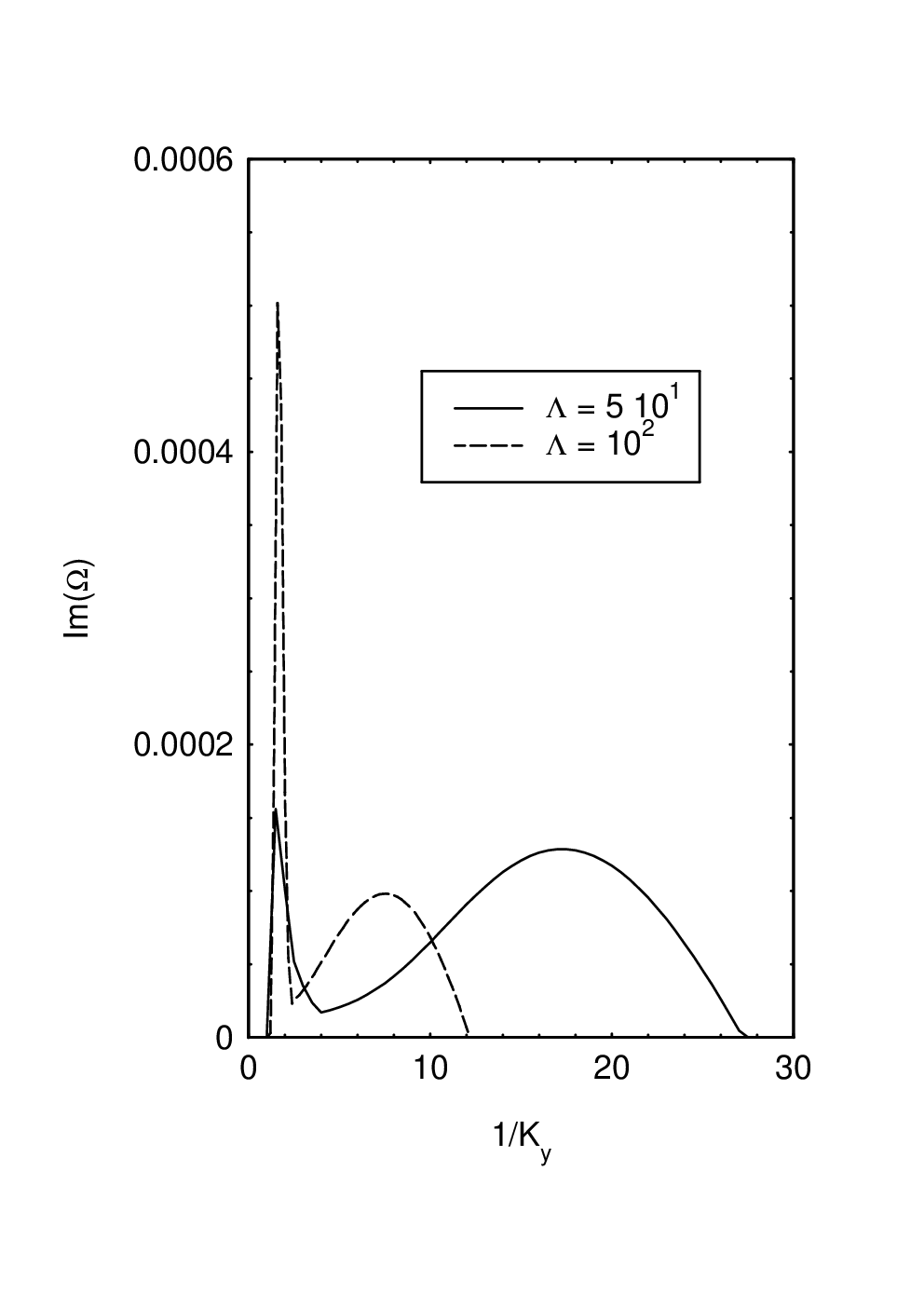
The maximum value of the instability increases and narrows with the state of charge of the dust $Z_{D}$ but decreases and get wider with the mass. For typical laboratory light dusty plasmas ($m_{d}\sim 10^{4}m_{p}$, $Z_{D}\sim 10^{3}$) the instability of dust acoustic or electrostatic waves is narrower and smaller than that for ions In figure 1 the peak of the left corresponds to the typical shape of instability of slightly inhomogeneous plasmas, while the right region of instability appears for density gradient lengths of the order of a hundred of Debye lengths ($\Lambda_{n}\equiv\Lambda\lesssim 10^{2}$). For higher density gradients ($\Lambda=5\times 10^{1}$), this new instability region is wider and so high as the typical one. For even higher density gradients ($\Lambda=10^{1}$), figure 2 shows that the new right region gives a higher instability. This figure also shows the effect of the non ideality of the plasma. necessary condition for the exhibition of dust acoustic waves. For typical laboratory dust radius the $b_{od}$ parameter of the hard core potential equation of state, is of the order of $10^{-14}m^{3}$. And for typical values of ion density of $10^{16}m^{-3}$ (and corresponding $n_{od}$, by quasi-neutrality relation), it appears a new intermediate instability region which can reach a maximum for denser plasmas ($n_{oi}=10^{17}m^{-3}$) or larger dust particles ($b_{od}\gtrsim 10^{-13}m^{3}$). This maximum is limited for the relation for dust collective behavior

$$r_{d}\ll\lambda_{Di}$$

(21)

1. 1.

   J. H. Chen, J. B. Du, and Lin I., J. Phys. D: Appl. Phys. 27, 296(1994)

2. 2.

   A. Barkan, R. L. Merlino, and N. D’Angelo, Phys. Plasmas, 2, 3563(1995)

3. 3.

   Reichl L.E., ”A Modern Course in Statistical Physics”, Edward Arnold, 1991.

4. 4.

   N. N. Rao, ”Frontier in Dusty Plasmas”, Y. Nakamura, T. Yakota, and P.K. Shukla, Eds., Elsevier Science B.V,(2000)

5. 5.

   F. H. Ree and W. G. Hoover, J. Chem. Phys, 40, 939(1964)

6. 6.

   P. Martín et al., J. Math. Phys. 21, 280 (1980)

7. 7.

   Mikhailovsky A. B., ”Handbook of Plasma Physics”, Rosenbluth and Sagdeev Eds., North Holland, Amsterdam, 1983.

8. 8.

   A. Galeev et al. Soviet Physics. JETP 17, 615 (1963)

9. 9.

   J. Puerta and C. Cereceda, Proc. ICPPP 1, 94 - 97 (1996)