Frozen light in periodic stacks of anisotropic layers
Abstract
We consider a plane electromagnetic wave incident on a periodic stack of dielectric layers. One of the alternating layers has an anisotropic refractive index with an oblique orientation of the principal axis relative to the normal to the layers. It was shown recently that an obliquely incident light, upon entering such a periodic stack, can be converted into an abnormal axially frozen mode with drastically enhanced amplitude and zero normal component of the group velocity. The stack reflectivity at this point can be very low, implying nearly total conversion of the incident light into the frozen mode with huge energy density, compared to that of the incident light. Supposedly, the frozen mode regime requires strong birefringence in the anisotropic layers – by an order of magnitude stronger than that available in common anisotropic dielectric materials. In this paper we show how to overcome the above problem by exploiting higher frequency bands of the photonic spectrum. We prove that a robust frozen mode regime at optical wavelengths can be realized in stacks composed of common anisotropic materials, such as , , , and the like.
I Introduction
In photonic crystals, the speed of light is defined as the wave group velocity, ,
| (1) |
where is the Bloch wave vector and is the respective frequency. At certain frequencies, the dispersion relation of a photonic crystal develops stationary points
| (2) |
in the vicinity of which the group velocity vanishes. Zero group velocity usually implies that the respective Bloch eigenmode does not transfer electromagnetic energy. Indeed, with certain reservations, the energy flux of a Bloch mode is
| (3) |
where is the electromagnetic energy density, associated with this mode. If is limited, then the group velocity and the energy flux vanish simultaneously at any stationary point (2) of the dispersion relation. Such modes are commonly referred to as slow modes, or slow light. Examples of different stationary points (2) are shown in Fig. 1., where each of the respective frequencies , , and is associated with slow light.

A common problem with slow modes is that most of them cannot be excited in semi-infinite photonic crystal by incident light. Indeed, consider plane monochromatic wave incident on a semi-infinite photonic crystal with the electromagnetic dispersion relation shown in Fig. 1. If the frequency is close to the band edge frequency in Fig. 1, then the incident wave will be totally reflected back into space, as seen in Fig. 2.

In another case, where the incident wave frequency is close to the characteristic value or in Fig. 1, some portion of the incident wave will be transmitted in the photonic crystal, but none in the form of the slow mode corresponding to the respective stationary point. This means, for example, that at the frequency , the transmitted light is a Bloch wave with the finite group velocity and the wave number different from that corresponding to the point in Fig. 1.
Let us turn now to the stationary inflection point of the dispersion relation in Fig. 1, where both the first and the second derivatives of the frequency with respect to vanish, while the third derivative is finite
| (4) |
The frequency of stationary inflection point is associated with the so-called frozen mode regime PRE01; PRB03; PRE03. In such a case, the incident plane wave can be transmitted into the photonic crystal with little reflection, as seen in Fig. 2. Having entered the photonic slab, the light is 100% converted into the slow mode with infinitesimal group velocity and drastically enhanced amplitude. Under the frozen mode regime, vanishingly small group velocity in Eq. (3) is offset by a huge value of the energy density . As the result, the energy flux (3) associated with the frozen mode remains finite and comparable with that of the incident wave. In the vicinity of the frozen mode frequency , the electromagnetic energy density associated with the slow (frozen) mode displays a resonance-like behavior
| (5) |
where is the fixed energy flux of the incident wave, is the portion of the incident light transmitted into the semi-infinite photonic crystal, and
Remarkably, the transmittance at remains finite and may even be close to unity, as shown in Fig. 2. The latter implies that a significant portion of the incident light is converted into the frozen mode with nearly zero group velocity and huge amplitude, compared to that of the incident wave. In reality, the electromagnetic energy density of the frozen mode will be limited by such factors as absorption, nonlinear effects, imperfection of the periodic dielectric array, deviation of the incident radiation from a perfect plane monochromatic wave, finiteness of the photonic slab dimensions, etc. Still, with all these limitations in place, the frozen mode regime can be very attractive for various practical applications.
From now on we restrict ourselves to the case of lossless periodic layered media (periodic stacks), which can be viewed as one dimensional photonic crystals. According to PRB03, at normal incidence, the frozen mode regime in a periodic stack can only occur if some of the layers display sufficiently strong circular birefringence (Faraday rotation). In addition, each unit cell of the periodic layered array must contain at least two layers with significant and misaligned in-plane anisotropy. If the above conditions are not met, the electromagnetic dispersion relation of the periodic stack cannot develop stationary inflection point (4) and, therefore, cannot support the frozen mode regime at normal incidence. At the microwave frequency range, one can find a number of materials meeting the above requirements. But at infrared and optical frequencies, the circular birefringence of known transparent magnetic materials becomes too small to support a robust frozen mode regime PRB03. Since our prime interest here is with optics, we will explore the ”non-magnetic” approach proposed in PRE03.
According to PRE03, the frozen mode regime can occur in nonmagnetic periodic stacks with special configurations requiring some layers to display appreciable oblique (neither in-plane, nor axial) anisotropy. On the other hand, at optical frequencies, all commercially available anisotropic dielectrics display substantially weaker anisotropy, compared to what would be the optimal value. According to PRE03, too weak anisotropy can push the frozen mode frequency too close to the nearest band edge, resulting in almost total reflectance of the incident light. The high reflectance of the slab, in turn, implies very low efficiency of conversion of the incident light into the slow mode. In this paper we show that in fact, the negative effect of the weak anisotropy on the frozen mode regime can be completely overcome by proper design of the layered structure. As the result, a robust frozen mode regime at optical frequencies can be achieved in periodic stacks incorporating real anisotropic materials such as yttrium vanadate, lithium niobate, and the like, where the dielectric anisotropy is one-two orders of magnitude short of the ”optimal” value. The idea is to choose the parameters of the periodic stack so that a stationary inflection point associated with the frozen mode regime develops at higher photonic bands. For a given frequency range, this requires thicker dielectric layers, which could be an additional practical advantage. A side effect of using higher photonic bands is that the effective bandwidth of the frozen mode regime appears to be narrower, compared to the case of hypothetical materials with much stronger anisotropy used in PRE03 for numerical simulations.
The practical development of frozen mode devices from such commodity materials could lead to revolutionary advances in optical computing, sensing, and information processing. When practically realized, such frozen mode structures would enable significant advances in all-optical information storage and processing (such as optical memory and buffer elements, optical delay lines) as well as optical sensing, lasing, and nonlinear optics.
The paper is organized as follows. In the next section, we discuss in general terms the phenomenon of axially frozen mode. The detailed analysis of the mathematical aspects of the phenomenon can be found in PRE03. Then, in section III, using a specific example of a periodic array incorporating yttrium vanadate, we demonstrate how a robust frozen mode regime at optical frequencies can be achieved in a practical setting involving weakly anisotropic materials. Finally, in Appendix, we briefly overview the electrodynamics of lossless layered media, introducing basic notations, definitions, and assumptions used in our computations.
II Axially frozen mode regime at oblique incidence
According to PRB03; PRE03, in nonmagnetic periodic stacks, the simplest version of the frozen mode regime described in the introduction is impossible. Still, a more general phenomenon referred to as the axially frozen mode regime can occur. This section starts with a brief general discussion of the phenomenon. Then we turn to the particular case of a periodic stack incorporating yttrium vanadate layers. The reason we have chosen this particular material is because its optical properties is very similar to those of other common anisotropic dielectrics transparent at optical wavelength.
II.1 Basic definitions
Consider a monochromatic plane wave obliquely incident on a periodic semi-infinite stack, as shown in Fig. 3.

Let , and denote the incident, reflected and transmitted waves, respectively. Due to the boundary conditions (46), all three waves , and must be assigned the same pair of tangential components of the respective wave vectorLLEM 84; Yariv
| (6) |
while their axial (normal) components can be different. Hereinafter, the symbol will refer only to the transmitted Bloch waves propagating inside the semi-infinite slab
| (7) |
The value is defined up to a multiple of (the Brillouin zone), where is the period of the layered structure. For given and , the value is found by solving the time-harmonic Maxwell equations (37) in periodic medium, that will be done in the following sections. The result can be represented as the axial dispersion relation, which gives the correspondence between and at fixed
| (8) |
It can be more convenient to define the axial dispersion relation as the correspondence between and at fixed direction of incident light propagation
| (9) |
where the unit vector can be expressed in terms of the tangential components (6) of the wave vector
| (10) |
Examples of axial dispersion relation (9) are presented in Figs. 5 and 6.


The transmitted electromagnetic field inside the periodic layered medium is not a single Bloch mode, but it is a superposition of two Bloch modes with different polarizations and different values of . Of course, the tangential components are the same for either transmitted Bloch mode and the incident wave, as stated by Eq. (6). Generally, there are three possibilities (see the details in PRE03):
- 1.
Both Bloch components of the transmitted wave are propagating modes, which means that the respective values of are real. For example, at and in Fig. 6 we have two Bloch modes propagating inside the slab with two different group velocities (double refraction). Note that propagating modes with , as well as evanescent modes with , do not contribute to the transmitted wave inside the semi-infinite stack in Fig. 3.
- 2.
Both Bloch components of are evanescent, which implies that the respective values of are complex with . In particular, this is the case if the frequency falls into a photonic band gap (for example, at in Fig. 1). In such a case, the incident wave is totally reflected back to space.
- 3.
Of particular interest is the case when one of the Bloch components of the transmitted wave is a propagating mode (with ), while the other is an evanescent mode (with )
(11) This is the case at the frequency range
(12) in Fig. 6. As the distance from the slab/vacuum interface increases, the evanescent contribution decays as , and the resulting transmitted wave turns into a single propagating Bloch eigenmode .
Similarly to the case (4) of regular frozen mode, the axially frozen mode is associated with the axial stationary inflection point defined as
| (13) |
The regular stationary inflection point (4) is a particular case of (13). Example of axial dispersion relation displaying such a singularity is shown in Fig. 6. In the vicinity of in Eq. (13), the electromagnetic field inside the slab is a superposition (11) of one propagating and one evanescent Bloch components. As the frequency approaches the critical point (13), both contributions grow sharply, while remaining nearly equal and opposite in sign near the slab boundary (at ), as illustrated in Fig. 7.

Due to the destructive interference at the slab boundary, the resulting electromagnetic field at is small enough to satisfy the boundary condition (46). As the distance from the slab boundary increases, the evanescent component decays exponentially, while the amplitude of the propagating component remains constant and large, as shown in Figs. 8b and 8c.

II.2 Energy density and energy flux of the axially frozen mode
Let , and be the energy fluxes of the incident, reflected and transmitted waves, respectively. Within the frequency range (12), which includes the critical point (13), the transmitted wave is a superposition (11) of propagating and evanescent components. Only the propagating component is responsible for the axial energy flux .
The axial energy flux can also be expressed in terms of the axial component of the propagating mode group velocity and the energy density associated with
| (14) |
The quantity in Eq. (14) can be interpreted as the electromagnetic energy density far from the slab interface, where the electromagnetic field reduces to its propagating component . In the vicinity of the axial stationary inflection point (13), the energy density , associated with the axially frozen mode, diverges, while . As a result, the vanishingly small in Eq. (14) is offset by a very large value of . The theoretical analysis of the next section shows that the axial energy flux in Eq. (14), along with the slab transmittance in (69), remain finite even at , where the axial component of the group velocity vanishes
| (15) |
The energy conservation consideration allows to find the asymptotic frequency dependence of the amplitude of the axially frozen mode in the vicinity of the critical point (13). Indeed, in the vicinity of , the axial dispersion relation can be approximated by a cubic parabola
| (16) |
The component of the group velocity is
| (17) |
The Eq. (17) together with (14) yield the following asymptotic expression for the energy density associated with the frozen mode
| (18) |
or, equivalently,
| (19) |
where is the fixed energy flux of the incident wave and is the transmittance coefficient defined in (69). Remarkably, the transmittance of the semi-infinite slab remains finite in the vicinity of the frozen mode frequency , as seen in Figs. 9 and 10. This implies that the electromagnetic energy density associated with the frozen mode, as well as its amplitude , diverge as . In Figs. 9 and 10 such a behavior is illustrated for two different incident light polarizations.


In reality, under the axial frozen mode regime, the field amplitude inside the slab is limited by various physical factors mentioned earlier in this paper. Still, with all these limitations in place, the normal energy flux remains finite and comparable with that of the incident wave. The latter implies that a substantial portion of the incident wave is converted into the axially frozen mode with drastically enhanced amplitude and nearly zero axial component of the group velocity. In many respects, the phenomenon of axial frozen mode is similar to its particular case, the regular frozen mode, associated with the regular stationary inflection point (4).
II.3 Physical conditions for the axially frozen mode regime in layered media
The physical conditions under which a non-magnetic layered structure can support the (axial) frozen mode regime can be grouped in two categories. The first one comprises several symmetry restrictions. The second category includes some basic qualitative recommendations which would ensure the robustness of the frozen mode regime, provided that the symmetry conditions for the regime are met. In what follows we briefly reiterate those conditions and then show how they apply to periodic stacks incorporating some real dielectric materials.
II.3.1 Symmetry conditions
There are two fundamental necessary conditions for the frozen mode regime. The first one is that the Bloch dispersion relation in the periodic layered medium must display the so-called axial spectral asymmetry
| (20) |
As shown in PRE03, this condition is necessary for the existence of the axial stationary inflection point (13) in the electromagnetic dispersion relation of an arbitrary periodic layered medium.
The second necessary condition is that for the given direction of wave propagation, the Bloch eigenmodes with different polarizations must have the same symmetry. In the case of oblique propagation in periodic layered media, the latter condition implies that for the given , the Bloch eigenmodes are neither TE nor TM
| (21) |
The condition (20) imposes certain restrictions on (i) the point symmetry group of the periodic layered array and (ii) on the direction of the transmitted wave propagation inside the layered medium. While the condition (21) may impose some additional restriction on the direction of .
The restriction on the symmetry of the periodic stack following from the requirement (20) of the axial spectral asymmetry is
| (22) |
where is the mirror plane parallel to the layers, is the 2-fold rotation about the axis. An immediate consequence of the criterion (22) is that least one of the alternating layers of the periodic stack must be an anisotropic dielectric material with nonzero and/or , where the direction is normal to the layers
| (23) |
Otherwise, the operation will be present in the symmetry group of the periodic stack.
The condition (20) also imposes a restriction on the direction of wave propagation. Specifically, the Bloch wave vector must be oblique to the stack layers, which means that is neither parallel, nor perpendicular to the direction
The latter condition implies that the frozen mode regime cannot occur at normal incidence, regardless of the periodic stack geometry and composition. While the condition (23) implies that at least one of the alternating layers must be cut at an oblique angle relative to the principle axes of its permittivity tensor. If either of the above two conditions is not satisfied, the dispersion relation will be axially symmetric
| (24) |
which rules out the possibility of stationary inflection point and the frozen mode regime.
II.3.2 Additional physical requirements
In practice, as soon as the symmetry conditions are met, one can almost certainly achieve the (axial) frozen mode regime at any desirable frequency within certain frequency range. The frequency range is determined by the layers thicknesses and the dielectric materials used, while a specific value of within the range can be selected by the direction of the light incidence. The problem is that unless the physical parameters of the stack layers lie within a certain range, the effects associated with the frozen mode regime can be insignificant or even practically undetectable. The basic guiding principle in choosing appropriate layer materials is ”moderation”. As soon as the ”moderation” principle is observed, one can almost certainly achieve the frozen mode regime at prescribed frequency by choosing the right direction of light incidence. Specifically, those ”moderation” conditions include:
- 1.
It is desirable that the ratio
(25) of the birefringence and the refractive index of the material of the anisotropic layers lies somewhere between 2 and 10. If the anisotropy is extremely strong or too weak, the Bloch waves with different polarizations become virtually separated, which excludes the possibility of a robust frozen mode regime. For example, in the practically important case of extremely small anisotropy, the two transmitted Bloch waves can be approximately classified as TE and TM modes, which is incompatible with the symmetry condition (21) for the frozen mode regime.
- 2.
The dielectric contrast of the adjacent layers and should be significant, but not extreme. The ratio anywhere between 1.5 and 20 would be appropriate. In addition, the dielectric contrast between the layers should match the ratio (25) in the anisotropic layers: weaker anisotropy would require weaker dielectric contrast between the layers.
- 3.
Typical layer thickness should be of the order of , where is the light wavelength in vacuum and is the respective refractive index. In reality, the acceptable layer thickness can differ from by several times either way. But too thick layers would push the stationary inflection point to high-order frequency bands, while too thin layers would exclude the possibility of the frozen mode regime at the prescribed frequency range.
The biggest challenge at optical frequencies poses the first condition, because most of the commercially available optical anisotropic crystals have the ratio of only about 0.1. According to PRE03, this would push the axial stationary inflection point (13) very close to the photonic band edge and make the photonic crystal almost 100% reflective. This indeed would be the case if we tried to realize the frozen mode regime at the lowest frequency band. But, in the next section we show that one can successfully solve this problem by moving to a higher frequency band. So, a robust axially frozen mode regime with almost complete conversion of the incident light into the frozen mode can be achieved with the commercially available anisotropic dielectric materials displaying the birefringence ratio (25) by one-two orders of magnitude smaller, compared to the optimal value used in PRE03 for numerical simulations. The drawback though is that using higher photonic frequency bands narrows the bandwidth of the frozen mode regime by roughly an order of magnitude.
III Periodic stack incorporating Yttrium Vanadate layers
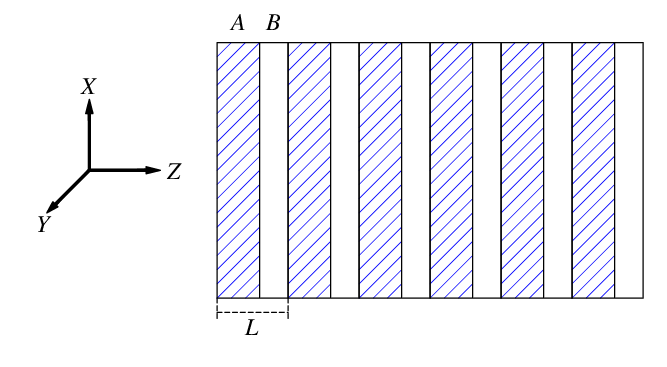
The simplest non-magnetic periodic stack satisfying the symmetry conditions (22) and (23) and, therefore, capable of supporting the axial frozen mode regime, is shown in Fig. 4. It is composed of anisotropic layers separated by empty gaps. The anisotropic dielectric layers must display nonzero components and/or . The simplest choice for the respective permittivity tensor is
| (26) |
where the axis coincides with the normal to the layers.
Yttrium vanadate is a tetragonal dielectric with the permittivity tensor, , at nm eps
| (27) |
where the Cartesian axis is chosen parallel to the crystallographic axis . In order to achieve a non-zero component one has to rotate the tensor (27) about the axis by an angle , different from and Ballato. The result of the rotation is
| (28) |
For numerical simulations we can choose, for instance,
| (29) |
In this case, Eq. (28) together with (27) yield
| (30) |
which is compatible with the required form (26).
Let and denote the thickness of the layers and the thickness of the gaps between them, respectively. For our numerical simulations we can choose
| (31) |
where is the period of the layered array in Fig. 4.
Let us reiterate that the parameters (29) and (31) are chosen at random. In practice, we can always adjust them so that the stack suits specific practical requirements. The structural period should be chosen so that the frozen mode regime occurs within a prescribed frequency range. Then, the direction of light incidence can be adjusted so that the axial frozen mode regime occurs exactly at a prescribed frequency .
Symmetry arguments similar to those presented in PRE03 show that in the case of the periodic array in Fig. 4, the necessary conditions (22) and (21) for the frozen mode regime are satisfied only if the direction of the light incidence lies neither in the , nor plane
| (32) |
III.1 Electromagnetic properties in the vicinity of axial frozen mode regime
In Fig. 5 we presented the typical axial dispersion relation of the periodic stack in Fig. 4 at fixed direction of light incidence. In Fig. 5 we chose
| (33) |
because this particular direction of light incidence produces the axially frozen mode regime at certain frequency , shown in Fig. 6. Due to the relatively small anisotropy of yttrium vanadate, the axial dispersion relation in Fig. 5 displays rather weak asymmetry , which makes it virtually impossible to develop a stationary inflection point at the lowest spectral branches. As we go to upper photonic bands, the situation improves. In Fig. 6 we present the enlarged fragment of the axial dispersion relation in Fig. 5. This fragment covers the boundary region between the forth and the fifth bands. At frequency
| (34) |
one of the spectral branches develops axial stationary inflection point (13), associated with the possibility of the axial frozen mode regime.
Our numerical analysis based on the transfer matrix approach (the computational details are presented in the next section) indeed shows a very robust (axial) frozen mode regime in this setting, in spite of the fact that the dielectric anisotropy of yttrium vanadate is more than an order of magnitude short of the optimal value. The drawback though is that the frequency bandwidth of the effect is roughly an order of magnitude narrower, compared to what could be achieved with hypothetical materials displaying much stronger anisotropy at optical frequencies.
Let us start with the results presented in Figs. 9 and 10. The bottom plots in both figures display the frequency dependence of the stack transmittance for two different polarizations of incident light . Clearly, in the vicinity of the frozen mode frequency , the transmittance remains significant, which implies that a significant portion of the incident radiation is converted into the frozen mode. The top plots in Figs. 9 and 10 display the amplitude of the two Bloch components of the transmitted wave . The solid and dotted lines correspond to the propagating and evanescent Bloch components, respectively. In the vicinity of the frozen mode frequency (at ), there is one propagating component () and one evanescent component (), each of which diverges as , in accordance with Eq. (19). At and , the transmitted wave is a superposition of two propagating components with different group velocities, which constitutes the phenomenon of double refraction. The characteristic frequencies in Figs. 9 and 10 are explained in Fig. 6.
Fig. 7 shows the frequency dependence of the resulting field amplitude at the slab boundary, along with the amplitudes of its propagating and evanescent components and . Although each of the two Bloch contributions to diverges as , their superposition remains finite, to meet the boundary conditions (46) at . As we move further away from the slab boundary, the evanescent component dies out, while the propagating mode remains constant and large. As a result, the destructive interference of and is removed, and the resulting field amplitude grows and approaches the value . This scenario is illustrated in Fig. 8b and 8c. If the frequency of the incident wave and its direction of propagation exactly correspond to the critical values and , then the electromagnetic field inside the semi-infinite stack is described by a linearly diverging non-Bloch Floquet eigenmode
as shown in Fig. 8a.
By way of example, let us present the actual geometrical parameters of the stack supporting the axially frozen mode regime for the case of infrared light with nm and the direction of incidence (33). The expression (34) for the frozen mode frequency yield
In practice, we do not have to adjust the layer thicknesses in order to achieve the frozen mode regime at a prescribed wavelength. Instead, we can tune the system into the axially frozen mode regime by adjusting the direction of light incidence.
Acknowledgments. The effort of A. Figotin and I. Vitebskiy was supported by the U.S. Air Force Office of Scientific Research under the grant FA9550-04-1-0359. The authors (JB) also wish to thank the Defense Advanced Research Projects Agency (DARPA) for support under grant N66001-03-1-8900 through SPAWAR.
References
- (1) A. Figotin, and I. Vitebsky. Nonreciprocal magnetic photonic crystals. Phys. Rev. E63, 066609 (2001).
- (2) A. Figotin, and I. Vitebskiy. Electromagnetic unidirectionality in magnetic photonic crystals. Phys. Rev. B67, 165210 (2003).
- (3) A. Figotin, and I. Vitebskiy. Oblique frozen modes in layered media. Phys. Rev. E68, 036609 (2003)
- (4) L. D. Landau, E. M. Lifshitz, L. P. Pitaevskii. Electrodynamics of continuous media. (Pergamon, N.Y. 1984)
- (5) A. Yariv and P. Yeh. Optical Waves in Crystals. (”A Wiley-Interscience publication”, 1984)
- (6) Pochi Yeh. ”Optical Waves in Layered Media”, (Wiley, New York, 1988).
- (7) Amnon Yariv and Pochi Yeh. ”Optical waves in crystals: propagation and control of laser radiation”, (New York, Wiley, 1984).
- (8) Smithsonian Physical Tables, 9th Revised Edition, W. Forsythe, ed. (Knovel Publishing, Danbury, CT, 2003)
- (9) J. Ballato and A. Ballato. Materials for Freezing Light. Waves in Random Media (accepted 2004)
- (10) D. W. Berreman. J. Opt. Soc. Am. A62, 502–10 (1972).
- (11) I. Abdulhalim. Analytic propagation matrix method for linear optics of arbitrary biaxial layered media, J.Opt. A: Pure Appl. Opt. 1, 646 (1999).
- (12) I. Abdulhalim. Analytic propagation matrix method for anisotropic magneto-optic layered media, J.Opt. A: Pure Appl. Opt.2, 557 (2000).
IV APPENDIX. Scattering problem for anisotropic semi-infinite stack
In this section we briefly discuss the standard procedure we use to do the electrodynamics of stratified media incorporating anisotropic layers. For more details, see, for example, Tmatrix; Abdul99; Abdul00; PRE03 and references therein.
IV.1 Time-harmonic Maxwell equations in periodic layered media
Our consideration is based on time-harmonic Maxwell equations
| (35) |
with linear constitutive relations
| (36) |
In layered media, the tensors and in Eq. (36) depend on a single Cartesian coordinate . Plugging Eq. (36) into (35) yields
| (37) |
Solutions for Eq. (37) are sought in the following form
| (38) |
which is a standard choice for the scattering problem of a plane electromagnetic wave incident on a plane-parallel stratified slab. Indeed, in such a case, due to the boundary conditions (45), the tangential components of the wave vector are the same for the incident, reflected and transmitted waves. The substitution (38) in Eq. (37) allows to separate the tangential field components into a closed system of four linear differential equations
| (39) |
The matrix is referred to as the Maxwell operator. The reduced Maxwell equation (39) for the four tangential field components should be complemented with the following expressions for the normal components of the fields
| (40) |
where
| (41) |
The expression for the Maxwell operator is very cumbersome, its explicit form can be found in PRE03. The matrix elements of depend on the following parameters: the frequency , the direction of light incidence, the material tensors and .
In a periodic layered medium
| (42) |
where is the stack period. For any given , and , the system (39) of four ordinary linear differential equations with periodic coefficients has four Bloch solutions
| (43) |
where correspond to four solutions for for given , and
| (44) |
Real in (44) relate to propagating Bloch eigenmodes, while complex relate to the evanescent modes. In the case of propagating eigenmodes, the correspondence between and for fixed is referred to as the axial dispersion relation, the concise form of which is given by Eqs. (8) or (9).
IV.2 Boundary conditions
The boundary conditions at the slab/vacuum interface reduce to the continuity requirement for the tangential field components at
| (45) |
where the indices , and denote the incident, reflected and transmitted waves, respectively. Using representation (38), we can recast (45) in a compact form
| (46) |
where
describe the incident and reflected waves, respectively. , , are the Cartesian components of the unit vector (10).
Knowing the eigenmodes (43) inside the slab and using the boundary conditions (46) we can express the amplitude and composition of the transmitted wave and reflected wave , in terms of the amplitude and polarization of the incident wave . This gives us the electromagnetic field distribution inside the layered medium, as well as the transmittance and reflectance coefficients of the semi-infinite slab as functions of the incident wave polarization, the direction of incidence, and the frequency .
IV.3 Energy flux, reflectance, transmittance
The real-valued Poynting vector is defined by
| (63) |
Plugging the representation (38) for and in Eq. (63) yields
| (64) |
implying that none of the three Cartesian components of the energy density flux depends on the tangential coordinates and . In addition, the energy conservation argument implies that the axial component of the energy flux does not depend on the coordinate either
| (65) |
This only apply to the case of a plane monochromatic wave incident on a lossless layered medium. The explicit expression for the component of the energy flux (64) is
| (66) |
Let us turn to the scattering problem for semi-infinite slab. Let , and be the Poynting vectors of the incident, reflected and transmitted waves, respectively. The energy conservation imposes the following relation between the normal components of these three vectors
| (67) |
Since the stack is presumably composed of lossless materials, the component of the energy flux is independent of coordinates both inside and outside the stack. In particular, inside the slab we have
| (68) |
The transmittance and the reflectance of a lossless semi-infinite slab are defined as
| (69) |