Hyperfine Spectroscopy of Optically Trapped Atoms
Abstract
We perform spectroscopy on the hyperfine splitting of 85Rb atoms trapped in far-off-resonance optical traps. The existence of a spatially dependent shift in the energy levels is shown to induce an inherent dephasing effect, which causes a broadening of the spectroscopic line and hence an inhomogeneous loss of atomic coherence at a much faster rate than the homogeneous one caused by spontaneous photon scattering. We present here a number of approaches for reducing this inhomogeneous broadening, based on trap geometry, additional laser fields, and novel microwave pulse sequences. We then show how hyperfine spectroscopy can be used to study quantum dynamics of optically trapped atoms.
1 Introduction
The development of laser cooling and trapping techniques [1, 2, 3] has been motivated, to a great extent, by their potential use for precision measurements, of which precision frequency measurements are of outmost importance. Cold atoms are attractive for these measurements mainly because of the suppression of the Doppler broadening and because they allow for a longer interrogation time and hence a narrower linewidth.
Modern atomic frequency standards are based on atomic clocks, which measure the frequency associated with the transition between two ground state hyperfine levels. The performance of such a clock can be improved by lengthening the time over which such a transition is measured. During the 1950’s various possibilities were suggested to lengthen this interrogation time: Ramsey [4] proposed confining the atoms in a storage ring with an inhomogeneous magnetic field, or a storage cell with properly coated walls. Zacharias [5] proposed to build an atomic “fountain” in which a thermal beam of atoms is launched upward, so slow atoms from the tail of the velocity distribution will turn around and fall back under the force of gravity. Using the Ramsey method of separated fields, the atoms could be interrogated once on their way up and then again on their way down, resulting in a long total interrogation time. Back then, this idea failed because of collisions of these slow atoms with the faster ones. Using laser-cooled atoms, Zacharias’ idea was revived in 1989 by Kasevich et. al. [6]. They cooled sodium atoms using a magneto-optical trap [7] and launched them on ballistic trajectories by applying a short pulse of resonant light. Two short microwave pulses were applied as the atoms turned around inside a waveguide and allowed the ground-state hyperfine splitting to be measured with a linewidth of .
To further increase the measurement time beyond the practical limit imposed by the height of a fountain, one can use trapped atoms, and in particular optical dipole traps, based on the dipole potential created by the interaction of a neutral atom and a laser beam [8, 9]. Unfortunately, the interaction between the trapping light and the trapped atoms is not negligible. First, even for a far-off-resonance trap, where many of the undesired effects of the atom-light interaction are suppressed, residual spontaneous scattering of photons from the trap laser destroys the ground state spin polarization or spin coherence [10]. Next, and more importantly, atom trapping relies on inducing a spatial inhomogeneous shift of the atomic energy levels, and the existence of such a shift makes precision spectroscopy of trapped atoms a difficult task. In the case of hyperfine spectroscopy in optical traps, the inhomogeneity is approximately equal for both states, since the trapping light interacts with both levels with the same strength (the dipole matrix elements are identical). However, the difference in detuning between them results in a differential inhomogeneity, which induces a dephasing effect and, when ensemble-averaged, causes a broadening of the spectroscopic line and hence a loss of atomic coherence at a much faster rate than the spontaneous photon scattering rate [11]. These effects can be reduced by increasing the trap detuning [11, 12, 13, 14] and also by using blue-detuned optical traps, in which the atoms are confined mainly in the dark [11, 15]. However, the residual frequency shifts are still the main factor limiting the coherence of the trapped atoms, and hence the use of dipole traps for precision spectroscopy.
A number of approaches for reducing the inhomogeneous broadening of the ground state hyperfine splitting of optically trapped atoms are presented in this tutorial. Following a brief review on light shifts and optical dipole traps in section 2, and a description of the basic experimental setup in section 3, we present in section 4 a simple, classical model for microwave spectroscopy in an optical trap, and use it to analyze the atomic coherence times for different trap geometries in section 5. Based on this model, we present in section 6 a novel method for reducing the inhomogeneous frequency broadening by the addition of a weak light field, spatially mode-matched with the trapping field and whose frequency is tuned in-between the two hyperfine levels. In section 7 we show another way of achieving long coherence times in an optical trap: a narrow energy distribution is achieved using a microwave “pre-selection” pulse which selects a subset of the atomic ensemble. Our technique allows the selection of a narrow energy band around any central energy enabling us to maximize the number of selected atoms (for a given energy width) by choosing the energy with the highest density of populated states.
A full, quantum-mechanical model is developed in section 8. The limit of short and strong pulses is further elaborated in section 9, and used to predict the Ramsey decoherence time of a thermal ensemble as a consequence of dephasing. In section 10 it is shown that, for certain trap parameters, the dephasing can be reversed by stimulating a “coherence echo”. The failure of the echo for other trap parameters is due to dynamics in the trap, and thereby “echo spectroscopy” can also be used to study quantum dynamics in the trap even when more than 106 states are thermally populated, and to study the crossover from quantum dynamics to classical dynamics. We then show (in section 12) that the decay in the hyperfine coherence due to interactions with the environment, is only partly suppressed by echo spectroscopy, primarily due to dynamical (time-dependent) dephasing mechanisms. An improved pulse sequence is demonstrated, containing additional pulses for which the decay of coherence is reduced by a factor 2.5 beyond the reduction offered by the simple echo scheme.
Finally, in section 13 we show that our echo spectroscopy methods enable us to study quantum dynamics of trapped atoms also for chaotic and mixed dynamics where, surprisingly, partial revivals of atomic coherence occur in the perturbative (quantum) regime, and disappear in the non-perturbative (semi-classical) regime, indicating a clear quantum to classical transition as a function of the perturbation strength.
2 Light Shifts and Dipole Traps
Throughout the work presented in this tutorial we use far-off-resonance optical dipole traps, which are traps based on the dipole potential created by the interaction of a neutral atom and a laser beam [9]. A few concepts on which the rest of the work presented here is based, are reviewed. In sections 2.1 and 2.2 a brief review of the origin of the dipole potential, and its connection with the ac Stark shift of the ground-state is presented using an idealized two-level atom. In section 2.3 a short review on the use of the dipole potential to trap neutral atoms is given11 1 Laser-cooling of the atoms is a prerequisite for dipole trapping, and is done with techniques that have became standard in many research laboratories, and will not be reviewed here (See Refs. [16, 17, 18]).. In sections 2.4 and 2.5, a description of the main mechanisms for atomic decoherence is given, this time for multi-level atoms.
2.1 The Optical Dipole Potential
The interaction of a neutral atom and a nearly-resonant electro-magnetic field is governed by the dipole interaction, and is usually separated into two terms which correspond to a reactive force and a dissipative force. When an atom is exposed to light, the electric field component induces a dipole moment in the atom, oscillating at the driving-light frequency.
If we assume for example a monochromatic light field with an electric field given by , where is the unit polarization vector and the frequency, then the dipole moment is . The amplitude of the dipole moment is related to the amplitude of the field by , where is the atomic complex polarizability, which is a function of the driving frequency. The interaction of the induced dipole moment with the driving field gives rise to the potential [9]
| (1) |
where is the light intensity. The reactive “dipole” force is a conservative one, and is equal to the gradient of the above potential. The dissipative force is related to the power the oscillating dipole absorbs from the field, which is given by:
| (2) |
In a quantum picture, the dipole force results from absorption of a photon from the field followed by stimulated emission of a photon into a different mode of the laser field. The momentum transfer is the vector difference between the momenta of the absorbed and emitted photons. The dissipative component has its origin in cycles of absorption of photons, followed by spontaneous emission, in a random direction. Using equation 2 we can write an equation for the rate of spontaneous photon scattering:
| (3) |
The atomic polarizability can be calculated by using the solutions of the optical Bloch equations, while translational degrees of freedom are taken into account [19]. For a two-level atom with resonance frequency , and using the “rotating wave approximation”, the average dipole potential can be written as
| (4) |
The resulting expression for the average scattering rate is
| (5) |
where is the natural linewidth of the atomic transition, is the detuning of the laser from the atomic resonance, is the saturation intensity of the transition, given by , and . For a large detuning from resonance () equations 4 and 5 can be approximated as
| (6) | |||||
| (7) |
2.2 Ground State Light Shifts

It is useful to look at the atom-light interaction in the “dressed state” model [19]. The combined Hamiltonian for the atom and the laser field is given by , where ,, and are the atom, laser and interaction parts of the Hamiltonian, respectively. Consider a two-level atom with ground state and excited state with energy , in the presence of a laser with frequency . The atom can be described by the Hamiltonian
| (8) |
and the laser field by
| (9) |
where and are the photon creation and annihilation operators, respectively. If the coupling between the atom and the field is ignored, then the eigenstates of are characterized by the atomic internal state (either or ) and by the number of photons in the electromagnetic field, . The energy levels form a ladder of manifolds, separated by , each containing two states of the form and (see figure 1a). If the light is in resonance with the atomic transition, these two states are degenerate. Otherwise, they are separated by .
A general result from second-order time-independent perturbation theory is that an interaction Hamiltonian will lead to a shift in the energy of the (unperturbed) -th state given by [9]
| (10) |
The interaction term in our case is , where is the electric dipole operator. This interaction term couples states within the same manifold with a matrix element given by
| (11) |
where is the Rabi frequency. The eigenfunctions of the coupled system, denoted “dressed states”, are a mixture of the uncoupled system eigenstates and are given by [18]
| (12) | |||
| (13) |
where . The new (dressed) levels are separated by an energy , where is called the “generalized Rabi frequency”. For a large detuning, , the ground state is shifted by (see figure 1b). The dressed states ,, … can be identified with the original ground state, with a small mixture of the excited state. This light-induced shift in the atomic energy levels is usually denoted “light shift” or “ac Stark shift”. Using , where is the saturation intensity of the transition, we conclude that the light-shift of the ground state energy, , is given by
| (14) |
As seen, in the perturbative limit the light-shift of the ground state is equal to the dipole potential in equation 6. The reason is that, since in this regime the atom is mostly in the ground state, the light shifted ground state can be identified as the potential for the motion of the atoms (see figure 1c). In the case of multi-level atoms, equation 14 should be modified to include the electric dipole interaction between the ground-state and all the excited states, with their respective detuning and transition strength (see section 2.5).
2.3 Optical Dipole Traps
The dissipative part of the atom-light interaction is used for laser cooling of atoms [16], a pre-requisite for optical trapping. However, spontaneous photon scattering is in general detrimental to trapped atoms, mainly because it can induce heating and loss. Comparing equations 6 and 7 yields,
| (15) |
which results in the well known fact that a trap with an arbitrarily small scattering rate can be formed by increasing the detuning while maintaining the ratio .
Equation 6 indicates that if the laser frequency is smaller than the resonance frequency, i.e. (“red-detuning”) the dipole potential is negative and the atoms are attracted by the light field. The minima of the potential is found then at the position of maximum intensity. In the case (“blue detuning”) the minima of the potential is located at the minima of the light intensity.
Trapping atoms with optical dipole potentials was first proposed by Letokhov [20] and Ashkin [21] . Chu and coworkers [8], were the first to realize such a trap, trapping about 500 atoms for several seconds using a tightly focused red-detuned beam. Later, a far-off-resonant trap for rubidium atoms was demonstrated [13], with a detuning of up to 65 nm, i.e. . In this case, the potential is nearly conservative and spontaneous scattering of photons is greatly reduced. A comprehensive review of the different schemes and applications of such optical dipole traps is presented in reference [9]. In the limiting case where the frequency of the trapping light is much smaller then the atomic resonance, trapping is still possible, practically with no photon scattering [22]. Such a quasi-electrostatic trap, formed by two crossed CO2 laser beams, was used to create a Bose-Einstein condensate without the use of magnetic traps [23].
Apart from using far-off-resonance lasers, the interaction between the light field and the atoms can be reduced by the use of blue-detuned traps, in which atoms are confined mostly in the dark [15]. Experimentally, blue-detuned traps, which require surrounding a dark region of space with a repulsive dipole potential, are harder to realize than red-detuned ones, where already a single focused beam constitutes a trap [8]. Several configurations for far-detuned dark optical traps were demonstrated, in which gravity provided the confinement in one direction: “Light sheets” traps were generated by elliptically focusing two laser beams and overlapping the two propagating light sheets to form a “V” cross-section that supports against gravity, while the confinement in the laser propagation direction is provided by the beam divergence [11]. In a later work, and in order to achieve larger trapping volume, a different trap was constructed with four light sheets producing an inverted pyramid [24]. A single beam trap was demonstrated using two axicons and a spherical lens to generate a conical hollow beam propagating upwards [25]. Such gravito-optical traps are limited to weak confinement. Traps in which light provided the confinement in all directions were developed with hollow beams. Laguerre-Gaussian “doughnut” modes were used, together with additional plug-in beams, to form such a trap [26].
Several dark traps based on a single laser beam were demonstrated, providing grater experimental simplicity and enabling dynamical changes of the trap geometry and strength. As opposed to the 2D case, were any desired light distribution can be generated using diffractive or refractive optical elements, there is no simple procedure to design an arbitrary 3D light distribution [27, 28]. Nevertheless, through the use of refractive and holographic optical elements, it is possible to produce light distributions which are suitable for trapping atoms in the dark using a single laser beam. Such light distributions, which comprise of a dark volume completely surrounded by light, were realized using either combinations of axicons and spherical lenses, diffractive optical elements, or rapidly scanning laser beams.
In the first scheme realized, the trapping beam was produced by passing a Gaussian beam through a phase plate of appropriate size, which shifted the optical phase at the center of the beam by radians. Interference leads to a dark volume at the focus of the lens, surrounded by light in all directions [29]. An additional method, with a much larger volume and more symmetric shape, was realized by simultaneously focusing two diffraction orders of a properly designed binary phase element, consisting of concentric phase rings with a -phase difference between subsequent rings [30]. An improved trap configuration was demonstrated by adding an axicon telescope before the phase element of the above setup [31]. This configuration maximizes the trap depth for a given laser power and trap dimensions, and greatly reduces the light induced perturbations to the trapped atoms. A related scheme was demonstrated in references [32] and [33]. Finally, a tightly-focused rapidly-rotating laser beam was used to create a trap [34]. If the scan frequency is high enough, the optical dipole potential can be approximated as a time averaged quasi-static potential. For a blue-detuned laser beam, and a radius of rotation larger than the waist of the focussed beam, a dark volume suitable for 3D trapping is obtained.
2.4 Photon Scattering and Coherence Relaxation in Multi-Level Atoms
The dipole potential can be viewed as originating from cycles of absorption of a photon and stimulated emission into a different laser mode. This process is unfortunately accompanied by spontaneous scattering, in which the absorption is followed by spontaneous emission in a random direction. Spontaneous scattering is one of the main limiting mechanism for the atomic hyperfine coherence22 2 A word of caution is in order about our use of the terms “decoherence” and “dephasing” . Decoherence results from the dissipative interaction of a single quantum superposition state with the environment (e.g. in the case of trapped atoms, the coupling to the electro-magnetic vacuum which leads to spontaneous scattering of photons). In addition, the response of a macroscopic ensemble of quantum systems (each prepared in a superposition state) decays due to the dephasing between the microscopic systems resulting from local variations in their evolution, and hence the ensemble coherence is lost..
Spontaneous scattering is a two-photon process, in which an atom initially at a state absorbs a photon from the trap laser and moves to an intermediate state of some excited level. The atom then decays back to the ground state, to a final state . If and , the process is called “Rayleigh scattering”. Otherwise, it is denoted “Raman scattering”. Clearly, Raman events destroy the atomic state coherence and hence are detrimental to the spectroscopy. As will be discussed below in section 12, also Rayleigh scattering events can be destructive for spectroscopy of a trapped ensemble.
The probability amplitude for scattering between and , via an intermediate state is proportional to , where () are the spherical components of the dipole moment operator ( or depending on the polarization of the absorbed and emitted photons). If the detuning from resonance is large enough such that no specific intermediate state is resolved, then to calculate the rate of transitions between and the amplitudes for all possible paths must be summed. For rubidium atoms, these are the two excited states and , with all their different hyperfine levels and corresponding Zeeman sub-levels. We further assume that the laser polarization is linear, hence conservation of angular momentum dictates . The total transition rate is [10]
| (16) |
where
| (17) |
Here and are the transition frequency and excited state lifetime of the line (), and is the amplitude for the strongest transition.
The first step in spectroscopy of trapped 85Rb atoms, is to transfer the entire population to . There, it is distributed uniformly between levels. We then apply a certain microwave pulse sequence (e.g. a Rabi pulse) which acts only on the transition , since a bias magnetic field is applied to shift all other transitions from resonance. Finally, we detect the total population of . We would like to measure, independently, the rate of incoherent scattering events that also affect the population of , in order to subtract them from our coherently driven population changes. Experimentally, we can measure the amount of -changing transitions, but not the rate of Rayleigh scattering events, or Raman events that do not change [10]. Equation 16, together with the appropriate summation, is used to calculate the relative amount of different scattering processes. For example, the rate for a transition between hyperfine levels and is calculated by averaging over initial levels of , and summing over final levels of . The total scattering rate is given by summing over levels of and levels of . Figure 2 shows a calculation of the relative amount of these two processes, as a function of the laser wavelength. Using the results of figure 2 we calculate the total amount of scattering events out of our measurement.

Note, that for a detuning larger than the fine-structure splitting of the excited state ( in rubidium), a destructive interference exists between the transition amplitudes for Raman scattering, summed over the intermediate excited states [10]. In this case, most spontaneous scattering events leave the internal state of the atom unchanged.
2.5 Light Shifts and Dephasing in Multi-Level Atoms
For a real multi-level atom, the light-shifts described in section 2.2 depend, in general, on the particular substate of the atom. The equivalent of equation 14 in the case of a multi-level atom can be written using the dipole matrix elements between a specific ground state and a specific excited state . Using , we can write the ac Stark shift for a ground state as [9]:
| (18) |
The summation takes into account the contributions of the different coupled excited levels , each with its respective transition coefficient , and detuning .
If the detuning of the light is large as compared to the excited state hyperfine splitting , then certain sum rules exist for the transition coefficients [35] and equation 18 for the shift of a ground state with total angular momentum , simplifies to:
| (19) |
where is the light polarization ellipticity and [] is the detuning of the laser from the [] line. For linearly polarized light ()
| (20) |
where
| (21) |
is the “weighted detuning” (below, we drop the “” and call this the detuning). Note, that the interaction matrix elements are identical for atoms in and . However, the light shift is inversely proportional to the trap laser detuning, which differs by , and therefore the potential from a far-detuned laser is slightly different for the two hyperfine levels. Loosely speaking, this difference in potential means that different hyperfine states “feel” different trap shapes. For microwave spectroscopy of a thermal ensemble this results in a rapid decay of the ensemble-averaged spectroscopic signal as a consequence of dephasing, much faster than the decay due to spontaneous scattering of photons.
3 Experimental Setup
All the experiments described in this tutorial consist of three stages. During the first stage standard laser-cooling techniques are used to cool an ensemble of 85Rb atoms and load a portion of them into a far-off-resonance trap. During the second stage, all the nearly-resonant laser beams are shut-off leaving only the far-off-resonance trapping beam on, and microwave pulses are applied. In last stage short pulses of on-resonance beams are used for the diagnostics. In this section, a detailed description of the above steps is provided.
3.1 Laser Cooling and Trapping
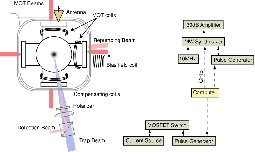
The heart of our setup is a vacuum chamber connected to a small reservoir of rubidium atoms through a valve. The chamber has six big windows used for the laser beams, and two additional small windows used for imaging the atomic cloud with an intensified CCD camera and measuring the fluorescence signal with a photomultiplier tube (see figure 3).
The first step in all the experiments described here is a magneto-optical trap (MOT) [7]. The MOT laser beams consist of three orthogonal pairs of counter-propagating beams, detuned approximately () from the line, and a “repumping” beam in resonance with . A pair of water-cooled copper coils in the anti-Helmholtz configuration provide the magnetic field gradient for the MOT (see figure 3). In addition, three orthogonal Helmholtz coils are used to compensate for constant magnetic fields.
The MOT loading time is ms. After that a ms temporal dark MOT stage [12] is applied in order to increase the spatial density of the atoms. The intensity of the MOT beams is reduced to , their detuning increased to , the magnetic field gradient increased to , and the repump intensity reduced by a factor of 40. Final optimization of these parameters is performed by optimizing the number of atoms loaded into the dark optical trap. A peak density of cm-3 is achieved for optimized parameters, but typically we work at lower densities, for which collisions are negligible for the timescales of our experiments. The laser cooling stage ends with a polarization-gradient cooling stage [36], in which the magnetic field is set to zero, the MOT beams intensity are further decreased and their detuning increased. Usually, of this cooling stage result in a temperature of .
The dipole trap in our experiments consists of a linearly polarized horizontal Gaussian laser beam with wavelength in the range . The trap beam is coupled into a single mode fiber, and the output of the fiber (with power in the range ) is focused to a spot at the center of the vacuum chamber. An active servo circuit and an acousto-optic modulator ensure a stability in the beam power, and hence in the trap depth. With typical values of and we achieve a trap with a depth of , and oscillations frequencies and in the radial and axial dimension, respectively. The clear separation of time-scales between the fast transverse oscillations and the very slow longitudinal ones is used in the analysis of some of our experiments to neglect the longitudinal motion, which is essentially frozen during the duration of the experiment, and hence to treat the system as a two-dimensional one.
The trap beam overlaps the center of the atomic cloud during the cooling stages and, after turning off all the lasers (with the exception of the trap) we end up with atoms loaded in the trap (depending on the specific power and detuning) with a temperature of . At the end of this stage, the atoms are prepared in the ground state by turning on the MOT beams, without a repump beam [29], for .
3.2 Microwave Spectroscopy
We are interested in spectroscopy of the “clock” transition, i.e. the transition between the two magnetic insensitive hyperfine Zeeman substates of the ground state, and , which we denote and . We drive this transition with a nearly-resonant microwave field. The microwave pulses are created by a synthesizer (Anritsu, 69317B), whose clock is connected to a high stability and low phase noise 10 MHz oscillator. The pulses are then amplified with a 30 dB amplifier (Mini-Circuits, ZVE-86) and irradiated into the chamber using a Log-periodic antenna. The strongest microwave fields produced in our setup correspond to a Rabi-frequency of 5 kHz for free (untrapped) atoms.
A bias magnetic field is applied parallel to the trap’s polarization axis and to the microwave magnetic field direction, in order to Zeeman shift the magnetic sensitive levels out of resonance with the microwave pulse. In most of the experiments (See sections 6 and 10), its value is . For the experiment in section 12, it is , but then a MOSFET switch is used to turn it on after the cooling stage, which requires a nearly zero field. Special care is taken to align the directions of the microwave magnetic field and the bias magnetic field to be parallel to the trap’s laser magnetic field (i.e. the trap’s polarization is perpendicular to the bias field), to enable a common well-defined quantization axis for all the fields interacting with the atoms.
3.3 Diagnostics
Following the microwave pulses, (the population in ) is measured by detecting the fluorescence during a short pulse of a laser beam resonant with the cycling transition . The population of is then measured for the same experimental run by turning on the repumping beam (which is resonant with ) and applying an additional detection pulse. This normalized detection scheme is insensitive to shot-to-shot fluctuations in atom number as well as fluctuations of the detection laser frequency and intensity [37].
In addition to the population of by the microwave field, and all sublevels of are in general populated by spontaneous scattering of photons from the trapping laser, which always accompanies the dipole potential and tends to destroy the atomic coherence (see section 2). A simple way to measure the amount of photon scattering is by measuring the spin relaxation caused by spontaneous Raman scattering [10, 29]. This is a very useful experimental technique which enables to measure even very low scattering rates. For this measurement, the trapped atoms are first prepared in the lower hyperfine level of the ground state, . The number of atoms in after a variable time , , is measured by detecting the fluorescence after a short pulse of a resonant laser beam. The fraction of Raman scattering events out of the total photon scattering events can be calculated using the known matrix elements for the transition, and therefore the total amount of photon scattering can be inferred from the spin relaxation measurement (see section 2.4).
We calculate the microwave driven part of the population by subtracting from the measured signal the above contribution due to -changing Raman transitions induced by the trap laser and normalize to the signal after a short -pulse, which transfers the whole population of to . The corrected and normalized signal is denoted .
4 Microwave Spectroscopy in a Dipole Trap: A Classical Model
We drive the magnetic-insensitive transition with a nearly-resonant microwave field, and apply a static magnetic field in order to shift all other (magnetic sensitive) levels out of resonance. In such case, and neglecting for the moment the effects of the trap on the atoms, we can consider a two-level system, separated in energy by . When a free (untrapped) atom, initially in state , is placed in a microwave field with frequency the probability of finding it in state as a function of time is:
| (22) |
where is the Rabi frequency of the microwave field, is the generalized Rabi frequency, is the microwave detuning, and we have used the rotating wave approximation. As a function of the interaction time, an atom oscillates between the two states at the effective Rabi frequency, where the contrast of the oscillation is determined by the Rabi frequency and the detuning. This sinusoidal population transfer is referred to as Rabi flopping. If the interaction time is fixed and the power is varied, reaches a maximum for . For such a pulse, the transition probability as a function of frequency has a maximum for , and (FWHM) width of . A measurement of the resonance frequency using a single pulse of constant duration is called Rabi spectroscopy. Figure 4 shows a Rabi spectrum of cold atoms freely falling after the shut off of the cooling and trapping beams. The pulse duration is limited by the falling time of the atoms from the detection volume. For this short pulse we observe a Fourier-limited linewidth, indicating that no decoherence or dephasing mechanisms exist for for free-falling atoms in this time-scales.

An alternative and widely used method is Ramsey spectroscopy, in which two consecutive pulses of duration , separated by a “dark” period of duration , are used. The first pulse (called a pulse) puts the atoms in a quantum superposition of both states. During free evolution, due to the detuning of the driving field from resonance, these two states develop a relative phase in the rotating frame of the field. The second pulse causes the two states to interfere, thus translating phase differences into population differences. If the field frequency is scanned, the phase difference acquired in the dark period, and thus also the population of the levels after the second pulse, oscillate. Following a two-pulse Ramsey sequence, the probability of being in the excited state as a function of time for and is simply
| (23) |
When performing Rabi or Ramsey Spectroscopy on optically trapped atoms, the above treatment no longer holds. The dipole potential is inversely proportional to the detuning of the trapping laser beam from resonance. Since there is a slight difference in potential for atoms in different hyperfine states, the external (center of mass) potential depends on the internal (spin) state, hence the internal and external degrees of freedom cannot be separated.
We first consider a simple model of Rabi spectroscopy, in which we assume the atoms to be in thermal equilibrium in the potential of the trap and frozen in position during the microwave pulse. In order for this model to be valid, the microwave pulse duration must be much shorter than the typical oscilation time in the trap, i.e.
| (24) |
Let us look now at the ground states of atoms trapped in a dipole trap. From equation 20 it is seen that in the presence of the trap light (and assuming for simplicity that , so the contribution from the line is neglected) the energy splitting is modified by
| (25) |
where is the spatially dependent transition frequency in the presence of the light and measures the laser detuning from the center of the ground state hyperfine splitting. Equation 25 indicates that for , i.e. for and both positive (or both negative), the ground state energy splitting is always reduced by the presence of a light field. When the detuning is “between” the hyperfine levels, , the energy splitting is enlarged.
For a trap with detuning equation 25 yields
| (26) |
where is the spatially dependent dipole potential that forms the trap. The fact that the relative ac Stark shift is smaller than the dipole potential, is the main motivation for using far-off-resonance traps for precision spectroscopy. For example in reference [11] the relative ac Stark shifts were only times the dipole potential.
For a trapped atomic ensemble, averaging over the different values of causes a shift in the ensemble averaged transition frequency , . This shift is also a function of the trap’s geometry, which determines the degree of exposure of the atoms to the trapping light. Following references [9] and [15], we introduce the parameter , defined as the ratio of the ensemble-averaged potential and kinetic energies of the trapped atoms, , and refer to it as the “darkness factor” of the trap. Assuming a trapped atomic gas in thermal equilibrium, the ensemble-averaged kinetic energy is , and neglecting gravity, the ensemble averaged potential energy is given by
| (27) |
where is the potential at the trap bottom and the integration is over the entire trap volume33 3 For red-detuned traps, , while for most blue-detuned traps. For example, for an harmonic trap, the ensemble-averaged potential energy (relative to the trap’s bottom) and the averaged kinetic energy are equal, and therefore the darkness factor is always for a blue-detuned trap, independent of laser power, detuning or atomic temperature, but for a red-detuned trap with .. The ensemble frequency shift is then given by
| (28) |
Using equation 7 we can calculate the average spontaneous scattering rate, which determines the homogeneous coherence time of the atomic ensemble:
| (29) |
In addition, the spatial dependence of will result in an inhomogeneous broadening responsible for the inhomogeneous decoherence time:
| (30) |
For example, for a thermal ensemble in an harmonic trap, we have
| (31) |
and
| (32) |
Using equations 31 and 32 we can see that
| (33) |
For most alkali-metal atoms, such as rubidium and cesium, , indicating that, however small, the relative ac Stark broadening is still much larger than the spontaneous photon scattering rate. The homogeneous and inhomogeneous coherence times are inversely proportional to the spontaneous scattering rate and the ac Stark broadening, respectively, hence equation 33 shows that the latter is the main limiting factor for the atomic coherence time in the trap.
Note, that in order to resolve the frequency distribution, the Fourier broadening must be smaller than the inhomogeneous broadening, i.e. . Hence, using also equation 24, we conclude that the requirement for the present classical “stationary” model to be both valid and “interesting” is
| (34) |
5 Case Study: Inhomogeneous Broadening and Trap Geometry
As a specific example for the use of the classical model presented in the previous section we compare the performance of four different trap geometries. One trap is red-detuned (the crossed Gaussian beams trap [12]), and three are blue-detuned: the Rotating Beam Trap (ROBOT) [34] is based on a repulsive optical potential formed by a tightly focused blue-detuned laser beam which is a rapidly scanned using two perpendicular acousto-optic scanners. The Laguerre-Gaussian (LG) trap [26], consists of a hollow laser beam (LG) and two additional “plug” beams that confine the atoms in the propagation direction of the hollow beam. Finally, the“optimal trap” [31] uses two refractive axicons and a binary phase element to create a spatial light distribution consisting of two hollow cones attached at their bases and completely surrounding a dark region.
Figure 5 shows the calculated optical potential distribution of three of these traps, in the plane. The dashed lines in figure 5 are equidistant contours of equal potential, and the solid one is the contour line corresponding to the trap depth. We assume a trap laser with a fixed power and a sample of 85Rb atoms, which are laser cooled to a temperature of , and form a nearly spherical cloud with a radius of mm, typical parameters for a magneto-optical trap.
Adopting a criteria of geometrical loading efficiency from the magneto-optical trap, we choose a radius mm for all dark traps. The beam waist is chosen as for the ROBOT, and for the optimal trap. The length of the latter is an independent parameter, chosen as mm to optimize the power distribution as explained in reference [31]. We neglect the enhanced loading efficiency of red-detuned traps [38], and assume for the crossed trap mm, which corresponds to overlap with the magneto-optical trap 44 4 We choose a crossed trap, and not a simpler focused gaussian beam trap, since with a single focused beam a trap radius of 0.6 mm will result in an extremely large axial size of m. [12].

The detuning in the comparison is chosen such that the depth of each trap is times larger than the mean kinetic energy of the atoms. Since a fixed laser power is assumed, less efficient traps would require a smaller detuning to provide the same trap depth. In table 1, the calculated required detuning in each of the different traps, with the parameters discussed above, is presented together with the calculated darkness factor . As expected, all blue-detuned traps have a better darkness factor than the red-detuned trap. The optimal trap has a significantly better darkness factor () than all other schemes, due to its very thin walls and nearly minimal surface to volume ratio. Next, the mean spontaneous photon scattering rate , and the inhomogeneous hyperfine frequency broadening are calculated using equations 29 and 30, respectively. Here, the advantage of the optimal trap is even much larger, since the improved darkness factor is combined with the efficient distribution of optical power that enables an increased detuning for the same trap depth. For example, the inhomogeneous broadening in the optimal trap is only , while for all the others is of the order of a few KHz.
Including gravity in our calculations, results in an increase of 10-60% for the scattering rate and inhomogeneous broadening for rubidium atoms in the above dark traps. For the lighter alkali-metal atoms (e.g. sodium and lithium), the inclusion of gravity yields an increase of no more than 5% in the scattering rate.
Our classical model and the above comparison show that, in addition to the use of far-off-resonance lasers and dark optical traps, geometry can also be exploited to minimize the undesired exposure of the atoms to the trapping light.
| (nm) | (s-1) | (Hz) | ||
|---|---|---|---|---|
| Red detuned trap | -0.7 | 4.9 | 166.9 | 1.9103 |
| LG trap | 0.23 | 0.6 | 87.6 | 5103 |
| ROBOT | 0.19 | 0.2 | 21.2 | 3.8103 |
| “Optimal” trap | 4.69 | 0.02 | 0.09 | 47.2 |
6 A Compensated Trap
The previous section indicated that even for far detuned traps with favorable geometries the hyperfine coherence of optically trapped atoms is still predominately limited by the difference in the trap-induced ac Stark shifts between the two hyperfine levels. To cancel these relative ac Stark shifts, we introduce an additional laser beam, with intensity and frequency between the resonant frequencies of the two ground state hyperfine levels, say in the middle, i.e. and from the lower and higher hyperfine level respectively55 5 The detuning of the compensating laser can be chosen in the range , yielding a straightforward modification of equations 35,36; however, choosing minimizes spontaneous photon scattering.. The total shift is obtained by adding the shifts from the trap and the “compensating” beam,
| (35) |
If the compensating beam is spatially mode-matched with the trap beam, i.e. , then a complete cancellation of the inhomogeneous broadening will occur for
| (36) |
Figure 6 shows the shift of the hyperfine levels (a) and the hyperfine energy difference (b) caused by the trapping beam (dashed line) and compensating beam (dotted line). In the presence of both beams, the levels are shifted by the same amount (full line). As a specific example, with a trap detuned by we have . Hence, with a typical trap power of , the required compensating beam power is . (A similar calculation can be made which takes into account also the contribution of the D1 transition, and introduces only a small correction to equation 36).

Note, that the dipole potential created by the compensating beam is for atoms in the upper an lower hyperfine level, respectively, and hence is negligible when compared with the potential of the dipole trap. Moreover, the photon scattering rate from the compensating beam is given by , which can be also written as . Hence, the scattering rate from the nearly resonant compensating beam, is of similar magnitude to that of the far-off-resonance trapping beam, .
We implement the proposed scheme with a red-detuned () Gaussian trap [8], created by focusing a laser to a waist of (See section 3) and resulting in a potential depth of and oscillation frequencies of and in the radial and axial directions, respectively. An additional laser, with frequency locked close to the middle of the ground state hyperfine splitting, is combined with the trap laser [39]. To achieve optimal spatial mode-match, both lasers are coupled into a polarization-preserving single-mode optical fiber, and the fiber’s output is passed through a polarizer and focused into the vacuum chamber. Two servo loops are used to control and stabilize the power of the lasers: The first one ensures a stability of the trap laser. More importantly, for complete compensation of the relative ac Stark shifts, a second servo loop ensures a stability of the power ratio throughout the entire duration of the experiment. Since typically in our experiment, the beams are separated by two gratings and two pinholes before their power can be measured independently. The loading procedure is described in section 3.

Figure 7 shows results for the Rabi spectrum with a long pulse. A constant background resulting from spontaneous -changing Raman scattering [10] is subtracted. The spectrum of free-falling atoms (figure 7a) shows no inhomogeneous broadening and a RMS width, , which is Fourier limited to . A shift in the peak frequency (), and a broadening of the line (to ) are seen in the spectrum of trapped atoms (figure 7b), in fair agreement with the calculated trap depth and atomic temperature. This inhomogeneous broadening is not significantly affected by the duration of the pulse. The addition of the weak compensating beam, nearly cancels the broadening of the spectrum, as well as its shift from the free-atom line center (figure 7c).

Figure 8 shows the measured RMS width and shift of the trapped atoms as a function of compensating beam power, again for a microwave pulse. The spectrum width is minimized to the Fourier broadening limit at a compensating beam power which corresponds also to a minimal shift from the free-atoms line center.

Figure 9 shows the measured spectrum for trapped atoms for a long microwave pulse. A measurement of free atoms with this pulse length is not possible in our setup since the atoms fall due to gravity, and leave the interaction region. A Fourier limited is measured, representing a 25-fold reduction in the line broadening, as compared to the line broadening of trapped atoms. A similar measurement with a pulse shows a nearly Fourier limited width (50 times narrower than the trapped atoms spectrum), at the expense of a much larger spontaneous photon scattering and hence a smaller signal (All four states are populated and contribute to the spontaneous Raman scattering background, which is hence 5 times larger than that of an ideal 2-level system). For even longer measurement times spontaneous photon scattering prevents further narrowing of the line.
We measure the spin relaxation rate [10] to be for atoms in the trap. The addition of the compensating beam induces an increase of only , as expected.
It should be noted, that for certain transitions a laser frequency can be chosen such as the relative light field perturbations on the measured spectrum cancel [40, 41, 42]. Although simpler than our scheme, in the sense that only one laser is needed, ours is a more general method which does not require the existence of a “magic wavelength”, where the light shift of the transition vanishes.
7 Energy Selection
In this section we present a method for increasing the coherence time in an optical trap, by narrowing the energy distribution of the trapped ensemble using a microwave “pre-selection”. First, all the atoms are optically pumped into , where they are distributed among the different states. Then, a weak “selection” -pulse, with frequency and duration (and hence FWHM spectral width , see section 4), is applied. As a result, a subset of the atoms in , composed of those atoms having resonance frequency in the vicinity of , is transferred to the lower hyperfine state (). Since the resonance frequency is a monotonic function of energy, this selection can be viewed as an energy selection of atoms in the trap, i.e. an energy band is selected around the energy . Next, a strong and short laser pulse resonant with the transition ejects all the “unselected” atoms from the trap without causing any effect on the “selected” atoms. The end-result of the above sequence is an atomic ensemble with a narrower energy spread, and hence a longer coherence time.
The number of selected atoms is given by
| (37) |
where in the density of states in the trap, is a Boltzmann factor, and is the Rabi transition probability, given in equation 22, and expressed here as a function of to stress the fact that the resonance frequency depends on the energy of the atom in the trap. With our technique, it is possible to select a narrow energy band around any central energy, enabling, for example, to maximize the number of selected atoms (for a given energy width) by selecting the energy with the highest density of thermally populated states. For example, assume a 3D harmonic trap for which the density of states obeys . If the trap is populated with an atomic sample at a temperature , and a selection pulse corresponding to an energy and (FWHM) width is used, then the number of selected atoms is given by . For a given , the selection energy which optimizes the number of selected atoms is given by . A simple selection of the coldest atoms (e.g. by lowering the trapping potential) will result in a dramatically smaller number of selected atoms. The ratio between the number of atoms selected around and near is given by
| (38) |

We perform a proof-of-principle experiment of the energy-selection scheme, using a red-detuned Gaussian trap with a waist of , a power of and a wavelength (See section 3). In order to probe the resulting energy distribution, we perform Rabi spectroscopy of the remaining atoms using a microwave pulse. As seen in figure 10, the spectrum of atoms selected with a short pulse (which actually transfers the whole ensemble to ) has a width of (FWHM) in agreement with the calculated width for our trap power and detuning and the temperature of the atoms. The spectrum of atoms selected with a pulse has a width of showing a -fold narrowing in the energy distribution. Shown in figure 10 are the results of selection at two different values of , demonstrating the ability to maximize the number of selected atoms, as explained above.
In a similar way to the “echo” spectroscopy of section 10 below, any broadening of the narrow selected energy-slice as a consequence of different effects, such as photon scattering and trap instabilities, can be very instructive on the effects causing the broadening. For example, a change in the trapping potential after the selection pulse and before the measurement, will result in a line-shape that reflects the trap’s local density of states (LDOS) [43].
8 Microwave Spectroscopy in a Dipole Trap: A Quantum Model

The classical model of section 4 fails to completely describe the spectroscopic properties of the trapped atoms. As an example, figure 11 shows that for a powerful and long enough pulse, the resonance line in a Rabi spectrum of trapped atoms develops sidebands, which are, as we shall show next, a clear evidence of the quantization of the motional levels in the trap.
In reference [11], a semi-classical, dynamic model was used, in which the center-of-mass motion of the atoms is solved, and the phase is integrated over the classical trajectory of the atoms. The total signal is obtained by averaging over the different trajectories. The validity of this model is not clear, since it assumes the same classical trajectory for particles in different internal states. Such a model ignores the separation of trajectories with same initial conditions due to the difference in potentials, and predicts longer coherence times than the measured ones [11].

We present in this section a quantum-mechanical treatment of microwave spectroscopy in an optical dipole trap. The existence of a difference in potential for atoms in different hyperfine states, means that the external (center of mass) potential depends on the internal (spin) state, hence the internal and external degrees of freedom cannot be separated and the entire Hamiltonian including both internal and external degrees of freedom has to be considered:
| (39) | |||||
where and are the external potentials for atoms in states and , respectively. These potentials include the gravitational potential, equal for both states, and the dipole potential, which can be written as and , where can be called the “perturbation strength”, typically in our experiments. We assume that the potential can be approximated as an harmonic one. Since is much larger than both and , the eigenenergies of the above Hamiltonian consist of two manifolds separated by , and composed of “vibrational” levels with a separation of (where is the oscillation frequency in the trap) 66 6 We use here one-dimensional notations, since the dynamics in our trap is separable. In section 13 and references [44, 45] we treat non-separable (chaotic) dynamics.. We enumerate the eigenstates of the lower manifold using regular numbers and those from the upper manifold using primed numbers (see figure 12).
When a microwave field with frequency close to is applied, transitions between the eigenstates of the Hamiltonian corresponding to different internal states, are driven77 7 Since the size of our trap () is much smaller than the microwave wavelength (), the momentum of the microwave photon can be neglected (Lamb-Dicke regime [19]). The microwave field acts only on the internal state of the atoms, hence the matrix elements for the transitions can be written as the free-space matrix elements for the internal state transition, times the overlap between the initial and final vibrational eigenstates, which correspond to different Hamiltonians:
| (40) |
where we have used the orthogonality of the and states.
Now we can understand the result of figure 11. Non-vanishing matrix elements for transitions to vibrational states with show up as sidebands in the microwave spectrum, if the pulse is long and weak enough so that the power broadening is smaller than the typical level spacing. For a microwave pulse area corresponding to a -pulse (figure 11a) the sidebands are not visible, indicating that the matrix elements for the sidebands are very small. Only for a stronger pulse (figure 11b), the sidebands emerge. We verified that the sidebands are stronger for smaller values of the detuning, and hence larger perturbation and larger for , as expected from the analysis. The coupling to different vibrational levels, has a strong analogy to the Franck-Condon factors in molecular spectroscopy. Note, that the near harmonicity of our trap is responsible for the fact that the sidebands are seen even though many levels are thermally populated.
We start by considering a quantum state written as the external product of an internal state and a state which represents the “external” degree of freedom. If the atoms are initially prepared in their internal ground state , their total wavefunction can be written as or, shortly, . In the presence of the microwave field, we need to solve the time-dependent Schrödinger equation given by
| (41) |
with the Hamiltonian of equation 39. We choose to use to simplify the equations. As is usually done in time-dependent perturbation theory, we choose to work in the basis of eigenstates of the Hamiltonian without the microwave field (equation 39). A general state can be written as
| (42) |
Introducing this into equation 41, results in
| (43) |
Two equations are obtained by projecting the above equation onto and :
| (44) | |||||
Using the matrix elements from equation 40, these equations can be written as
| (45) |
We assume now a monochromatic, linearly polarized, microwave field. Then we can write
| (46) |
where is the microwave field Rabi frequency. It is now useful to define a new amplitude, which “rotates” at the field’s frequency, . In this new frame the equations are
| (47) |
When equation 46 is introduced into equations 47, the resulting expression includes terms with a time-dependence. These terms oscillate so fast, compared to every other time variation in the equations that they can be assumed to average to zero over any realistic time interval, and can be neglected (rotating-wave approximation). This results in
| (48) |
where is the microwave detuning.
9 Ramsey Spectroscopy in a Dipole Trap
In general, each of the eigenstates in the -manifold is coupled to many eigenstates in the -manifold by the microwave field, hence there is no simple prediction of the wave function after microwave irradiation. However, in order to calculate the outcome of a Ramsey experiment (consisting of two microwave pulses of short width , separated by a much longer “dark” period of duration ), we only need to solve equations 48 in two limiting cases: first, the short and strong limit (i.e. and for all ), and next, the free evolution limit (where ).
In the simple limit of short microwave pulses equations 48 reduce to
| (49) | |||||
| (50) |
Both and are complete basis that span the vibrational part of the wave function. Hence, we can express the vibrational part of using . The coefficients in these expressions, denoted , are given by . Using also the fact that , and some algebra, it can be shown that
| (51) | |||||
| (52) |
These last equations show that there is no coupling between and for , hence the solution of the coupled equations for every is given by equation 22. This means that if we start with a state , the state after an on-resonance pulse of duration is given by . Hence, for a pulse the vibrational part of the wavefunction is only “projected” on the other potential and will result in . A -pulse will result in the coherent superposition state .
For the “dark” periods we go back to equation 48, using , hence
| (53) | |||||
| (54) |
which means that the time evolution of , and is given by
| (55) | |||||
| (56) |
We are now prepared to calculate the result of a Ramsey experiment. Let us assume that atoms are initially prepared in their internal ground state, and also that their vibrational part is an eigenstate of characterized by the quantum number . Their wavefunction can then be written as , where we use the notation instead of to stress that is not equal to . The atom is irradiated with a short -pulse to generate the wave function . After some time this state will, in the rotating frame of the microwave field, evolve into
| (57) |
Then the atoms are irradiated with a second -pulse generating the wave function
| (58) | |||||
The population of state is then,
| (59) |
which can also be written as
| (60) |
The expression inside the square brackets is, in general, a complex number which can be written as , where is a slowly varying phase depending on the initial state and the dynamics of it in the trap. Then we can write
| (61) |
Equation 61 shows that, when is sufficiently large compared to variations in , scanning for a fixed yields the usual Ramsey fringes with a contrast given by . The fringes contrast is actually the “fidelity” of the external motion in the trap, since it can be viewed as the overlap between a “desired” state and the actual state in a perturbed environment . The fidelity was first proposed by Peres [46] as an indicator of the stability of a quantum system, in an analogue way to characterizing the stability of a classical system with the Lyapunov exponent [47]. Alternatively, the Ramsey fringes contrast can be interpreted as a Loschmidt echo [48], that measures the overlap of a state evolved forward in time (with ), and then backward in time with a perturbed hamiltonian . Finally, since the initial wavefunction is an eigenstate of , the contrast of the Ramsey fringes can also be written as a time-correlation function . If then an eigenstate of is also an eigenstate of , and clearly this contrast equals unity. In general, if we start with an eigenstate of , the projected state will not be an eigenstate of , and therefore will evolve in the new potential. Such quantum dynamics causes the overlap to decay in an interesting way, which depends on the type of the underlying classical dynamics (being regular, chaotic or mixed) and the strength and type of the perturbation [44].
Such quantum dynamics and in particular the decay of fidelity or Loschmidt echo in chaotic systems has been the topic of intense theoretical and numerical studies in recent years (see for example references [49, 50, 51, 52, 53, 54, 55, 56, 57, 58, 59]), mainly because fidelity is also the standard measure for loss of information in quantum computation [60]. However, experimental studies of chaotic and mixed systems are still a missing chapter, since they require the preparation of highly-excited, pure quantum states to avoid “spreading” these interesting effects by averaging over an inhomogeneously broadened system.
This difficulty is clearly manifested in our experimental system, composed of a thermal ensemble of atoms incoherently populating more than eigenstates (as opposed to an initial single vibrational eigenstate, considered so far). The total population in is now given by an average of over the initial thermal ensemble. If we assume that does not depend on , then the total population is given by
| (62) |
where is a Boltzmann factor.
We have shown in reference [44] that in the small-perturbation regime, achieved experimentally for large values of the detuning, an eigenstate of (in the lower manifold) is coupled by the microwave field mostly to the corresponding eigenstate of (in the upper manifold), and hence the fidelity of each state is nearly unity. However, since depends on the initial state, the ensemble-averaged fringe contrast in a Ramsey experiment will decay rapidly. For this small-perturbation regime, the system acts as an inhomogeneously broadened ensemble of noninteracting two-level systems and thus the Ramsey-fringe decay time can be simply estimated by ), where is the RMS spread of the resonance frequencies for transitions, taken over the thermal ensemble.

As an example, figure 13 shows Ramsey fringes of trapped atoms, as measured in our experimental setup. The atoms are loaded into a horizontal laser beam focused to a 1/e2 radius of , and with a wavelength of , yielding a trap depth of (See section 3). Under these conditions the fidelity of each eigenstate as nearly unity. Nevertheless, the contrast of the Ramsey fringes at is reduced to of its value at . In Fig 15, this measured Ramsey fringe contrast is shown as a function of time. As seen, the Ramsey fringe contrast decays on a time scale of , due to the variation of over the thermally populated states. This results are in agreement with a calculated decay time of 2.7 ms, assuming a thermal ensemble in a harmonic trap clipped at 1.5 .
In conclusion to this section, Ramsey spectroscopy of optically trapped atoms occupying a pure state can yield important information on their quantum dynamics and in particular on the fidelity (or equivalently the Loschmidt echo) as they are perturbed by the small and well controlled difference in optical potential acting on the two internal states. However, in most experiments and in ours in particular, pure and highly excited states are practically inaccessible, and for thermal ensembles the interesting quantum effects are overwhelmed and completely smeared out by the rapid inhomogeneous dephasing of the system. In the next section we show how an echo-like scheme can suppress this inhomogeneous dephasing and enable us to directly measure the quantum dynamics of thermal ensembles of optically trapped atoms.
10 Echo Spectroscopy
The results of the previous section indicate that the decay of the Ramsey fringe contrast is not only a fingerprint of decoherence (an irreversible effect) but also a consequence of dephasing. Dephasing, which causes the ensemble averaged signal to decay, can be reversed, at least partially, by stimulating an effective “time reversal”, as has been reported for spin echoes [61] and photon echoes [62, 63], and more recently for a motional wave packet echo using ultra cold atoms in a one-dimensional optical lattice [64]. We achieve such reversal in dephasing by adding a -pulse, which inverts the populations of and , between the two pulses [65]. If the -pulse is exactly in the middle between the two -pulses the two parts of the superposition state generated by the first -pulse spend an equal amount of time in both levels, and are therefore exactly in phase with each other at the time of the second -pulse. This means that a “coherence echo” appears at the time of the second -pulse even for a system that has dephased completely before the -pulse. The coherence echo is observed by seeing that all the atoms return to the initial state after the ---pulse sequence. If the time between the first and the -pulse is kept constant, and the time between the and the second -pulse is swept, the coherence echo is seen as a decrease in the population of for (see figure 14). The population for is referred in what follows as the “echo signal” where indicates full revival of coherence and indicates complete dephasing.

A similar calculation as the one in the previous section shows that the echo signal for an initial state is now
| (63) |
The main difference between the echo signal (equation 63) and the Ramsey signal (equation 61) is that for the echo no longer depends on . Hence, when measuring a thermal ensemble, the condition for all initially populated vibrational states now ensures that for all [44]. In other words, after dephasing for a time a -pulse stimulates a coherence echo of the ensemble averaged signal at time 2.
Some intuition can be gained, by switching to a new basis , defined by . Now, the echo signal can be written using a time correlation function:
| (64) |
where .

The results of echo spectroscopy with the same trap parameters as used before for Ramsey spectroscopy in section 9 are also presented in figure 15. For these parameters is a good approximation for all thermally populated states. As explained before, we subtract from the signal contributions to the population of due to -changing Raman transitions induced by the trap laser and normalize to the signal after a short -pulse, which transfers the whole population of to . This corrected signal is denoted . A coherence echo () is clearly seen long after the Ramsey fringe contrast has decayed. On a time scale of 100 ms the echo coherence decays, for reasons that will be analyzed further in section 12.
11 Quantum Dynamics
Since echo spectroscopy is seen to cope with the inhomogeneous broadening, we can use it to observe the fingerprints of the fidelity even for a thermal ensemble. When a good echo signal is no longer expected, since each vibrational state is coupled to several vibrational states by the microwave fields, and therefore .
Ignoring gravity, and are just the dipole potentials, and are related by , where . Hence, the detuning serves as a control parameter for the perturbation strength. We perform echo spectroscopy as a function of time between pulses for different wavelengths of the trap laser (and hence different perturbation strengths, ) while keeping the trap depth constant by adjusting the power of the trap beam. The results are shown in figure 16. For a large detuning (, which means a “weighted detuning” and hence a perturbation strength ) a good echo () is seen independent of the time between pulses, as also seen in figure 15. For an intermediate detuning (, ) damped oscillations to a level smaller than 1/2 are seen, and for a small detuning (, ) a complete decay of the echo coherence () is observed, followed by partial revivals at later times.


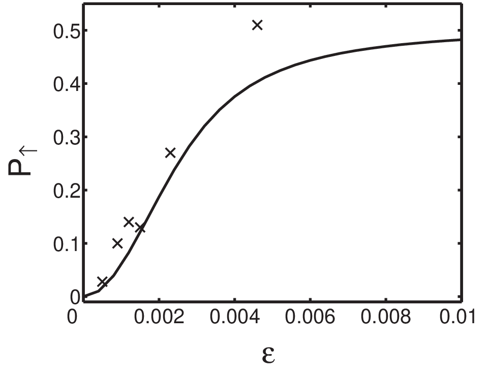
The interpretation for the large detuning (small perturbation) regime, where , was given above. For an intermediate detuning, a small but significant coupling to other () vibrational levels exists. When atoms are transferred from to by the microwave field, a parametric excitation of the atomic wavepacket is induced, thereby exciting “breathing” modes. However, the change in the optical potential also changes the gravitational sag, and hence excites “sloshing” modes along the vertical axis. A wavefunction parametrically excited in an harmonic oscillator will revive after (for ) yielding . A sloshing mode will revive after [64, 66, 67]. These revivals are seen in the middle curve of figure 16 as a partial revival in the echo signal at and a stronger one at , exactly equal to the measured trap oscillation frequency in the radial direction. For the upper curve in figure 16, a faster initial decay of the echo coherence is seen, as expected for a stronger perturbation, followed by a clear revival at . The origin of these revivals is verified in numerical calculations of the echo signal for typical single states in a 2D harmonic oscillator with gravity, having the same oscillation frequency as our experimental data (see figure 17). A similar calculation shows that without the effect of gravity, the revival at is complete. The lack of a perfect revival at in figure 16, is due to the anharmonicity of the Gaussian trap. Note, that our technique is sensitive enough to map the quantum dynamics of a system, due to a perturbation approximately three orders of magnitude smaller than .
For a sufficiently long time the wave packet oscillations of figure 16 damp due to a complete dephasing of the dynamics. At such a long time a simple expression for the echo signal can be given. In particular, assuming random phases between all vibrational states yields the simple relation
| (65) |
Substituting this into equation 64 and averaging over the ensemble yields the expected long-time echo signal. We performed this calculation numerically for a 2D harmonic trap, in gravity, with our measured oscillation frequency and a thermal ensemble with a temperature of clipped at our trap depth of 1.5. The results are shown in figure 18, together with the measured long-time echo signals as a function of perturbation strength11 1 The ensemble average for the clipped thermal distribution in the harmonic trap was calculated as: where are eigenfunction of the harmonic oscillator associated with the horizontal motion and , are associated with (the spring constant is slightly stronger). and are associated with the vertical motion where there is both a change in spring constant and a change in zero point due to different gravitational sag. The sum is over the 3 states for which .. As seen, the calculation for the harmonic trap and the data points for the Gaussian trap show the same qualitative behavior, of improved long time echo when becomes small.
We end this section with a brief discussion of the validity of the “no mixing” condition in our experimental system. We start by noting that typically states of our Gaussian optical trap are thermally populated (this is easily estimated by noting that we typically trap atoms at the standard phase space density provided by laser cooling techniques, ). However, since the duration of the experiment is often much shorter than the longitudinal oscillation time of atoms in our trap, this longitudinal motion is essentially frozen, and we can consider only the thermally populated transverse vibration states. Perturbation theory indicates that a necessary condition for substantial mixing of states is that the energy shift of populated states is comparable to the energy spacing between adjacent states. This means that for thermally populated states the relative energy shift needs to be much smaller than to ensure the “no mixing” condition. In our experiments we typically observe mixing (i.e. a fast decay of the echo coherence) only for much larger relative perturbations of . The solution for this “paradox” is that state mixing by a perturbation can be drastically suppressed by strong selection rules, making the sufficient condition for mixing times larger than the necessary one. For our Gaussian trap such selection rules are provided by the fact that the transverse motion of the atoms is completely separable into two independent one-dimensional motions, with only one-dimensional states thermally populated in each direction. Orthogonality thus ensures mixing only between motional states in each direction separately, whose nearest-state separation is times larger then for the general two-dimensional states. Such enhancement in the stability of the quantum states against perturbation in our separable system is only one of many similarly dramatic difference of the quantum properties between separable and non-separable dynamical systems. Further discussion of such differences exists in section 13 and in references [44, 45].
12 “Multiple Pulses” Sequence
We turn now to investigate the limitations on the coherence time achieved by the echo scheme. According to the time-independent Hamiltonian of equation 39 the echo scheme is expected to provide a complete cancellation of the dephasing for arbitrarily long times, provided the condition is fulfilled for all thermally populated states. However, in real physical systems this is not the case [68]. Two types of mechanisms cause the echo coherence to decay for long times even when . The first type of mechanisms (which we denote as “dynamical” processes) are time-dependent processes leading to a time-dependent resonance frequency of the two-level system. This will cause the two parts of the wave function generated by the first -pulse to acquire different phases during the two “dark” periods of time , hence causing imperfect interference at the time of the second -pulse. Examples of such mechanisms are fluctuations of the trap depth e.g. due to noise in the trap laser power [68], fluctuations in the bias magnetic field giving rise to a fluctuating second order Zeeman shift, and spontaneous Rayleigh scattering of a photon from the trap laser. Rayleigh scattering of photons does not lead to instantaneous loss of coherence, as does a Raman scattering event [10]. Nevertheless, the recoil energy acquired by the atom can significantly change its vibrational level, and therefore its resonance frequency. The result is, again, a time-dependent resonance frequency of the two level systems. Other heating mechanisms, such as pointing instability of the trap laser beam, typically involve a much smaller energy change than Rayleigh photon scattering, hence they induce a much longer time scale for dephasing. The second type of mechanisms for decay of echo coherence ( processes) relates to the finite lifetime of the internal states of the atoms, which is limited mainly by transitions induced by the trap laser light.

As stated above, dynamical processes do not cause instantaneous decoherence, but are characterized by a typical time scale over which a substantial phase difference evolves. If the time between pulses is larger than this time scale, we expect the coherent signal to disappear. The time can be reduced by adding more (equally spaced in time) -pulses between the two -pulses (see figure 19). If the decay of the echo coherence is dominated by dynamical processes, and the time scale for variations in the resonance frequency is longer than , we expect a coherent signal to reappear [69]. The method has a strong similarity with the “decoupling” method used in quantum information schemes in NMR, where a repeated fast refocusing completely stops the dynamics (See reference [70] and references therein).
In this experiment the dipole trap consists of a linearly polarized horizontal Gaussian laser beam focused to a 1/e2 radius of and with a wavelength of , yielding a trap depth of . The transverse oscillation time of atoms in the trap is measured by parametric excitation spectroscopy to be [71] ensuring , for all thermally populated transverse vibrational states. The bias magnetic field is stronger () and turned on after the atoms are loaded into the trap.

As seen in figure 20, the echo signal starts from (indicating perfect coherence) and monotonically approaches (indicating complete loss of coherence). The () coherence time is seen to be . This coherence time is already times longer than the Ramsey fringes decay time, showing the strong suppression of dephasing provided by the echo technique 88 8 The trap in the experiment reported here is 4.5 times deeper than the trap used in section 10, hence the echo coherence time is shorter. The Ramsey decoherence time, which is determined mainly by the temperature of the atoms, is almost equal.. Next, we add more -pulses using the pulse sequence shown in figure 19. First a -pulse creates a coherent superposition state of and . After time the first -pulse is applied, followed by the rest of the -pulses at time intervals . A second -pulse is applied at time after the last -pulse, and followed immediately by an additional -pulse (not shown in the figure) in order to have for a coherent signal for the even number of -pulses that we use. The signal as a function of the total time between the first and the last pulse, , for a pulse sequence containing six -pulses is also shown in figure 20. As seen in the graph, at long times exceeds 1/2, which corresponds to total decoherence for a purely 2-level system. We attribute this to a weak population mixing between -states within the same -manifold as a consequence of spontaneous Raman scattering and off-resonant stimulated Raman transitions involving two photons from the trap laser. The net effect of these transitions is to increase the population of the manifold after the subsequent microwave pulses. To isolate and directly measure this population mixing effect, we measure the population of as a function of time between two population-inverting -pulses 99 9 To further support our interpretation, we verify that a reduction in the transition rate for larger values of the bias magnetic field is observed. Moreover, we verify that the asymptotic slope of the multiple- echo signal is indeed half the slope of the - measurement, as expected from the fact that the population difference of the former is roughly half that of the latter.. From the results, also presented in figure 20, we measure the -conserving transition rate to be . Combining these results with the (independently measured) rate of -changing transitions [10, 29], yields a population decay rate of for the =0 states.
Since the value of at long times is greater than 1/2 we conservatively define the coherence time as the time between the two -pulses where reaches a value of . It is seen that , clearly showing that the additional -pulses substantially increase the coherence time.

As shown in figure 20, the multiple- sequence suffers from an initial small and rapid partial loss of coherence. This is because is not strictly a delta function, hence when more -pulses are added, the mixing to other vibrational levels is increased and the dynamic effects discussed in section 11 appear (The asymptotic value of due to this mixing effect is where is the number of -pulses. The effect is too weak to be observed for ). Shown in the inset of figure 20, is the short time coherence signal for a sequence with 10 -pulses. Wave packet revivals appear for 7 and 14 ms (i.e. a time between -pulses of 0.7 and 1.4 ms) as expected for an harmonic trap with our measured transverse oscillation time of 1.4 ms.
In figure 21 the coherence time is shown as a function of the number of -pulses. It is seen that the coherence time initially shows linear dependence on the number of -pulses and then reaches a maximum value of , a 2.5 fold improvement as compared to the simple echo coherence time. The maximum coherence time is given by a trade-off between suppressing the dephasing due to processes, by adding more -pulses, and the increased dephasing due to mixing to other vibrational states, that the additional -pulses induce.
The decay rate after the initial fast decay shows the residual decoherence, not suppressed by the multiple- scheme. We fit the slope of the intermediate, nearly linear section of the coherence decay curves with a straight line, and correct for the long time slope (We show in figure 21 twice the slope since the decay of coherence contributes only 1/2 to ). We see that the addition of -pulses improves the intermediate slope by a factor of 6. However, as explained before, the initial mixing to other vibrational levels prevents us from fully exploiting this improvement.
13 Quantum Dynamics and Chaos
The coherence properties of trapped atoms are related to their dynamics in the trapping potential. Loosely speaking, the fact that the same electron which is probed by the spectroscopy is used for the trapping, means that there is an inherent interplay between dynamics and spectroscopy. Already at the first demonstration of hyperfine spectroscopy in a dark optical trap [11], it was conjectured that dynamics and spectroscopy are coupled in dipole traps, and that the classical trajectories of the atoms in the trap affect the coherence time of a spectroscopic measurement performed on them. This interplay between dynamics and spectroscopy means that precision spectroscopy in optical traps can serve also as a sensitive probe of the dynamics.
The quantum manifestations of different types of classical dynamics is still an issue of unsettled debates, since the unitary evolution characteristic of quantum mechanics, is inconsistent with the classical definition of chaos, i.e. an exponential sensitivity to the initial conditions. A widely accepted signature of quantum chaos is the correspondence between the spectral statistics of quantized classically chaotic systems and the one of the canonical ensembles of random matrix theory [72]. An alternative approach is to look at the stability of the dynamics with respect to small changes in the Hamiltonian, as first proposed by Peres [46]. In this framework, the “fidelity” denotes the overlap between a state evolved by a Hamiltonian with the same state evolved by a slightly perturbed Hamiltonian [46]. Despite the renewed theoretical and numerical interest in the fidelity and its properties (see references [49, 50, 51, 52, 53, 54, 55, 56, 57, 58, 59]), experimental studies in chaotic and mixed systems are still lacking, mostly due to the difficulty of preparing highly-excited pure quantum states. The use of “echo spectroscopy” eliminates the need for pure quantum state preparation, since quantum fidelities can be experimentally observed even in a thermal ensemble and for extremely highly excited quantum states.
As a specific example, we use in reference [65] “echo spectroscopy” to experimentally measure quantum dynamics of ultra cold 85Rb atoms trapped in atom-optics billiards [73, 74, 75, 76], with underlying chaotic or mixed classical dynamics. In this experiment the trap is a light-sheet wedge billiard, made from two crossed blue detuned light sheets defining the billiard walls and where gravity confines the atoms in the vertical direction [11]. The light sheets have in-focus () dimensions of , and by the use of cylindrical lenses mounted on rotational stages, the wedge angle are adjusted in order to control the classical dynamics1010 10 The structure of phase space in an ideal wedge billiard can be tuned from stability to chaos by varying the vertex half-angle, [77]. For phase space is mixed, and the size of the stable islands oscillates as a function of , a behavior dubbed “breathing chaos”. For the system is fully chaotic.. The confinement in the longitudinal direction is provided by the diffraction of the beams. The very elongated shape of the trap allows us to consider only the transverse motion and neglect the longitudinal one, which has a timescale much longer than the experiment time. The temperature of the atoms is much larger than the mean level spacing in the trap, and the atoms typically occupy many (up to ) states in the trap. The measured echo signal is the ensemble average of all of them.
As shown in reference [44], the echo amplitude can be expressed as a function of the local density of states (LDOS). The LDOS denotes the local average of the absolute-value-squared matrix elements of the transformation matrix from eigenstates of to eigenstates of . Formally, it is simply as a function of averaged over a ensemble of neighboring with approximately the same energy. The width over which the LDOS is nonvanishing is denoted the “bandwidth”, and if it is large, we expect a rapid decay of the echo coherence. In the perturbative regime the LDOS displays system specific features, despite the fact that the underlying classical dynamics is chaotic. In particular, it is evident from the semiclassical calculations of [43, 44] that for atom optics billiards, where the inherent perturbation is localized on the billiard walls, the LDOS has pronounced peaks for corresponding to , where is the typical time between encounters with the wall ( ms in our experiments). This means that the echo signal will show partial revivals for [44].
In figure 22, the decay of the echo signal for different perturbations is presented for a wedge with vertex half-angle (see inset) where the dynamics is fully chaotic. For small perturbations a nonmonotonic decay is seen with a partial revival of correlations for as predicted in [44]. The revivals are seen despite the fact that due to the “high” temperature a large band of energies is occupied in the trap. Partial revivals of correlations in traps where the dynamics is separable are generally expected at time scales equivalent to the 1D level spacing, but their surprising observation here, for a trap with chaotic motion, demonstrates that they are a far more widespread phenomena.

For larger perturbations a crossover to a regime where the decay is monotonic is observed. In this regime the decay is independent of perturbation strength. The perturbation is large enough so the overlap of equivalent eigenstates is small, and this indicates that the effects of quantization of the trap levels should not play a role and a classical description might be possible. Since the echo amplitude can be viewed as a propagator [44], and in our system the thermal de-Broglie wavelength is much smaller than the billiard’s dimensions, it is possible to use a semiclassical propagator [72]. It is then seen that the classical trajectories contributing to the ensemble average of the echo amplitude, are those that after evolving forward in time in and , and then backwards in time in and , return to the vicinity of their initial position. These trajectories we divide into two types: those that during this propagation hit the wall, and those that do not. Since and are highly different mainly in the vicinity of the wall, then the action integral along the first type of trajectories will yield a very large phase and the contribution from these trajectories to the ensemble average of the echo amplitude will average out. However since the second type of trajectories does not feel the difference between the potentials it will retrace its forward propagation backwards in time causing the action integral to vanish. These trajectories will give a perfect contribution. Therefore the echo amplitude in this regime simply measures the classical probability that the particles have not yet hit the wall. Calculations of the echo signal using this model yields good agreement with the experimental measurements.
14 Summary
In this tutorial we present our experiments on the microwave spectroscopy of the ground state hyperfine splitting of optically trapped atoms. We introduce a number of schemes to overcome the inherent perturbation of the atomic levels by the trapping potential.
First, we present a simple, classical model and use it to analyze the light-induced perturbations on optically trapped atoms, and in particular the inhomogeneous broadening of the hyperfine splitting, for a number of trap geometries. An “optimal” trap, achieved by minimizing the surface to volume ratio of the trap (to almost that of a sphere) and by choosing the minimal wall thickness which is allowed by diffraction, is shown to allow an atomic coherence time which is longer than existing single-beam dark traps, and times longer than red-detuned traps.
Next, we demonstrate a scheme for eliminating the trap-induced inhomogeneous broadening of the transition, by adding a weak “compensating” laser, spatially mode-matched with the trapping laser and with a proper detuning and intensity. Despite being tuned close to resonance, this laser induces a negligible change in the dipole potential, and does not considerably increase the spontaneous scattering rate. With the suppression of inhomogeneous broadening, the atomic coherence time is now limited by the much smaller spontaneous scattering time. Whereas in a conventional optical trap the ac Stark shift of the line center strongly depends on the temperature of the atoms, which may drift considerably, in the compensated trap the suppression of the line shift is equally effective for all temperatures. Hence, it provides a means of achieving a higher stability of the line center than that achieved by simply stabilizing the trapping laser detuning and intensity. For relative spectroscopic measurements, such as the proposed measurement of the electron’s permanent electric dipole moment (EDM) [78], only stability (and not absolute accuracy) of the line center is of importance. For example, for a 10 K deep YAG-laser trap, and a compensating beam with a (time averaged) frequency stability, locking the relative intensity between both beams to a stability, will result in stability of the microwave line center.
Conversely, we present a method in which a long microwave pulse is used to select a narrow energy band from the atomic ensemble, around any central energy. The rest of the atoms are expelled from the trap using an on-resonant laser, without perturbing the selected atoms. With our method, the central energy can be chosen to maximize the number of selected atoms by selecting the energy with the highest density of populated states.
We also demonstrate that a macroscopic coherence, lost as a consequence of dephasing of the different populated vibrational levels, can be efficiently revived by stimulating an echo if the trap detuning is large enough so for all thermally populated states. This suppression of dephasing due to perturbations induced by the trap yields a dramatic increase in the coherence time for trapped atoms, that may find important applications for precision spectroscopy and quantum information processing. We further demonstrate that echo spectroscopy can be used to experimentally map the quantum dynamics of trapped atoms, showing a crossover between quantum and classical regimes. In this way it can serve as an extremely sensitive experimental tool for investigating quantum chaos in atom-optics billiards even when more than 106 states are thermally populated, thereby avoiding the need of preparing highly excited pure quantum states.
We demonstrate that the dephasing in microwave spectroscopy of optical trapped atoms due dynamical changes in the trap parameters, or other similar processes, can be suppressed beyond the suppression offered by the simple echo, by using an improved pulse sequence containing additional -pulses. The achieved coherence time is limited by increased mixing between transverse states and, to a lesser extent, the lifetime of the internal states of the atoms. Both these factors are expected to be substantially smaller for a trap laser with much larger detuning, such as in [68]. The demonstrated pulse sequence may also find use in precision spectroscopy of a periodic effect, where the -pulses can be synchronized with the period of that effect.
Finally, we show that “echo spectroscopy” can serve as an important tool for the study of the properties of the fidelity (or Loschmidt Echo) and its relation to the underlying classical dynamics of a quantum system. The main difficulty in experimental studies of these matters, is the preparation of highly-excited pure quantum states. This difficulty can be tackled by using echo spectroscopy, which eliminates the need for pure quantum state preparation and allows the experimental observation of quantum fidelities even in a thermal ensemble and for extremely highly excited quantum states.
A first work in this direction in our experimental system was done in references [44, 45]. Using a perturbative treatment we show that the coherence of the echo scheme is a function of the survival probability or fidelity of eigenstates of the atoms in the trap [44]. The echo coherence and the survival probability display “system specific” features, even when the underlying classical dynamics is chaotic. We performed echo spectroscopy in chaotic and mixed atom-optics billiards, as a function of the perturbation strength, and observed two different regimes [45]. First, a perturbative regime in which the decay of echo coherence is non-monotonic and partial revivals of coherence are observed, as opposed to the prediction from random matrix theory. These revivals are more pronounced in traps with mixed dynamics as compared to traps where the dynamics is fully chaotic. Next, for stronger perturbations, the decay becomes monotonic and independent of the strength of the perturbation. In this regime no clear distinction can be made between chaotic traps and traps with mixed dynamics.
Some of the ideas presented here, have been found useful by other experimental groups. A “compensating” technique has been used [79] to compensate the Stark shift in an ion trap quantum processor. Recently, two other groups working on quantum information processing with single ions and atoms have reported the use of coherence echoes [80, 68].
The combined possibilities offered by our experimental system (control of dynamical phase-space and spectroscopy) can have impact on other fields of study: First, the effect of interactions between the particles trapped in a billiard is an interesting question in the context of semiconductor quantum dots. In atom-optic billiards, the interactions can be tuned in a controlled way, by changing the density of the trapped atoms or by the use of a magnetic field near a Feschbach resonance to change the atom’s scattering length [81]. Next, open systems, which are characterized by a scattering matrix (and not by eigenstates) can be investigated, and related to results in quantum dots, such as universal conductance fluctuations [82]. Finally, chaotic atom-optic billiards, which their unique ability to move from the quantum to the classical regime, can be used for experimental studies of parametrically-dependent Hamiltonians [83] and driven quantum systems [84].
The work described in this tutorial was supported in part by the Israel Science Foundation and the Minerva Foundation.
References
- [1] C. Cohen-Tannoudji. Manipulating atoms with photons. Rev. Mod. Phys., 70:707, 1998.
- [2] W. D. Phillips. Laser cooling and trapping of neutral atoms. Rev. Mod. Phys., 70:721, 1998.
- [3] S. Chu. The manipulation of neutral particles. Rev. Mod. Phys., 70:685, 1998.
- [4] N. Ramsey. Experiments with separated oscillatory fields and hydrogen masers. Rev. Mod. Phys., 62:541, 1990.
- [5] J. R. Zacharias. Unpublished, as described in Ref. [4].
- [6] M. A. Kasevich, E. Riis, and S. Chu. rf spectroscopy in an atomic fountain. Phys. Rev. Lett., 63:612, 1989.
- [7] E. L. Raab, M. Prentiss, A. Cable, S. Chu, and D. E. Pritchard. Trapping of neutral sodium atoms with radiation pressure. Phys. Rev. Lett., 59:2631, 1987.
- [8] S. Chu, J. E. Bjorkholm, A. Ashkin, and A. Cable. Experimental observation of optically trapped atoms. Phys. Rev. Lett., 57:314, 1986.
- [9] R. Grimm, M. Weidemuller, and Y. B. Ovchinnikov. Optical dipole traps for neutral atoms. Adv. At. Mol. Opt. Phy., 42:95, 2000.
- [10] R. A. Cline, J. D. Miller, M. R. Matthews, and D. J. Heinzen. Spin relaxation of optically trapped atoms by light scattering. Opt. Lett., 19:207, 1994.
- [11] N. Davidson, H. J. Lee, C. S. Adams, M. Kasevich, and S. Chu. Long atomic coherence times in an optical dipole trap. Phys. Rev. Lett., 74:1311, 1995.
- [12] C. S. Adams, H. J. Lee, N. Davidson, M. Kasevich, and S. Chu. Evaporative cooling in a crossed dipole trap. Phys. Rev. Lett., 74:3577, 1995.
- [13] J. D. Miller, R. A. Cline, and D. J. Heinzen. Far-off-resonance optical trapping of atoms. Phys. Rev. A, 47:R4567, 1993.
- [14] T. Takekoshi and R. J. Knize. CO2 laser trap for cesium atoms. Opt. Lett., 21:77, 1996.
- [15] N. Friedman, A. Kaplan, and N. Davidson. Dark optical traps for cold atoms. Adv. At. Mol. Opt. Phys., 48:99, 2002.
- [16] C. Cohen-Tannoudji. Atomic motion in laser light. In J. Dalibard, J.-M. Raimond, and J. Zinn-Justin, editors, Fundamental systems in quantum optics, page 1, Amsterdam, The Netherlands, 1990. Elsevier Science Publishers.
- [17] W. D. Phillips. Laser cooling, optical traps and optical molasses. In J. Dalibard, J.-M. Raimond, and J. Zinn-Justin, editors, Fundamental systems in quantum optics, page 165, Amsterdam, The Netherlands, 1990. Elsevier Science Publishers.
- [18] C. S. Adams and E. Riis. Laser cooling and trapping of neutral atoms. Prog. Quant. Electron., 21:1, 1997.
- [19] C. Cohen-Tannoudji, J. Dupont-Roc, and G. Grynberg. Atom-photon interactions. John Wiley & Sons, inc., New York, 1992.
- [20] V.S. Letokhov. Narrowing of the doppler width in a standing light wave. JETP Lett., 7:272, 1968.
- [21] A. Ashkin. Acceleration and trapping of particles by radiation pressure. Phys. Rev. Lett., 24:156, 1970.
- [22] T. Takekoshi, J. R. Yeh, and R. J. Knize. Quasi-electrostatic trap for neutral atoms. Opt. Comm., 114:421, 1995.
- [23] M. D. Barrett, J. A. Sauer, and M. S. Chapman. All-optical formation of an atomic Bose-Einstein condensate. Phys. Rev. Lett., 87:010404, 2001.
- [24] H. J. Lee, C. S. Adams, M. Kasevich, and S. Chu. Raman cooling of atoms in an optical dipole trap. Phys. Rev. Lett., 76:2658, 1996.
- [25] Yu. B. Ovchinnikov, I. Manek, A. I. Sidorov, G. Wasik, and R. Grimm. Gravito-optical atom trap based on a conical hollow beam. Europhys. Lett., 43:510, 1998.
- [26] T. Kuga, Y. Torii, N. Shiokawa, and T. Hirano. Novel optical trap of atoms with a doughnut beam. Phys. Rev. Lett., 78:4713, 1997.
- [27] R. Piestun and J. Shamir. Control of wave-front propagation with diffractive elements. Opt. Lett., 19:771, 1994.
- [28] G. Shabtay, Z. Zalevsky, U. Levy, and D. Mendlovic. Optimal synthesis of three-dimensional complex amplitude distributions. Opt. Lett., 25:363, 2000.
- [29] R. Ozeri, L. Khaykovich, and N. Davidson. Long spin relaxation times in a single-beam blue-detuned optical trap. Phys. Rev. A, 59:R1750, 1999.
- [30] R. Ozeri, L. Khaykovich, N. Friedman, and N. Davidson. Large-volume single-beam dark optical trap for atoms using binary phase elements. J. Opt. Soc. Am. B, 17:1113, 2000.
- [31] A. Kaplan, N. Friedman, and N. Davidson. Optimized single-beam dark optical trap. J. Opt. Soc. Am. B, 19:1233, 2002.
- [32] L. Cacciapuoti, M. de Angelis, G. Pierattini, and G.M. Tino. Single-beam optical bottle for cold atoms using a conical lens. Eur. Phys. J. D., 14:373, 2001.
- [33] S. Kulin, S. Aubin, S. Christe, B. Peker, S. L. Rolston, and L. A. Orozco. A single hollow-beam optical trap for cold atoms. J. Opt. B: Quantum Semiclass. Opt., 3:353, 2001.
- [34] N. Friedman, L. Khaykovich, R. Ozeri, and N. Davidson. Compression of cold atoms to very high densities in a rotating-beam blue-detuned optical trap. Phys. Rev. A, 61:031403(R), 2000.
- [35] I. H. and P. S. Jessen. Quantum-state control in optical lattices. Phys. Rev. A, 57:1972, 1998.
- [36] J. Dalibard and C. Cohen-Tannouji. Laser cooling below the Doppler limit by polarization gradients: simple theoretical models. J. Opt. Soc. Am. B, 6:2023, 1989.
- [37] L. Khaykovich, N. Friedman, S. Baluschev, D. Fathi, and N. Davidson. Ultrasensitive two-photon spectroscopy based on long spin-relaxation time in a dark optical trap. Europhys. Lett., 50:454, 2000.
- [38] S. J. M. Kuppens, K. L. Corwin, K. W. Miller, T. E. Chupp, and C. E. Wieman. Loading an optical dipole trap. Phys. Rev. A, 62:013406, 2000.
- [39] A. Kaplan, M. Andersen, and N. Davidson. Suppression of inhomogeneous broadening in rf spectroscopy of optically trapped atoms. Phys. Rev. A, 66:045401, 2002.
- [40] H. Katori, T. Ido, and M. Kuwata-Gonokami. Optimal design of dipole potentials for efficient loading of Sr atoms. J. Phys. Soc. Jap., 68:2479, 1999.
- [41] H. Katori and M. Takamoto. Ultrastable optical clock with neutral atoms in an engineered light shift trap. Phys. Rev. Lett., 91:173005, 2003.
- [42] M. Takamoto and H. Katori. Spectroscopy of the clock transition of 87Sr in an optical lattice. Phys. Rev. Lett., 91:223001, 2003.
- [43] D. Cohen and T. Kottos. Parametric dependent Hamiltonians, wave functions, random matrix theory, and quantal-classical correspondence. Phys. Rev. E, 63:036203, 2001.
- [44] M. F. Andersen, T. Grunzweig, A. Kaplan, and N. Davidson. Revivals of coherence in chaotic atom-optics billiards. Phys. Rev. A, 69:063413, 2004.
- [45] M. F. Andersen, A. Kaplan, T. Grunzweig, and N. Davidson. Decay of Quantum Correlations in Atom Optics Billiards with Chaotic and Mixed Dynamics, 2004. quant-ph/0404118.
- [46] A. Peres. Stability of quantum motion in chaotic and regular systems. Phys. Rev. A, 30:1610, 1984.
- [47] H. G. Schuster. Deterministic Chaos. Physik-Verlag, Weinheim, Germany, 1984.
- [48] R. A. Jalabert and H. M. Pastawski. Environment-independent decoherence rate in classically chaotic systems. Phys. Rev. Lett., 86:2490, 2001.
- [49] F. M. Cucchietti, H. M. Pastawski, and R. Jalabert. Dynamical origin of decoherence in classically chaotic systems. Physica A, 283:285, 2000.
- [50] Ph. Jacquod, P. G. Silvestrov, and C. W. J. Beenakker. Golden rule decay versus Lyapunov decay of the quantum Loschmidt echo. Phys. Rev. E, 64:055203, 2001.
- [51] N. R. Cerruti and S. Tomsovic. Sensitivity of wave field evolution and manifold stability in chaotic systems. Phys. Rev. Lett., 88:054103, 2002.
- [52] F. M. Cucchietti, H. M. Pastawski, and D. A. Wisniacki. Decoherence as decay of the Loschmidt echo in a Lorentz gas. Phys. Rev. E, 65:045206(R), 2002.
- [53] F. M. Cucchietti, C. H. Lewenkopf, E. R. Mucciolo, H. M. Pastawski, and R. O. Vallejos. Measuring the Lyapunov exponent using quantum mechanics. Phys. Rev. E, 65:046209, 2002.
- [54] T. Prosen. General relation between quantum ergodicity and fidelity of quantum dynamics. Phys. Rev. E, 65:036208, 2002.
- [55] J. Emerson, Y. S. Weinstein, S. Lloyd, and D. G. Cory. Fidelity decay as an efficient indicator of quantum chaos. Phys. Rev. Lett., 89:284102, 2002.
- [56] J. Vanicek and E. J. Heller. Semiclassical evaluation of fidelity in the Fermi-golden-rule and Lyapunov regimes. Phys. Rev. E, 68:056208, 2003.
- [57] D. A. Wisniacki. Short time decay of the Loschmidt echo. Phys. Rev. E, 67:016205, 2002.
- [58] G. Benenti, G. Casati, and G. Veble. Asymptotic decay of the classical Loschmidt echo in chaotic systems. Phys. Rev. E, 68:036212, 2003.
- [59] M. Hiller, T. Kottos, D. Cohen, and T. Geisel. Quantum reversibility: Is there an echo? Phys. Rev. Lett., 92:010402, 2004.
- [60] M. Nielsen and I. L. Chuang. Quantum Information and Quantum Computation. Cambridge University Press, 2001.
- [61] E. L. Hahn. Spin echoes. Phys. Rev., 80:580, 1950.
- [62] N. A. Kurnit, I. D. Abella, and S. R. Hartmann. Observation of a photon echo. Phys. Rev. Lett., 13:567, 1964.
- [63] L. Allen and J. H. Eberly. Optical Resonance and Two-Level Atoms. Dover Publications, Inc., New York, 1987.
- [64] F. B. J. Buchkremer, R. Bumke, H. Levsen, G. Birkl, and W. Ertmer. Wave packet echoes in the motion of trapped atoms. Phys. Rev. Lett., 85:3121, 2000.
- [65] M. F. Andersen, A. Kaplan, and N. Davidson. Echo spectroscopy and quantum stability of trapped atoms. Phys. Rev. Lett., 90:023001, 2003.
- [66] R. Ejnisman, P. Rudy, H. Pu, and N. P. Bigelow. Revivals, damping, and coherence times of atomic wave packets in optical lattices. Phys. Rev. A, 56:4331, 1997.
- [67] G. Raithel, W. D. Phillips, and S. L. Rolston. Collapse and revivals of wave packets in optical lattices. Phys. Rev. Lett., 81:3615, 1998.
- [68] S. Kuhr, W. Alt, D. Schrader, I. Dotsenko, Y. Miroshnychenko, W. Rosenfeld, M. Khudaverdyan, V. Gomer, A. Rauschenbeutel, and D. Meschede. Coherence properties and quantum state transportation in an optical conveyor belt. Phys. Rev. Lett., 91:213002, 2003.
- [69] M. F. Andersen, A. Kaplan, T. Grunzweig, and N. Davidson. Suppression of dephasing of optically trapped atoms. Phys. Rev. A, 70:013405, 2004.
- [70] N. A. Gershenfeld and I. L. Chuang. Bulk spin-resonance quantum computation. Science, 275:350, 1997.
- [71] S. Friebel, C. DAndrea, J. Walz, M. Weitz, , and T. W. Hansch. Co2-laser optical lattice with cold rubidium atoms. Phys. Rev. A, 57:R20, 1998.
- [72] M. C. Gutzwiller. Chaos in Classical and Quantum Mechanics. Springer-Verlag, New York, 1990.
- [73] V. Milner, J. L. Hanssen, W. C. Campbell, and M. G. Raizen. Optical billiards for atoms. Phys. Rev. Lett., 86:1514, 2001.
- [74] N. Friedman, A. Kaplan, D. Carasso, and N. Davidson. Observation of chaotic and regular dynamics in atom-optics billiards. Phys. Rev. Lett., 86:1518, 2001.
- [75] A. Kaplan, Nir Friedman, M. Andersen, and N. Davidson. Observation of islands of stability in soft wall atom-optics billiards. Phys. Rev. Lett., 87:274101, 2001.
- [76] M. F. Andersen, A. Kaplan, N. Friedman, and N. Davidson. Stable islands in chaotic atom-optics billiards, caused by curved trajectories. J. Phys. B: At. Mol. Opt. Phys., 35:2183, 2002.
- [77] H. E. Lehtihet and B. N. Miller. Numerical study of a billiard in a gravitational field. Physica D, 20:93, 1986.
- [78] C. Chin, V. Leiber, V. Vuletic, A. J. Kerman, and S. Chu. Measurement of an electron’s electric dipole moment using s atoms trapped in optical lattices. Phys. Rev. A, 63:033401, 2001.
- [79] H. Häffner, S. Gulde, M. Riebe, G. Lancaster, C. Becher, J. Eschner, F. Schmidt-Kaler, and R. Blatt. Precision measurement and compensation of optical stark shifts for an ion-trap quantum processor. Phys. Rev. Lett., 90:143602, 2003.
- [80] M. A. Rowe, A. Ben-Kish, B. DeMarco, D. Leibfried, V. Meyer, J. Beall, J. Britton, J. Hughes, W. M. Itano, B. Jelenkovi, C. Langer, T. Rosenband, , and D. J. Wineland. Transport of quantum states and separation of ions in a dual RF ion trap. Quantum Information and Computation, 2:257, 2002.
- [81] J. M. Vogels, C. C. Tsai, R. S. Freeland, S. J. J. M. F. Kokkelmans, B. J. Verhaar, and D. J. Heinzen. Prediction of Feshbach resonances in collisions of ultracold rubidium atoms. Phys. Rev. A, 56:R1067, 1997.
- [82] H.U. Baranger and R.M. Westervelt. Chaos in ballistic microstructures. In G. Timp, editor, Nanotechnology, chapter 14, page 537. Springer, 1998.
- [83] D. Cohen, A. Barnett, and E. J. Heller. Parametric evolution for a deformed cavity. Phys. Rev. E, 63:046207, 2001.
- [84] D. Cohen and T. Kottos. Quantum-mechanical nonperturbative response of driven chaotic mesoscopic systems. Phys. Rev. Lett., 85:4839, 2000.