Ropelength of tight polygonal knots
Abstract.
A physical interpretation of the rope simulated by the SONO algorithm is presented. Properties of the tight polygonal knots delivered by the algorithm are analyzed. An algorithm for bounding the ropelength of a smooth inscribed knot is shown. Two ways of calculating the ropelength of tight polygonal knots are compared. An analytical calculation performed for a model knot shows that an appropriately weighted average should provide a good estimation of the minimum ropelength for relatively small numbers of edges.
1. Introduction
Knots tied on material objects, e.g. a rope of a finite thickness, are called physical knots [18]. It is well known from everyday life that open knots can be tightened by pulling apart the loose ends of the rope. Tightening a closed knot, i.e. a knot tied on a rope whose ends are spliced, is more difficult since one has to engage processes in which the rope will reduce its length while keeping its diameter intact. Such a process, difficult to create in the laboratory, can be easily simulated numerically and we find in the literature various examples of such simulations [20, 2, 14, 12, 17, 19, 4]. From the intuitive point of view, it is rather obvious that in tightening a knot tied on a rope of a finite diameter, one must arrive at a conformation at which the tightening process stops. This conformation is called tight. Any small change in the shape of a tight conformation needs an elongation of the rope. Obviously, tight conformations of knots tied on different types of rope, with different physical properties, will be different. Thus, to make the notion of the tight knot unambiguous, one must specify the physical model of the rope on which the knot is tied. The simplest of such models is the perfect rope. Perfect rope is perfectly floppy – needs no force to be bent, but, at the same time, it is perfectly hard – needs an infinite force to be squeezed, its diameter always remains intact. It is also perfectly slippery. Its formal definition will be given in the next section.
Tight conformations can be seen as minimizers of the ropelength function [1, 11]. The minima can be only local. While it has been shown that global minima exist [3, 7], with the exception of the trivial knot and some simple links, the minimizing conformations are not known. Knots in the conformations at which the ropelength reaches its global minimum are called ideal. As long as the ideal conformations are not known analytically, we cannot be certain that the conformation at which one arrives is ideal.
In all simulations of the processes in which knots are tightened, the knots are represented by a finite sequence of points in space. When connected, the points can be seen as vertices of a self-avoiding polygon. Most often the simulation programs either start from a non-equilateral conformation and aim at making it equilateral (e.g. SONO) or start from an equilateral conformation and try to keep it such (crankshaft rotations). Let be such an equilateral polygon. The essential problem we face is to construct, using the coordinates of the vertices of , a smooth knot which can be seen as the axis of the knot tied on the perfect rope. In constructing , we make some assumptions concerning the shape of the pieces of which it is built. In what follows we assume that the knot is built from smoothly connected arcs inscribed into , which makes the knot smooth. As a result of this assumption and provided the radius of the rope is properly chosen, we show that the knot can indeed be tied with perfect rope leaving it self-avoiding. On the other hand, we also know that the inscribed knot is not ideal, thus, its ropelength can serve only as an upper bound for the minimum ropelength of the unknown ideal conformation. In finding tight polygonal knots with an increasing number of vertices, we see that the ropelength of the inscribed smooth knots converges to a value, which we believe is the ropelength of the ideal conformation, although we will not prove that here. This convergence is slow however, and one might want an approximation using relatively few edges. This is especially important for complicated knots where the number of edges needed to adequately approximate the smooth ropelength would not be practical. With this aim, a second, weighted-average, approach is explored. This technique provides surprisingly accurate approximations with relatively few edges. Together, we provide both a theoretically-sound approach with slow convergence and a practical approach with fast convergence. Depending on the application, we expect that both techniques will be useful.
2. Computing upper bounds for smooth knots inscribed in tight polygons
2.1. Ropelength of knots tied on the perfect rope
Smooth ropelength models perfect rope as a non self-intersecting tube with a knot as its core. For completeness, we include these definitions and some properties of this knot energy.
Definition 1.
For a knot and , let be the disk of radius centered at lying in the plane normal to the tangent vector at . Let
The quantity is called the thickness radius of . Define the ropelength of to be
where is the arclength of .
The thickness radius is the radius of a thickest tube that can be placed about the knotted core without self-intersection. Note that in some of the literature, the thickness refers to the diameter of this thickest tube, in which case the ropelength is half of what we use here. The problem we face is how, knowing the shape of , to find .
Suppose we are given a concrete knot and we are trying to reproduce it with an impenetrable tube. Thus, serves here as the core of the knotted tube. We have to pay attention to two types of interactions between the tube’s normal disks that restrict the radius of the tube.
- (A)
The interactions between the discs centered on pairs of points located infinitesimally close to the diagonal of – these normal disks will start overlapping when the curvature radius is smaller than .
- (B)
The interactions between the discs centered on points located away from the diagonal of – the disks will start overlap when the Euclidean distance between the points is smaller than .
Figure 1 illustrates the problem. These intuitive observations are captured by the quantities below and the subsequent lemma.

Definition 2.
For a knot with unit tangent map , let be the minimum of the radius of curvature measured at each of the points on the knot. The doubly-critical self-distance is the minimum distance between pairs of points on the knot whose chord is perpendicular to the tangent vectors at the both of the points. In other words, let
where is the chord connecting and . Define the doubly-critical self-distance by
where is the standard norm.
There is a fundamental relationship between , , and .
Lemma 3.
Suppose is a knot. Then
Proof.
See [11]. ∎
After reworking the definition of , one can extend Lemma 3 to include (and thus curves). The following is taken from [6]. For a function , define the dilation of by
Note that if is a knot parameterized by arclength with unit tangent map , then . Thus, the dilation gives a generalization for to knots that are . Since and are equal for knots, we use to denote for all knots. If a knot is but not , then , in which case is assumed to be . In this paper, we are mainly interested in knots, in which case is finite and is positive. Alternate, but equivalent, approaches for defining the ropelength of knots are explored in [8, 3].
Lemma 4.
Suppose is a knot. Then
Furthermore, if is , then .
2.2. Ropelength of polygonal knots
As mentioned in the introduction, the problem we face in analyzing knots provided by numerical simulations is that they are not given in a smooth continuous form. For instance, programs based on the SONO algorithm deliver equilateral polygonal knots. Let be such a knot. It is represented by a sequence of points whose positions are indicated by vectors . We shall refer to them as the vertices or beads of the polygonal knot that one obtains by joining consecutive vertices. We define
The vectors will be called edges. When referring to the vertices as points on a polygonal knot, we shall omit the vector notation.
Remark: Because the knots that we are considering are closed, whenever the vertex index happens to be larger than , we assume that . Similarly, when the index happens to be smaller than 1, we assume .
In what follows, we will use the notion of the index distance between the vertices:
Note that alternate approaches have been appeared in [9, 21, 15, 10, 16, 5, 8, 17, 19, 4]. In the SONO simulations, the vertices of a knot interact with each other as if they were spheres, the properties of which will be later. Taking into account the representation, we shall extend the notion of the thickness radius in terms of the virtual spheres. We do this by defining notions of and for polygons similar to the characterization theorem (Lemma 4) for smooth thickness radius.
Definition 5.
Suppose is an equilateral polygonal knot with edge lengths . Let
where is the turning angle of the tangent vectors at . Note that is the radius of an arc of a circle that can be inscribed in the corner at so that intersects both adjacent edges at the midpoint and the tangent at the midpoints coincide with the tangents on at the midpoints. Let
where is the maximum turning angle. See Figure 2.

Definition 6.
Let be a polygonal knot. We define the sphere thickness radius to be
where , the sphere radius, is half the minimum distance between vertices whose index distance is at least .
The construction of the sphere thickness radius needs a few words of explanation. Suppose is an equilateral knot. Imagine that about each of the vertices, there is a sphere of radius . When is larger than , the spheres about nearby vertices intersect. The cases in which need special attention, but since they never occur in the simulations we eventually analyze, we exclude them assuming implicitly in what follows that . The surface of the union of all spheres is bumpy, so we refer to this as the corrugated tube or bead rope about the knot. The problem we face is to inflate the spheres as much as possible without violating the condition of the self-avoidedness of the corrugated tube formed by their union.
First, let us explain what we mean by self-avoiding in the case of the corrugated tube. Consider three consecutive vertices , , and and the spheres , , and , around them all of radius . The spheres and intersect at a circle whose radius equals . The spheres and intersect at a circle of the same radius. Let and be the disks filling the circles. The disks are inclined at an angle equal to the turning angle . We assume that the disks are hard and hence cannot overlap; thus, at most they may become tangent at a single point. The latter happens when the sphere radius . For a given polygonal knot , the smallest of such radii is . When is chosen larger than , we see the behavior shown in Figure 3a.
When , all portions of the corrugated tube are well-defined locally and one must check if index-distant vertices are too Euclidean-close. Let us explain, what we mean by stating that the portions of the corrugated tube are well-defined. Each portion of the corrugated tube is a sphere with two pieces cut off. The cutting planes are perpendicular to the polygon edges and are located at the midpoints. Consecutive portions are thus connected with disks of radius . As stated above, the disks are assumed to be hard and they are not allowed to overlap. A portion of the corrugated tube which fulfills the condition is said to be well-defined. If the Euclidean distance between two vertices is smaller than , the portions of the corrugated tube would overlap. Thus, we check all the Euclidean distances between sufficiently index-distant vertices and find the smallest one. This will be the value of . This is a geometrical interpretation of the self-avoidedness conditions found in the definition of . When is chosen larger then , we see the behavior shown in Figure 3b.

We will be mainly interested in optimizing , but to do so we need a scale-invariant version of . There are various ways to do this and we explore two normalizations in the next section. The corrugation will play a part in how the knot packs efficiently in these optimizing conformations. In the short term, our goal is to show that for a sufficiently “thick” polygon , there exists a smooth knot inscribed in whose thickness radius is close to . We first present the inscribing algorithm. A similar formulation for inscribing polygons appears in [17].
Proposition 7.
For a given -edge equilateral polygonal knot with edge length , a curve can be inscribed in in such a way that . Furthermore, there exists a bijection between and so that for each pair and , we have .
Proof.
An arc of a circle of radius can be inscribed at such that is tangent to and and intersects the adjacent edges at the midpoints. Let be the result of inscribing arcs of radius at each vertex and removing the bypassed corners. Since there is no overlapping of adjacent inscribed arcs, is well-defined as a (possibly self-intersecting) closed curve. The curve has a piece-wise constant radius of curvature, and . The knot is and piecewise , and thus, lies in the category of curves.
For each on the inscribed curve , we define a unique point on . If is a midpoint on , let . Otherwise, lies on an arc, say , whose center is . Let be the intersection of the ray with (see Figure 4). Simple trigonometric calculations show that
∎

For each , we say the corresponding vertex is the vertex which generates the arc on which lies. The midpoint of each edge has two corresponding vertices. It will be convenient to think of the midpoint as corresponding to each vertex in different situations and this will not pose any problems in this work. Note that the smaller is, the closer the inscribed curve will be to the polygon .
The corrugated tube about the polygon is a union of many spheres, some of which are allowed to intersect. The intersection between the surface of two adjacent spheres consists of a circle whose radius is and whose center is the midpoint of the edge. This value will be important, so we define . We will show now that the smooth tube of radius about is non-self intersecting, i.e. that the thickness radius of is at least . See Figure 5. This is a bit delicate and will take some effort to prove. We will need the following technical lemma.

Lemma 8.
Let be an equilateral polygonal knot with edge lengths and and be the smooth knot inscribed in via the algorithm of Proposition 7. If and , then , where and are the vertices corresponding to and .
Proof.
Suppose . Now is the minimum arclength on measured over the two paths connecting and . By the construction of the inscribed smooth knot, we know that is no larger than the arclength along between the corresponding points and . In the worst case, both and are midpoints and their corresponding vertices and lie in the shorter arc between and . In such a case, we have
where denotes the minimum arclength when walking along the polygon . Now where is the number of edges between and . Thus, or . ∎
In other words, if , then we know that the corresponding vertices and will be a part of the set over which is computed. This will be important in ensuring that bounds .
We now have the tools to bound the thickness radius of the inscribed knot .
Theorem 9.
Let be an equilateral polygonal knot with edge lengths and and be the smooth knot inscribed in via the algorithm of Proposition 7. Then .
Proof.
By the construction of , we know that . We split the proof into two cases: when and when .
In the former case, we have .
In the latter case, we assume . By [17], we know that when is realized at a pair of points, say and , then . Therefore, the corresponding vertices and have by Lemma 8. Let and be the disks of radius normal to at and respectively and let and be the spheres of radius centered at and respectively. Now and lie inside and respectively, and by the definition of , we know that the interiors of and do not intersect. Furthermore, the normal disks and are contained within and respectively. Therefore, and can only intersect, in the worst case, on the boundary. This implies that or . ∎
The previous result is not sharp in general. However, for the sake of this paper, it does provide a computable lower bound for the thickness radius of . Furthermore, the length of , which is smaller than the length of , can be computed explicitly. We call the inscribed ropelength and denote it . The value of is an upper bound for the ropelength of the inscribed , and as (note that changing affects , , and ), our bound on approaches . Since , the inscribed arcs lie within the corrugated tube about , which guarantees that has the same knot type as . Since is a smooth knot with the same knot type as , we have a bound on the ropelength of one smooth knot within the knot type. Thus, we have an upper bound for the minimum smooth ropelength for the given knot type.
3. Interpretation of simulations performed with the SONO algorithm
Let us now describe the SONO algorithm using the notions defined above. First notice that in discussing the ropelength of smooth knots, we are considering knots of a given length looking for their thickness radius . The value is the maximum radius for which could be inflated without violating the conditions that the surface of the tube must remain self-avoiding. The value is the ropelength of . The application of the virtual inflation suggests numerical calculations in which the inflation process forces the knot to change its conformation. Such changes may maximize and thus minimize . Working with polygonal knots, it proves more convenient to consider a different scheme in the simulations: keep the sphere radius fixed and shorten the edge length so that the knot eventually arrives at a conformation for which . This is the approach we discuss below.
3.1. Basic procedures of SONO
There are two essential procedures on which SONO is based [13]. The basic goal of SONO is to reduce subject to the constraint that , for some fixed rope radius . In practice, we choose . The reduction of the polygon length is achieved by reducing its edge length . We aim at simulating equilateral knots; thus one of these procedures called EqualizeEdges (EE), checks the length of the edges, and, if they differ from the desired value , introduces necessary corrections. Suppose the distance between vertex and is different from the desired value. Then the vertices are shifted toward new positions so that their distance is closer to :
. Usually we work with .
As a result of multiple applications of the procedure, the dispersion of the edge lengths in the final conformations becomes very small, and thus, we consider the knots we get from our simulations as equilateral.
The second procedure called RemoveOverlaps (RO), checks the distances between the vertices. When the RO procedure finds that the minimum distance is violated, the vertices and are shifted away from each other to a distance equal to or, what proves to speed up the initial stage of the tightening process, exceeding by :
where and is usually set equal to 1/2. The value of changes during the tightening process. Initially it is of the order and reaches the level of at its end.
The procedures RO and EE are in some circumstances contradictory, but their multiple application leads to simultaneous reduction of both the overlaps and the dispersion of the edge lengths. Both parameters are constantly monitored.
When the edge length is small, the tightened polygonal knots develop short regions where tends to become small. An additional procedure ControlCurvature (CC) monitors this, never allowing the external angle between the consecutive edges to be larger than . This, in particular in the final stages of the tightening, makes sure that the tight conformation of will have .
3.2. Physical sense of the SONO algorithm and practical details of simulations
Let us now discuss the physical sense of the simulation based on the SONO algorithm. The simulated knot can be seen as tied on a closed necklace of beads. The necklace is unusual, because its beads are unusual: if their index distance , they are allowed to overlap, otherwise they behave as hard spheres of radius and repel infinitely hard. The RO procedure simulates this interaction. Because of the action of the EE procedure, the centers of the consecutive beads can be seen as connected with nonextensible rods of controlled length . The rods are connected to each other by elasticity free but angle-limiting joints. Each of the beads has the shape of a sphere with two parts of it cut off. The cutting planes are located in the middle of the edges which lead to it. Consecutive beads are thus connected via disks of radius . The necklace can be bent in any direction but only to some extent: the CC procedure limits the angle between the consecutive rods to . As a result, , which prevents the disks separating consecutive beads to overlap. At most they are allowed to become tangent. Because of its construction, the surface of the bead rope is not smooth. It is corrugated and the corrugation is more pronounced, the larger the distance between consecutive beads. This distance is, of course, the edge length .
The tightening process runs as follows. Suppose we start with a loose conformation. The EE and RO procedures make the lengths of all edges equal and remove overlaps between the beads. After multiple applications of the procedures, the dispersion of the edge lengths and the sum of all overlaps fall below a fixed level. Then SONO reduces the required edge length . Now, as the EE procedure tries to adjust the length of the edges to the new value by shortening the distance between consecutive beads, new overlaps may appear. Subsequently they are removed by the RO procedure. And so on.
In the final tight conformation, the dispersion of edge lengths and the sum of all overlaps are smaller than which allows us to consider the closest beads as just touching. Keeping in mind that the CC procedure does not allow to be smaller than , we may consider the final tight knot as a polygonal, equilateral knot whose .
The shrinking rope forces the knot to change its conformation. At the end, we arrive at a conformation for which further shortening is no longer possible because it creates non-removable overlaps. Obviously, if the number of beads is small, the final value of is large and the bead rope is strongly corrugated. This may create problems, since the knot is more likely to become stuck in a local minimum. The reason for this is as follows: one part of the rope winding around another part may get into a groove between consecutive beads even if shifting it to another groove would allow further shortening of the rope. The shifting will not be achieved by SONO, because it would need a (rather large) temporary increase of the ropelength. Working with a small number of beads, we set to a higher value to minimize these effects. In general, the tightening process should be seen as a physical experiment in which the experimenter watches and adjusts the parameters.
3.3. The problem of finding the right ropelength, an experimental approach
In Figure 6, we have the tightest conformations of the trefoil knot found by SONO working with rope consisting of 15, 30, 60, 120, 240, and 480 vertices.

It seems plausible that the best estimation of the minimal length of the rope needed to tie a particular knot will come from analyzing the polygonal conformation obtained for highest . As seen in the figure, at the surface of the bead rope is visually smooth – the corrugation of its surface, so visible at , , , becomes undetectable by the naked eye. The problem we face is that in tightening much larger knots, for instance the torus knot, reaching this level of the surface smoothness would require a very large number of beads, which is both awkward and time-consuming. For practical reasons, it is reasonable to limit the number of beads as much as possible. We present a picture showing the details of the SONO tightened trefoil for such a small in Figure 7.

Calculations run faster when is small, but what about the accuracy of the ropelength we can extract from the analysis of the final, tight conformation?
4. Ropelength of SONO knots
We are mainly interested in understanding the optimal conformations of . However, varies with scale, so one could always increase simply by scaling the polygon. In the second section, we explored one way to normalize , namely by analyzing the ropelength of the inscribed knot . In doing so, we overestimate the minimum ropelength. In this section, we present a different normalization that will underestimate the ropelength. In the next section, we combine these two notions to obtain a reasonable approximation of the minimum ropelength with relatively few edges.
The simplest way to determine the ropelength is to sum the length of all edges of the knot and divide by :
In what follows we shall refer to as the raw polygonal ropelength. In calculating the ropelength in such a simplistic manner, we implicitly assume that the polygonal knot makes the axis of a rope of radius 1, which is obviously wrong. Certainly, if the cylindrical segments of the rope are not to overlap, the radius should be smaller. This becomes clear for large . However erratic the raw polygonal length may seem, it will prove to be very useful.
It is interesting to see how the values of the raw polygonal and inscribed ropelength behave in practice as increases. For the sake of convenience, Figure 8 shows both values plotted versus the edge length .

First notice that as the edge length diminishes, the raw polygonal and the inscribed ropelengths apparently converge to a common value. We call this value the true ropelength, denoted . In spite of its erratic nature, the raw polygonal ropelength converges faster than the inscribed ropelength. The raw polygonal ropelength underestimates while the inscribed ropelength overestimates the ropelength. Can one find a weighted average that will accurately estimate the ropelength with relatively few edges? Below, we present a heuristic reasoning which provides the answer.
4.1. The problem of finding the right ropelength, an analytic approach
By looking at SONO tightened knots, see for instance Figure 9, one may notice that we often deal with pieces of a rope winding around other pieces of the rope. At smaller , the rope is strongly corrugated. Thus, to be precise, we deal with pieces of a corrugated rope winding around other pieces of the corrugated rope. In a model situation shown also in the picture, the central piece is straight and the other piece winds tightly around it. By analyzing the raw polygonal and inscribed ropelength functions in this simplified model, we will shed some light on their functioning in the description of tight knots.
To analyze the problem, we consider a still simpler case of a corrugated rope wound toroidally around a corrugated cylinder. See Figure 10.


In the latter case, we may perform a rigorous analysis of the ways in which the raw polygonal and the inscribed ropelength estimate the true value of the ropelength. The latter is known since it is simply the length of a smooth torus winding tightly a smooth cylinder. Assuming that both the cylinder and the torus are made of a tube whose radius , the value is .
Now, let us consider the corrugated torus on the corrugated cylinder. Both of them can be seen as unions of spheres. We assume that all the spheres have radius . The distance between consecutive spheres is . Obviously, for an arbitrary there are problems with a clean closing of the torus. In what follows we shall concentrate on a short piece of the torus, so this is not problematic.
The best way to wind a piece of a corrugated rope around a straight piece of the same rope is to wind it inside the groove between two consecutive spheres. Figure 10 illustrates the situation. Our aim is to find the raw polygonal length and the inscribed ropelength of a single piece of the rope and compare them with the true length of the analogous piece of the torus wound tightly around the cylinder. The relations we find here should apply to the situation we face in calculating the ropelength of the SONO tightened knots.
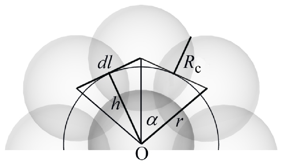
Let us look at Figure 11. Assume the distance between the spheres, i.e. the polygon edge length, is . Since the corrugated rope is wound within a groove, its spheres are at a distance from the center of the axis of the corrugated cylinder. We get
The distance is different when the corrugated rope is wound not within the groove, but on the hill of the corrugated cylinder. Here . In real situations, such as this presented in Figure 9, the corrugated rope runs both in the grooves and on the hills. It is thus reasonable to assume an average . It would be an error to calculate the average as an arithmetic average, since the shape of the hills is not saw-tooth. The hills have the form of circular arcs.

The position of the bead can be parametrized by the angle , whose maximum value is given by
See Figure 12. The average value of is found by integration:
Let us return now to Figure 11. The angle at which the edge is seen from the center is given by
The middle point of the edge is found at the distance from , where
The length of the inscribed arc joining the middle points of two consecutive edges is
Since the arc makes the axis of the smooth rope of radius
the normalized length of the rope segment is
The raw polygonal length of the segment is simply
Now, let us ask the basic question: what is the true ropelength of the segment? It is the length of a piece of a smooth torus (wound tightly on the cylinder of unit radius) seen at angle from the center :
The relationship between the true length , its raw polygonal length , and its inscribed length estimations should be similar to those observed for the true , raw polygonal , and inscribed ropelengths found for knots tightened by SONO. Thus, let us see how the raw polygonal and inscribed rope approximations differ from the true value . To get a clear quantitative estimation of errors that we make using and , we plot the relative deviations and of the raw polygonal and inscribed segment length from its true value. See Figure 13.

By looking at the picture, one can clearly see that underestimates while overestimates the length of the segment. Perhaps an appropriately weighted average of the values could provide a better estimation of the true length. To check this, we solve the equation
Its solution is
The functional dependence of the weight on the edge length looks rather complex, but its plot versus reveals that the dependence is very weak – at , its value is close to 5, but as diminishes, it converges quickly to 4. See Figure 14.

By looking at the plot, one may suspect that the expansion of should have zero order term equal to 4 and much smaller higher order terms. We carried out the expansion to get:
Since the relations between , and in tight knots should be similar to the relations between , and , we arrive to the conclusion that the weighted average
should be almost independent of the edge length and, thus, it should provide a good estimate of the value. To check the hypothesis, we perform a series of tests. First of all, we calculate the weighted average for the trefoil knot, whose and are plotted in Figure 15. Looking at the plot of , one clearly sees that, as expected, it is almost independent of .
| 120 | 0.27243068 | 32.69168 | 32.94095 | 32.7415 |
|---|---|---|---|---|
| 240 | 0.13637831 | 32.73079 | 32.79243 | 32.7431 |
| 480 | 0.06820844 | 32.74005 | 32.75542 | 32.7431 |
| 960 | 0.03410665 | 32.74238 | 32.74622 | 32.7431 |
| 1920 | 0.01705362 | 32.74295 | 32.74391 | 32.7431 |

Similar tests have been performed for the next torus knots: , and .
| 180 | 0.26182883 | 47.12919 | 47.45869 | 47.20 |
|---|---|---|---|---|
| 360 | 0.13105733 | 47.18064 | 47.26225 | 47.20 |
| 720 | 0.06554618 | 47.19325 | 47.21360 | 47.20 |
| 1440 | 0.03277605 | 47.19751 | 47.20261 | 47.20 |
The applicability of the weighted average ropelength to other knots requires further analysis.
| 154 | 0.39748 | 61.21150 | 62.21861 | 61.41 |
|---|---|---|---|---|
| 308 | 0.19921 | 61.35573 | 61.60250 | 61.40 |
| 616 | 0.09966 | 61.39211 | 61.45352 | 61.40 |
| 1232 | 0.04984 | 61.40131 | 61.41663 | 61.40 |
| 188 | 0.40140 | 75.46436 | 76.72711 | 75.72 |
|---|---|---|---|---|
| 376 | 0.20118 | 75.64443 | 75.95430 | 75.71 |
| 752 | 0.10066 | 75.69522 | 75.77243 | 75.71 |
| 1504 | 0.05034 | 75.70902 | 75.72832 | 75.71 |
5. Discussion
Numerical experiments carried out by the SONO algorithm provide us with polygonal knots which can be seen as skeletons of tight knots tied on a corrugated rope. The vertices of the polygonal knots are the centers of the spherical segments of the corrugated tube. As we demonstrated, one can place a smooth tube of a smaller radius inside the corrugated tube to obtain a smooth knot tied within a smooth tube. We know that , the bound on its ropelength, is larger than the ropelength of the ideal knot. In observing the ropelength of the inscribed knots, we see that it converges with the increasing number of vertices to a value , which can be seen as an upper bound for the ropelength of an ideal knot. Determining the value of is a subtle problem and shall not be discussed here; however, by combining the results we obtained for finite with the inscribing algorithm, we are able to find an upper bound for the ropelength of a few ideal knots. For the trefoil knot, the bound equals 32.744, for the knot it equals 47.203, for the knot it equals 61.417 and for the knot it is 75.728. These are the most precise estimations of the upper bounds obtained so far.
As said above, the values we find analyzing the polygonal knots delivered by SONO can be seen as upper bounds for the ropelength of their ideal smooth conformations. But what about the weighted average values ? To see their utility we must adopt the less rigorous point of view of an experimental physicist. The coordinates of the polygonal knots delivered by SONO can be seen as results of measurements carried out on knots tied on the corrugated rope. Analyzing the experimental data, one finds that the knot length calculated according to the raw polygonal length formula systematically increases with while the length calculated according to the inscribed arcs formula systematically decreases with . Plotting the values together, one notices that they converge to a common value: from below, from above. One also finds that, located between the two plots, the plot of their weighted average is almost flat and horizontal. By looking at the values presented in the tables, one can clearly see that provides a good estimate of the ropelength, even at a small number of vertices.
6. Acknowledgments
We thank Maciej Oszwaldowski for indicating the possibility of an analytical analysis of the weighted average algorithm. Pieranski and Baranska were supported under project PB 62 204/04 BW. Rawdon was supported by NSF Grant No. 0296098.
References
- [1] Gregory Buck and Jeremey Orloff. A simple energy function for knots. Topology Appl., 61(3):205–214, 1995.
- [2] J. A. Calvo, K. C. Millett, and E. J. Rawdon, editors. Physical Knots: Knotting, Linking, and Folding Geometric Objects in , volume 304 of Contemporary Mathematics, Providence, RI, 2002. Amer. Math. Soc., Amer. Math. Soc. Physical Knotting and Linking (Las Vegas, NV, 2001).
- [3] Jason Cantarella, Robert B. Kusner, and John M. Sullivan. On the minimum ropelength of knots and links. Invent. Math., 150(2):257–286, 2002.
- [4] M. Carlen, B. Laurie, J. H. Maddocks, and J. Smutny. Biarcs, global radius of curvature, and the computation of ideal knot shapes. In this volume, 2004.
- [5] Y. Diao, C. Ernst, and E. J. Janse van Rensburg. Thicknesses of knots. Math. Proc. Cambridge Philos. Soc., 126(2):293–310, 1999.
- [6] O. Durumeric, R. A. Litherland, E. Rawdon, and J. Simon. Thickness of knots 2. preprint.
- [7] O. Gonzalez and R. de la Llave. Existence of ideal knots. J. Knot Theory Ramifications, 12(1):123–133, 2003.
- [8] Oscar Gonzalez and John H. Maddocks. Global curvature, thickness, and the ideal shapes of knots. Proc. Natl. Acad. Sci. USA, 96(9):4769–4773 (electronic), 1999.
- [9] Vsevolod Katritch, Jan Bednar, Didier Michoud, Robert G. Scharein, Jacques Dubochet, and Andrzej Stasiak. Geometry and physics of knots. Nature, 384(6605):142–145, 1996.
- [10] Robert B. Kusner and John M. Sullivan. On distortion and thickness of knots. In Topology and geometry in polymer science (Minneapolis, MN, 1996), pages 67–78. Springer, New York, 1998.
- [11] R. A. Litherland, J. Simon, O. Durumeric, and E. Rawdon. Thickness of knots. Topology Appl., 91(3):233–244, 1999.
- [12] K. C. Millett and Eric J. Rawdon. Energy, ropelength, and other physical aspects of equilateral knots. J. Comput. Phys., 186(2):426–456, 2003.
- [13] Piotr Pierański. In search of ideal knots. In Ideal knots, pages 20–41. World Sci. Publishing, River Edge, NJ, 1998.
- [14] E. Rawdon. The Thickness of Polygonal Knots. PhD thesis, University of Iowa, 1997.
- [15] Eric J. Rawdon. Approximating the thickness of a knot. In Ideal knots, pages 143–150. World Sci. Publishing, River Edge, NJ, 1998.
- [16] Eric J. Rawdon. Approximating smooth thickness. J. Knot Theory Ramifications, 9(1):113–145, 2000.
- [17] Eric J. Rawdon. Can computers discover ideal knots? Experiment. Math., 12(3):287–302, 2003.
- [18] Jonathan Simon. Physical knots. In Physical knots: knotting, linking, and folding geometric objects in (Las Vegas, NV, 2001), volume 304 of Contemp. Math., pages 1–30. Amer. Math. Soc., Providence, RI, 2002.
- [19] Jana Smutny. Global Radii of Curvature, and the Biarc Approximation of Space Curves: In Pursuit of Ideal Knot Shapes. PhD thesis, EPFL, 2004.
- [20] A. Stasiak, V. Katritch, and L. H. Kauffman, editors. Ideal knots. World Scientific Publishing Co. Inc., River Edge, NJ, 1998.
- [21] Andrzej Stasiak, Jacques Dubochet, Vsevolod Katritch, and Piotr Pieranski. Ideal knots and their relation to the physics of real knots. In Ideal knots, pages 1–19. World Sci. Publishing, River Edge, NJ, 1998.