Constrained Molecular Dynamics Simulations of Atomic Ground-States
Abstract
Constrained molecular dynamics(CoMD) model, previously introduced for nuclear dynamics, has been extended to the atomic structure and collision calculations. Quantum effects corresponding to the Pauli and Heisenberg principle are enforced by constraints, following the idea of the Lagrange multiplier method. Our calculations for small atomic system, H, He, Li, Be, F reproduce the ground-state binding energies reasonably, compared with the experimental data. We discuss also the shell splitting which is expected as a consequence of the e-e correlation.
pacs
34.10.+x; 31.15.QgMolecular dynamics approach is a powerful tool to simulate nuclear heavy ion collisions and atomic collisions, due to its simplicity and ability to take into account the influence of correlations and fluctuations. However, as it is seen in the case of classical trajectory Monte Carlo method ap, truly classical atoms, without constraints due to the Heisenberg and Pauli principle, are unstable. To describe the ground-state properties of the systems with molecular dynamics approach, the pseudo potential is often introduced to simulate the effects of the Heisenberg uncertainty principle and the Pauli exclusion principle kw; cohen0. The method with pseudo potential is known as Fermionic molecular dynamics(FMD) and it is applied to the studies of various atomic processes, in which a fully quantum mechanical dynamical simulation encounters numerical problems difficult to overcome. To give some actual examples, the atom-ion collisions bw, the atomic ionization by laser fields wk, the capture of muons by hydrogen atoms cohen, the formation of antiprotonic atom cohen2 and the ionization cross section calculations gr, all these processes have been investigated using molecular dynamics approach. In particular, Geyer and Rost gr proposed the quasi-classical calculation of the ionization cross section using classical propagation scheme. As the initial state of the target, they use the phase space distributions of the bound electrons which are directly obtained from quantum mechanical wave functions through the Wigner transformation. There they mention the importance of the energy spread of the phase space distributions.
Meanwhile, a constrained molecular dynamics (CoMD) approach has been proposed to treat fermionic properties of the nucleons in nuclei pmb. The approach has been successfully applied to study the Equation of State of the quark system as well tb. In this approach, the Pauli exclusion principle is accomplished by restricting the phase space occupancy to values less or equal to 1 bgm. The equation of motion with the constraints for each electron is derived on the basis of Lagrange multiplier method for constraints. The constraint of CoMD approach is thought as an alternative to the pseudo potential and can be easily extended to the case of the Heisenberg uncertainty principle as well. The constraints play the role of a “dissipative term” in the classical equation of motion and lead the system to its ground-state. But in CoMD, at variance with FMD approaches, the “dissipative term” can increase or decrease the energy of the system depending on the phase space occupation.
In this brief report, we apply CoMD to atomic systems for the purpose of determining their ground-states configurations. Particularly, we discuss some properties of ground-states atoms, i.e., binding energies (the total electronic energies) and radial positions of the bound electrons. We discuss also the energy spread (variance of the binding energy) and radial variance of each bound electron as well. In our approach, we prepare the ensemble of initial configurations. The binding energies and radial positions of the electrons in the systems are calculated as averaged values over the ensembles. Our approach is sufficient to obtain stable atomic ground-states providing their atomic energies fairly accurately. Using the obtained ensembles of initial states which occupy different points in the phase space, molecular dynamics simulation with constraints for the atomic collision has been performed and applied to nuclear fusion enhancement factor calculations of D+ reaction for astrophysical interests kb.
We describe the essence of CoMD briefly. In classical molecular dynamics(CMD) one solves the Hamilton equations, i.e.,:
| (1) |
where we use relativistic kinematics: , and
| (2) |
are the energy, the mass and the potential of the -th electron, respectively. Here, is the charge of the electron and is the charge of electron(for ) or nucleus(for ). The total Hamiltonian is written down as .
The shortcoming of the approach is the lack of the Pauli exclusion principle. CoMD gives a possibility to overcome the shortcoming. To take the feature of the Pauli blocking into account, we use the Lagrange multiplier method for constraints. Our constraints which correspond to the Pauli blocking is in terms of the occupation probability and can be directly related to the distance of two particles, i.e., , in the phase space. Here and . The relation is fulfilled, if , where , refer only to electrons and are their spin projection. We can easily extend the approach to the Heisenberg principle where the constraint is expressed as , where , and refer to the electrons and the nucleus. Using these constraints, the Lagrangian of the system can be written as
| (3) |
where and are Lagrange multipliers for Pauli and Heisenberg principle respectively. The variational calculus leads to:
| (4) | ||||
| (5) |
From physical considerations we expect that the Pauli principle is stronger than the Heisenberg principle for the two closest identical electrons in the phase space, i.e., the particles and for which is smallest. While the Heisenberg principle must be enforced especially among the electrons and the nucleus. Thus we restrict the summations in eqs. (3)-(5) to those particles only.
In order to obtain the atomic ground-state configuration, we perform the time integration of the eqs. (4) and (5). The values of and are determined depending on the magnitude of . If is (smaller)larger than , has positive(negative) sign, changing the phase space occupancy of the system. The constraints work as the “dissipative term” in the case of the pseudo potential approach and lead automatically to the minimum energy, i.e., the ground-state of the system. The difference being that in the case of the model with the pseudo potential, a dissipative term decreases the total energy. In our case the total energy decreases or increases depending on the phase space occupancy.
The electron configurations at the beginning of the time integration are prepared in the following way. In the case of even number of bound electrons, we locate a pair of them at the opposite points respect to the nucleus in the phase space. In this way, the center of mass of the electrons coincides with the position of the nucleus, i.e., total momentum of the electrons is zero. We do the same procedure for the odd-number electrons atom, excluding an electron which is the outermost. Thus, at the beginning of the time integration we have an ensemble of electron configurations which occupy different points in the phase space microscopically. The integration of the eqs. (4) and (5) is performed using Hermite integration scheme which is efficient and enables integration with high precision. The scheme adopts variable and individual time-steps for each electron ma. Considering the nucleus rest frame, The binding energy of the atom is determined by
| (6) |
where is the number of the events in the ensemble. The radial coordinates of the electron () is given by
| (7) |
The binding energies and the radial coordinates of the electron of the atoms are calculated as an averaged value over the ensemble of events.
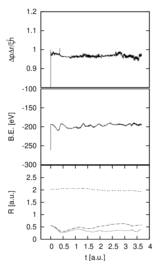
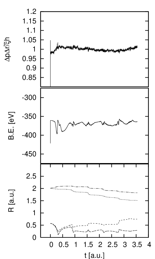
We have applied the model to hydrogen, helium, lithium, beryllium, fluorine atoms. Fig. 1 and Fig. 2 show that the systems converge to their ground-state in the illustrative cases of lithium and beryllium atoms, respectively. The top panels show the time development of the average of over all pair of particles and over events in the ensemble, we write it as . The middle panels and the bottom ones show the average of binding energy and the radial coordinates of the electrons, respectively, over events. In the bottom panels each line corresponds to the radius of each bound electron. Due to the constraints these values oscillate as a function of time and converge after some time. We determine the binding energy and the radius by taking the average over not only events but also over time.
We summarize our results of the ground-state energies and the radial coordinates of the bound electrons for small atomic systems in Table 2 and 2, respectively. For the purpose of utilizing the atomic configuration to collision calculations, the comparison between our results and the ones from quantum mechanical Hartree-Fock(HF) is suggestive. In Table 2 together with the ground-state energies from our method, results from the FMD cohen1, HF fischer methods and experimental values ben are shown. Since we determine the binding energies as an average of many events, our results have a variance , also included in the tables. We obtain ground-state binding energies in good agreement with experimental data within variances. In Table 2 we compare our results of the radial coordinates of the electrons() for each atoms with FMD and HF methods. The results from FMD which are obtained using different parameter sets are shown in two columns(FMD 0 cohen0 and FMD 1 cohen1). The column FMD 1 is with the optimized parameter sets. Note that our method gives smaller values as than those from HF method. However one should notice that while comparison of our approach to FMD is direct since they are all semi-classical molecular dynamics, thus the definition given in eqs. (6), (7) are exactly the same. On the other hand in the HF approach there are no “events”, the calculated values of HF are obtained through a smooth probability distribution, which is not the case for our model where we have -functions. Furthermore symmetries imposed to the system will be preserved in HF, indeed they might be destroyed in CoMD because of correlations. We give an example of the Be case; initially we distributed the electrons pairwise, one opposite to the other respect to the nucleus both in the coordinate and momentum space, as stated above. This initial symmetry is broken in the simulation because of e-e correlation, nevertheless one can recognize two major shells within the variance in the results. Certainly even in our calculations we can impose such a symmetry. In Tables 2 and 2 the numbers in parenthesis show in the case where we impose that electrons move pairwise opposite locations in the phase space, i.e., they are forced to keep the initial symmetries. Such a calculation gives a very similar as in the absence of forced symmetry, but now two major shells are clearly identified. From the comparison of these two cases it is obvious the splitting of the shells when relaxing the initial symmetry.
| CoMD | FMD 1 | HF | experimental | |
|---|---|---|---|---|
| H | 13.3 1.8 | 13.61 | 13.61 | 13.6 |
| He | 79.1 6.9 | 77.57 | 77.87 | 79.1 |
| Li | 196.8 15. | 197.61 | 202.26 | 203.6 |
| Be | 371.2 27. (385.3 29.)11 1 with forced symmetry | 395.63 | 396.56 | 399.4 |
| F | 2560.3 192. | 2408.3 | 2705.1 | 2717.4 |
| CoMD | FMD 0 FMD 1 | HF | ||
|---|---|---|---|---|
| H | 1.0 0.2 | 1.0 1.0 | 1.0(1s) | |
| He | 0.55 0.09 | 0.5714 0.6139 | 0.9273(1s) | |
| 0.60 0.1 | 0.5714 0.6139 | |||
| Li | 0.34 0.1 | 0.3506 0.3818 | 0.5731(1s) | |
| 0.5 0.2 | 0.3673 0.3885 | 3.8737(2s) | ||
| 2.0 0.6 | 1.4419 4.0604 | |||
| Be | 0.27 0.13 (0.36 0.17)22 2 same as in Table 2,with forced symmetry | 0.2565 0.2687 | 0.4150(1s) | |
| 0.47 0.20 (0.36 0.17) | 0.2565 0.2687 | 2.6494(2s) | ||
| 1.63 0.45 (1.60 0.34) | 0.9458 2.9738 | |||
| 1.83 0.47 (1.60 0.34) | 0.9458 2.9738 | |||
| F | 0.15 0.09 | 0.2625 | 0.1757(1s) | |
| 0.30 0.09 | 0.2624 | 1.0011(2s) | ||
| 0.41 0.05 | 0.2622 | 1.0848(2p) | ||
| 0.48 0.05 | 0.2622 | |||
| 0.55 0.07 | 0.2668 | |||
| 0.61 0.07 | 0.2671 | |||
| 0.69 0.07 | 0.6931 | |||
| 0.75 0.07 | 0.6952 | |||
| 0.87 0.1 | 0.7818 |
We have presented results of Constrained molecular dynamics approach to describe the atomic ground-states configurations. We calculated the binding energies and the radial coordinates of the electrons in atoms. The total electronic energies for the ground-state atoms are given rather accurately, At last we stress that the intent of the CoMD simulation of the atomic systems is to applying it to the collision calculations and determining the Equation of State of matter at very low temperatures where quantum effects play a decisive role.
We thank Prof. J.S. Cohen for providing us his data.
References
- (1) R. Abrines and I.C. Percival, Proc. Phys. Soc. 88, 861(1966); S. Keiler, H. Ast, and R.M.Dreizler J. Phys. B 26, L737(1993).
- (2) C.L. Kirschbaum, and L. Wilets, Phys. Rev. A 21, 834(1980).
- (3) J.S. Cohen, Phys. Rev. A 51, 266(1994); J.S. Cohen, Phys. Rev. A 57, 4964(1997).
- (4) W.A. Beck, and L. Wilets, Phys. Rev. A 55, 2821(1997).
- (5) D.A. Wasson, and S.E. Koonin, Phys. Rev. A 39, 5676(1988).
- (6) J.S. Cohen, J. Phys. B 31, 833(1998).
- (7) J.S. Cohen, Phys. Rev. A 56, 3583(1997).
- (8) T. Geyer and JM. Rost J. Phys. B 35, (6): 1479(2002).
- (9) M. Papa, T. Maruyama, and A. Bonasera, Phys. Rev. C 64, 024612(2001).
- (10) S. Terranova, and A. Bonasera, Phys. Rev. C 70, 024906 (2004).
- (11) A. Bonasera, F. Gulminelli, and J. Molitoris, Phys. Rep. 243, 1 (1994).
- (12) S. Kimura, and A. Bonasera, Phys. Rev. Lett. 93, 262502 (2004).
- (13) J. Makino, and S. J. Aarseth, PASJ 44, 141(1992).
- (14) J.S. Cohen, (private communication), J.S. Cohen, Phys. Rev. A 69, 022501(2004).
- (15) C. F. Fischer, At. Data Nucl. Data Tables 12, 87 (1973).
- (16)
These binding energies are obtained from the measured ionization energies of atoms given in
the web site:
http://www.webelements.com/