Destabilization of the thermohaline circulation by transient perturbations to the hydrological cycle
Abstract
We reconsider the problem of the stability of the thermohaline circulation as described by a two-dimensional Boussinesq model with mixed boundary conditions. We determine how the stability properties of the system depend on the intensity of the hydrological cycle. We define a two-dimensional parameters’ space descriptive of the hydrology of the system and determine, by considering suitable quasi-static perturbations, a bounded region where multiple equilibria of the system are realized. We then focus on how the response of the system to finite-amplitude surface freshwater forcings depends on their rate of increase. We show that it is possible to define a robust separation between slow and fast regimes of forcing. Such separation is obtained by singling out an estimate of the critical growth rate for the anomalous forcing, which can be related to the characteristic advective time scale of the system.
1 Introduction
The thermohaline circulation (THC) plays a major role in the global circulation of the oceans as pictured by the conveyor belt scheme (Weaver and Hughes 1992; Stocker 2001). The currently accepted picture is that the meridional overturning and the associated heat and freshwater transports are energetically sustained by the action of winds and tides, controlling turbulent mixing in the interior of the ocean (Munk and Wunsch 1998; Rahmstorf 2003; Wunsch and Ferrari 2004). However, for climatic pourposes, many authors have succesfully assumed a dependence of the strength of the THC from the meridional gradients in the buoyancy of the water masses (Stommel 1961; Weaver and Hughes 1992; Tziperman et al. 1994; Marotzke 1996; Rahmstorf 1996; Gnanadesikan 1999; Stocker et al. 2001).
The present day THC of the Atlantic Ocean is characterized by a strongly asymmetric structure. Deep convection is observed at high latitudes in the northern hemisphere. The water masses formed in the northern regions can be followed as they cross the equator and observed as they connect with the other major basins of the world ocean (Weaver and Hughes 1992; Rahmstorf 2000; Rahmstorf 2002; Stocker et al. 2001). Idealized and realistic coupled GCM experiments have shown that such equatorial asymmetry may be a consequence of the large scale oceanic feedbacks leading to the existence of multiple equilibria (Bryan 1986; Manabe and Stouffer 1988; Stocker and Wright 1991; Manabe and Stouffer 1999a; Marotzke and Willebrand 1991; Hughes and Weaver 1994). The equatorial asymmetry is also responsible for a large portion of the the global poleward heat transport (Broecker 1994; Rahmstorf and Ganopolski 1999; Stocker 2000; Stocker et al. 2001). Consequently, large climatic shifts are often associated with important changes in the large scale oceanic circulation. On a paleoclimatic perspective, major climatic shifts may be associated with the complete shutdown of the THC (Broecker et al. 1985; Boyle and Keigwin 1987; Keigwin et al. 19994; Rahmstorf 1995; Rahmstorf 2002).
In fact, the THC is sensitive to changes in the climate since the North Atlantic Deep Water (NADW) formation is affected by variations in air temperature and in precipitation in the Atlantic basin (Rahmstorf and Willebrand 1995; Rahmstorf 1996). With respect to the present climate change, most GCMs have shown that the changes in radiative forcing caused by the on-going modification of the greenhouse gases in the atmosphere could imply a weakening of the THC. Large increases of the moisture flux and/or of the surface air temperature in the deep-water formation regions could inhibit the sinking of the water in the northern Atlantic (Weaver and Hughes 1992; Manabe and Stouffer 1993; Rahmstorf 1997; Rahmstorf 1999b; Rahmstorf 1999a; Rahmstorf 2000; Wang et al. 1999a; Wang et al. 1999b). Moreover, models of different level of complexity, from box models (Tziperman and Gildor 2002; Lucarini and Stone 2003a; Lucarini and Stone 2003b), to EMICs (Stocker and Schmittner 1997; Schmittner and Stocker 1999) to GCMs (Stouffer and Manabe 1999; Manabe and Stouffer 1999a; Manabe and Stouffer 1999b; Manabe and Stouffer 2000) have shown how the rate of increase of forcing may be relevant for determining the response of the system. In particular Stocker and Schmittner 1997 have performed a systematic analysis of the stability of the meridional overturning circulation as a function of the climate sensitivity and of the rate of CO2 increase. However they made no explicit reference as to the mechanism driving the response of their coupled model.
In this work we study the THC stability using a simplified 2D Boussinesq ocean model, which has been presented in Artale et al. 2002. Two-dimensional models have been widely adopted (Cessi and Young 1992; Vellinga 1996) and have proved their ability in describing the most relevant feedbacks of the system (Dijkstra and Neelin 1999). Moreover, the low computational cost of such models permits extensive parametric studies. Our work wishes to bridge both in terms of methodology and results the studies performed with simplified models with the more physically sensible analyses performed with EMICs and GCMs. We explicitly analyze what is the role of the rates of changes of the hydrological forcing in determining the response of the system. In particular we determine, for a given initial state and a given rate of increase of the forcing, which are the thresholds in total change of the forcing beyond which destabilization of the THC occurs. The treatment of a wide range of temporal scales for the increase of the forcing allows us to join on naturally and continuously (Lucarini and Stone 2003a; Lucarini and Stone 2003b) the analysis of quasi-static perturbations, which have been usually addressed with the study of the bifurcations of the system (Rahmstorf 1995; Rahmstorf 1996; Stone and Krasovskiy 1999; Scott et al. 1999; Wang et al. 1999a; Titz et al. 2002b; Titz et al. 2002a), with the study of the effects of very rapid perturbations (Rahmstorf 1996; Scott et al. 1999; Wiebe and Weaver 1999), which are usually differently framed.
Our paper is organized as follows. In section 2 we provide a description of the model we adopt in this study. In section 3 we explore the parameters space descriptive of the hydrology of the system by considering quasi-static perturbations. We determine which hydrological patterns are compatible with multiple equilibria and which hydrological patterns define a unique stationary state. In section 4 we extend the analysis to time-dependent perturbations. We analyze the temporal evolution of finite amplitude modifications of the hydrological cycle that are able to destabilize the equilibria of this advective system. We propose a simple relation between an estimate of the critical rate of increase of forcing, which divides robustly slow from fast regimes, with an estimate of the characteristic advective time scale of the system. In section 5 we present our conclusions. In appendix A we present the dependence of the THC strength on the value of the vertical mixing coefficient.
2 The model
We consider the two-dimensional convection equations in the Boussinesq approximation. The motion is forced by buoyancy gradients only: gravity is the only external force, while Earth rotation is not explicitly considered. Buoyancy gradients are generated in the model by imposing heat and freshwater fluxes at the top boundary. Such fluxes are assumed to be representative of the interactions with the overlying atmosphere.
We adopt a linearized equation of state for the sea water:
| (1) |
where the values of the coefficients of thermal expansion and haline contraction have been chosen in order to provide a good approximation over a quite large range of salinity and temperature. The linear approximation is commonly adopted in conceptual models. However, we note that analyses performed on simple models show that small nonlinearities may induce self-sustained oscillations for the THC (Rivin and Tziperman 1997). Such nonlinearities in the equation of state might be especially relevant for the high latitude areas, since the well-known cabbeling effect occurs at low temperatures.
The geometry of the model is descriptive of the Atlantic ocean, where we assume a depth of , an effective east-west extension of , and a north-south extension of () and a total volume . The only active boundary of the model is the air-sea interface.
We select a relatively coarse uniform resolution with grid points, where and refer to the number of the horizontal and vertical grid points, respectively, in order to meet the computational requirements needed for performing a parametric study.
A well known property of the THC system is the existence of regimes of multiple equilibria. When equatorially symmetric surface forcing is applied at the surface, the equilibria of the system fall into three well-distinct classes. One class is characterized by the presence of two equatorially symmetric thermally direct cells, where the deep water is formed at high latitudes. Another class is characterized by equatorially symmetric salinity driven cells, where deep water is formed in the equatorial region. Equilibria belonging to these two classes are observed when either surface thermal or haline buoyancy forcings are largely dominant, respectively. When the two forcings have comparable intensity, multiple equilibria regimes - which constitute a third class - appear. In this case, the equilibria are characterized by the dominance of one overturning cell. If also geometry is symmetric with respect to the equator, the two equilibria have odd parity and map into each other by exchanging the sign of the latitude.
a Boundary conditions
The boundary condition for the sea surface salinity is defined in terms of the imposed atmospheric freshwater flux affecting the surface grid box of volume :
| (2) |
where we indicate the value of the bulk variable at the grid point with and the value of the interface variable at the grid point with . We underline that, in order to simplify the expressions, in equation (2) (and in the following ones) we have not explicitly adopted a discrete notation for the time variable.
We emphasize that in expression (2) we have neglected the contribution in terms of mass of the freshwater flux to the ocean (Marotzke 1996).
We divide the water basin into three distinct regions by using a suitable analytical expression of the freshwater flux. The equatorial region (region E) is characterized by a net atmospheric export of freshwater, while the northern and southern high latitude regions (regions and , respectively) are characterized by a positive atmospheric freshwater budget. We then consider the following functional form for the surface freshwater flux:
| (3) |
where:
| (4) |
The definition of is such that and are respectively the value of the total net atmospheric freshwater fluxes into regions and , while is constrained in order to have conservation of the salinity of the ocean. This latter condition is needed to allow the system to reach equilibrium states. Therefore, the ocean conserves its average salinity . Since the atmospheric freshwater budgets for the Atlantic ocean are thought to be positive for the regions and (Baumgartner and Reichel 1975), we consider the case . Three relevant examples of surface freshwater flux are depicted in figure 1.
The sea surface temperature is restored to a time-independent climatological temperature field with a newtonian relaxation law:
| (5) |
where the constant describes the efficiency of the process. Such very simplified ocean-atmosphere coupling (Marotzke and Stone 1995; Marotzke 1996) synthetically describes the combined effects of radiative heating-cooling and of the atmospheric latent and sensible heat meridional transport. The climatological temperature profile profile is set with the following equatorially symmetric analytical form:
| (6) |
where is the imposed equator-to-pole temperature gradient and is the average value of . In accordance to definition of the , , and regions with respect to their atmospheric freshwater budget, we observe that regions and are cold at surface, i.e. is lower than , while the region is warm at surface, i.e. is larger than .
Since in our work we explore the stability of the THC with respect to the hydrology of the system, we keep fixed the parameters determining the restoring temperature profile . We set , since it represents a reasonable average surface climatological temperature, and we choose , which corresponds to forcing the surface equator-to-pole temperature gradient to be . Such a choice also implies that the average is in the two high latitude regions and and is in the equatorial region . Furthermore, following the parameterization proposed by Marotzke 1996, we choose the restoring constant , which is reasonable for the description of the temperature relaxation of the uppermost of the ocean.
3 Quasi-static hysteresis and multiple equilibria
a Symmetric case:
We start by considering the existence of a region of multiple equilibria in the space of parameters that defines the hydrology of the system, i.e. the plane. The surface thermal forcing is kept fixed. In the space of parameters that we are considering, symmetric forcings constitute the bisectrix of the plane. The allowed circulation patterns change when adjusting the parameters along the bisectrix, as discussed in section 2. For a weak hydrological cycle (), we observe a stable symmetric circulation with downwelling at high latitudes. If the hydrological cycle is very strong (), we obtain a stable symmetric circulation with downwelling of warm, saline water at the equator. In the intermediate regimes (), the system has multiple equilibria. For later convenience, we define , which corresponds to an average hydrological cycle. The described equilibria are depicted in figures 2a), 2b), 3a), and 3b) respectively. The two points and are bifurcation points in the one-dimensional subspace (Dijkstra and Neelin 1999). We consider the northern sinking equilibrium state (note that northern and southern sinking patterns are equivalent in these terms) realized for as the reference state of the system.
b General case:
The study of the multiple equilibria states can be extended to the case of non-symmetric forcings, i.e. . We wish to obtain an estimate of the shape of the domain in the plane where the system has multiple equilibria.
Since, apart from the freshwater flux boundary conditions, the model is wholly symmetric with respect to the equator, we expect that any property of the system is invariant for exchange of and , so that we have that is a priori symmetric with respect to the bisectrix.
A fundamental property of the region is that, if we start from a point belonging to and change quasi-statically and along a closed path so that the point remains inside , we get back to the initial equilibrium state. Instead, if the closed path crosses the boundary of , the initial equilibrium state may not be recovered at the end of the loop, since the final state depends on the path.
As a starting position of the loop, we consider a northern sinking equilibrium corresponding to one of the stable states of the point on the bisectrix. By definition, such point belongs to . However, the initial position of the loop - if belonging to - is not relevant in determining the shape of the region of multiple equilibria.
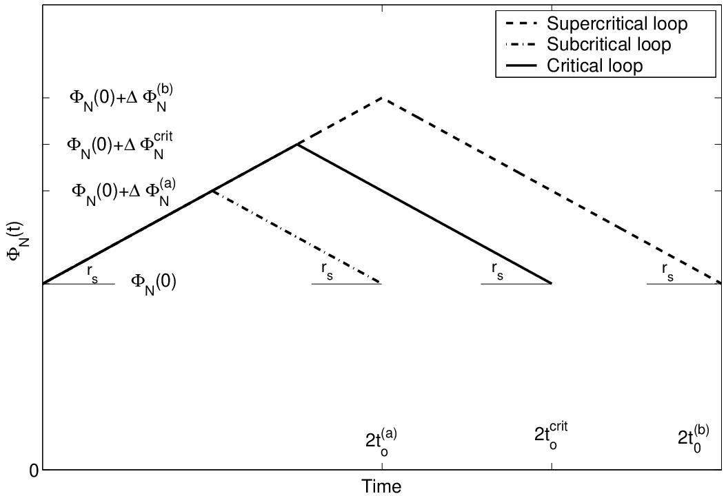
We increase the value of at a given slow constant rate over a time and then decrease it back to the initial value at the rate . By slow rate we mean that ; we select . If the initial state is not recovered at the end of the integration, we deduce that the path has crossed the boundary of . By bisection, we can determine the critical value , which determines as belonging to the boundary of . A schematization of this procedure is depicted in figure 4a). By changing the initial point along the considered segment of the bisectrix, we are able to define the whole boundary of above the bisectrix with a good degree of precision. Then, the symmetry properties of allow us to easily deduce the portion of its boundary lying below the bisectrix. In figure 5 we present the estimate for the the boundary of the bistable region obtained following this strategy.
We conclude that the boundary of is constituted by the bifurcation points of the system. We note that in the more general case of the 2D plane, and result to be cusp points (Dijkstra 2001).
4 Effects of transient perturbations
The analysis we have performed captures the equilibrium properties of the system, but is not sufficient to gain insight on the response of the system to transient changes in the forcings, which in general can range from instantaneous to quasi-static perturbations. Such sort of problems has been first investigated in the seminal paper by Stocker and Schmittner 1997 with the purpose of determining how efficiently the negative feedbacks of the system can counteract external perturbations, depending on the temporal patters of the destabilizing forcings.
In our case, it is reasonable to expect that, if we change at a finite rate, the system can destabilize before reaching the boundary of . In fact, a fast perturbation can overcome the ability of the advective feedback to stabilize the system. We also expect that the faster the perturbation, the stronger such effect, i.e. the smaller the total perturbation required to obtain destabilization.
As in the previous case, the analysis starts by considering as initial equilibria the northern sinking states under symmetric forcing. In this case, we increase the value of at a constant rate over a time , we let the system adjust for a time , so that transients can die out, and then decrease back to the initial value at the slow rate , corresponding to a quasi-static change. We schematically depict such strategy for three different values of in figure 4b). If at the end of the process the initial state is not recovered and southern sinking state is instead realized, the system has made a transition to the other branch of the multiple equilibria. Depending on the choice of , we obtain different values for the critical perturbation causing such transition. Along the lines of the quasi-static analysis, varying the initial point, we can obtain for each value of a curve which describes the critical perturbations.
In figure 6 we report the curves obtained by selecting, from fast to slow, , , , , and .
If we select , we obtain by definition the previously described upper branch of the boundary of depicted in figure 5, since the presence of the relaxing time is not relevant.
On the other extreme, if we apply instantaneous changes of (), we obtain information on the minimum change in that is needed to destabilize the system for any initial state having symmetric surface forcing. In fact, the corresponding curve is the closest to the bisectrix.
Considering intermediate values of , we obtain consistently that the curves of the critical perturbations lye within the two extremes obtained with and . Moreover, we have that the curves are properly ordered with respect to the value of , i.e. the smaller , the closer the corresponding curve to the upper branch of the boundary of .
Previous studies, albeit performed with coupled EMICs, obtain a qualitatively similar dependence of thresholds on the rate of increase of the forcings (Stocker and Schmittner 1997; Schmittner and Stocker 1999), while in other studies (on GCMs) where the full collapse of the THC is not obtained, it is nevertheless observed that the higher the rate of increase of the forcing, the larger the decrease of THC realized (Stouffer and Manabe 1999).
The most important result is that we can identify two separate regimes. If the surface forcing changes with a rate faster than , the response of the system is virtually identical to the case of instantaneous changes. On the other side, if the rate of change is smaller that , the response of the system is very close to the case of quasi-static perturbations. The curve corresponding to is geometrically about midway between these two regimes and is not patched to either. We have that the response of the system to varying external perturbations dramatically changes when the time scale of the variation of the external forcing changes by only one order of magnitude. Therefore, we can interpret as an estimate of the critical rate of change of the hydrology of the system.
It follows that with we identify a relation between the class of changes in the external forcing that distinctively affect the stability of the system and the internal time scale of the system.
The previous results prove to be robust with respect to changes in the freshwater forcing of the initial states. As an example, in figure 7 we show the results of a similar analysis referring to initial states having non-symmetric surface freshwater forcing ().
We explored the behavior of the system in the plane considering only changes in for computational convenience. Nevertheless, coherent results can be obtained by changing both parameters. In this case has to be interpreted as the sum of the absolute values of the rates of change of the two parameters.
Changing the parameter implies a change in the values of and , since the meridional gradient of the total buoyancy forcing is changed. However, the response of the THC to transient perturbations does not change qualitatively. Instead, figures 5-7 must be rescaled linearly with the proper values of and . Such linear relation is a direct consequence of the use of a linearized equation of state for the sea water.
5 Conclusions
This work provides a complete analysis of the stability of the ocean system under examination with respect to perturbation to the hydrological cycle. We have provided a simple description of the profile of the net freshwater flux into the ocean which is fully specified when only two parameters, which are related to the total freshwater budget of the two high-latitudes regions, are specified.
We have first analyzed the bifurcations of the symmetric system, which might be taken as the prototype of a system that has equal probabilities of falling in two different equilibrium configurations. We have found that the system is characterized by two bifurcations, which delimitate a domain of multiple equilibria.
We have then extended the study to the general case where asymmetries in the hydrology are considered. We have produced a two-dimensional stability graph and have pointed out the presence of a region where multiple equilibria are realized. Our results summarize the information that can be obtained with multiple hysteresis studies.
In this study we emphasize that the rate at which a perturbation in the hydrological cycle is applied to a simple model of the THC may dramatically affect its stability. When general time-depends perturbation to the hydrological cycle are considered, we obtain that the shorter the time scale of the forcing, the smaller the total perturbation required to disrupt the initial pattern of the circulation. The observed relevance of the temporal scale of the forcing in determining the response of our system to perturbations affecting the stability of the THC agrees with the findings of Tziperman and Gildor 2002, Lucarini and Stone 2003a; Lucarini and Stone 2003b for box models, of Stocker and Schmittner 1997 and Schmittner and Stocker 1999 in the context of EMICSs, and of (Manabe and Stouffer 1999a), Manabe and Stouffer 1999b, Manabe and Stouffer 2000, and Stouffer and Manabe 1999 in the context of GCMs. Moreover, the saturation and patching effect observed for slowly and rapidly increasing perturbations, which allows the definition of slow and fast regimes, respectively, agrees qualitatively with the findings of Lucarini and Stone 2003a; Lucarini and Stone 2003b for box models, and resembles some of the results - albeit obtained with a coupled model and considering CO2 increases - presented in Stocker and Schmittner 1997 and in Schmittner and Stocker 1999.
The main conceptual improvement we propose in this work is the existence of a relation between the critical rate of change of the forcing and the characteristic advective time scale of the system.
We notice that the advective time scale results to depend on the inverse of the square root of , as discussed in appendix A. Therefore, a very important consequence of this analysis is that the efficiency of the vertical mixing might be also one of the key factors determining the response of the THC system to transient changes in the surface forcings. Future work should specifically address the details of the functional dependence of the critical rate on the the vertical diffusivity.
Other relevant improvements to the present study could be the adoption of a more complex ocean model, descriptive of other ocean basins, as well as the consideration of a simplified coupled atmosphere-ocean model, where the effects of the radiative forcing can be more properly represented.
Acknowledgment
We wish to thank for technical and scientific help Fabio Dalan, Antonello Provenzale, Peter H. Stone, and Antonio Speranza.
Appendix A. Relevance of the vertical diffusivity
The vertical diffusivity , or, equivalently, the diapycnal diffusivity , is the critical parameter controlling the maximum THC strength in ocean models (Bryan 1987; Wright and Stocker 1992). On the other hand, an estimate of its value in the real ocean is a subject of current research (Gregg et al. 2003). Scaling theories proposing a balance between vertical diffusion and advection processes suggest, in the case of three-dimensional hemispheric model of the Atlantic ocean, a power law dependence (Zhang et al. 1999; Dalan et al. 2004). In the case of two-dimensional models, the expected dependence is (Knutti et al. 2000). This relation is verified in our model in the range (figure 8). In this study, the value of has been selected so that the corresponding northern sinking equilibrium state characterized by an hydrological cycle determined by has an overturning circulation . With this choice of we can define a characteristic time scale for the system as . Similarly, if we change over the range shown in figure 8, the advective time-scale would range over the interval . These considerations will be useful in the final discussion of our results. Given the parameters chosen for our simulations, our model integrations estimate and , so that results to be .
References
- Artale et al. (2002) Artale, V., S. Calmanti, and A. Sutera, 2002: Thermohaline circulation sensitivity to intermediate-level anomalies. Tellus A, 54, 159–174.
- Baumgartner and Reichel (1975) Baumgartner, A. and E. Reichel, 1975: The World Water Balance. Elsevier, New York.
- Boyle and Keigwin (1987) Boyle, E. A. and L. Keigwin, 1987: North Atlantic thermohaline circulation during the past 20000 years linked to high-latitude surface temperature. Nature, 335, 335.
- Broecker (1994) Broecker, W. S., 1994: Massive iceberg discharges as triggers for global climate change. Nature, 372, 421.
- Broecker et al. (1985) Broecker, W. S., D. M. Peteet, and D. Rind, 1985: Does the ocean-atmosphere system have more than one stable mode of operation. Nature, 315, 21.
- Bryan (1986) Bryan, F., 1986: High-latitude salinity effects and interhemispheric thermohaline circulations. Nature, 323, 301.
- Bryan (1987) — 1987: Parameter sensitivity of primitive equation ocean general circulation models. J. Phys. Oceanogr., 17, 970–985.
- Cessi and Young (1992) Cessi, P. and W. R. Young, 1992: Multiple equilibria in two-dimensional thermohaline flow. J. Fluid Mech., 241, 291–309.
- Dalan et al. (2004) Dalan, F., P. H. Stone, I. Kamenkovich, and J. R. Scott, 2004: Sensitivity of climate to dyapicnal diffusion in the ocean - Part I: Equilibrium state. J. Climate, submitted.
- Dijkstra (2001) Dijkstra, H. A., 2001: Nonlinear Physical Oceanography. Kluwer, Dordrecht.
- Dijkstra and Neelin (1999) Dijkstra, H. A. and J. D. Neelin, 1999: Imperfections of the thermohaline circulation: Multiple equilibria and flux-correction. J. Climate, 12, 1382–1392.
- Gnanadesikan (1999) Gnanadesikan, A., 1999: A simple predictive model for the structure of the oceanic pycnocline. Science, 263, 2077–2079.
- Gregg et al. (2003) Gregg, M. C., T. B. Sanford, and D. P. Winkel, 2003: Reduced mixing from the breaking of internal waves in equatorial waters. Nature, 422, 513–515.
- Hughes and Weaver (1994) Hughes, T. C. M. and A. J. Weaver, 1994: Multiple equilibrium of an asymmetric two-basin model. J. Phys. Ocean., 24, 619.
- Keigwin et al. (19994) Keigwin, L. D., W. B. Curry, S. J. Lehman, and S. J. S., 19994: The role of the deep ocean in North Atlantic climate change between 70 and 130 ky ago. Nature, 371, 323.
- Knutti et al. (2000) Knutti, R., T. W. Stocker, and D. G. Wright, 2000: The effects of subgrid-scale parameterizations in a zonally averaged ocean model. J. Phys. Ocean., 54, 2738–2752.
- Lucarini and Stone (2003a) Lucarini, V. and P. H. Stone, 2003a: Thermohaline circulation stability: a box model study - Part I: uncoupled model. J. Climate, submitted.
- Lucarini and Stone (2003b) — 2003b: Thermohaline circulation stability: a box model study - Part II: coupled model. J. Climate, submitted.
- Manabe and Stouffer (1988) Manabe, S. and R. J. Stouffer, 1988: Two stable equilibria coupled ocean-atmosphere model. J. Climate, 1, 841.
- Manabe and Stouffer (1993) — 1993: Century-scale effects of increased atmospheric CO2 on the ocean-atmosphere system. Nature, 364, 215.
- Manabe and Stouffer (1999a) — 1999a: Are two modes of thermohalince circulation stable? Tellus, 51A, 400.
- Manabe and Stouffer (1999b) — 1999b: The role of thermohaline circulation in climate. Tellus, 51A-B(1), 91–109.
- Manabe and Stouffer (2000) — 2000: Study of abrupt climate change by a coupled ocean-atmosphere model. Quat. Sci. Rev., 19, 285–299.
- Marotzke (1996) Marotzke, J.: 1996, Analysis of thermohaline feedbacks. Decadal Climate Variability: Dynamics and predicatibility, Springer, Berlin, 333–378.
- Marotzke and Stone (1995) Marotzke, J. and P. H. Stone, 1995: Atmospheric transports, the thermohaline circulation, and flux adjustments in a simple coupled model. J. Phys. Ocean., 25, 1350–1360.
- Marotzke and Willebrand (1991) Marotzke, J. and J. Willebrand, 1991: Multiple equilibria of the global thermohaline circulation. J. Phys. Ocean., 21, 1372.
- Munk and Wunsch (1998) Munk, W. and C. Wunsch, 1998: Abyssal recipes II. Energetics of the tides and wind. Deep-Sea Res., 45, 1976–2009.
- Rahmstorf (1995) Rahmstorf, S., 1995: Bifurcations of the Atlantic thermohaline circulation in response to changes in the hydrological cycle. Climatic Change, 378, 145.
- Rahmstorf (1996) — 1996: On the freshwater forcing and transport of the Atlantic thermohaline circulation. Clim. Dyn., 12, 799.
- Rahmstorf (1997) — 1997: Risk of sea-change in the atlantic. Nature, 388, 528.
- Rahmstorf (1999a) Rahmstorf, S.: 1999a, Rapid oscillation of the thermohaline ocean circulation. Reconstructing ocean history: A window into the future, Kluwer Academic, New York, 309–332.
- Rahmstorf (1999b) Rahmstorf, S., 1999b: Shifting seas in the greenhouse? Nature, 399, 523.
- Rahmstorf (2000) — 2000: The thermohaline ocean circulation - a system with dangerous thresholds? Climatic Change, 46, 247.
- Rahmstorf (2002) — 2002: Ocean circulation and climate during the past 120,000 years. Nature, 419, 207.
- Rahmstorf (2003) — 2003: The current climate. Nature, 421, 699.
- Rahmstorf and Ganopolski (1999) Rahmstorf, S. and A. Ganopolski, 1999: Long-term global warming scenarios computed with an efficient coupled climate model. Climatic Change, 43, 353.
- Rahmstorf and Willebrand (1995) Rahmstorf, S. and J. Willebrand, 1995: The role of temperature feedback in stabilizing the thermohaline circulation. J. Phys. Ocean., 25, 787.
- Rivin and Tziperman (1997) Rivin, I. and E. Tziperman, 1997: Linear versus self-sustained interdecadal thermohaline variability in a coupled box model. J. Phys. Oceanogr., 27, 1216–1232.
- Schmittner and Stocker (1999) Schmittner, A. and T. F. Stocker, 1999: The stability of the thermohaline circulation in global warming experiments. J. Climate, 12, 1117–1127.
- Scott et al. (1999) Scott, J. R., J. Marotzke, and P. H. Stone, 1999: Interhemispheric thermohaline circulation in a coupled box model. J.Phys.Oceanogr., 29, 351–365.
- Stocker (2000) Stocker, T. F., 2000: Past and future reorganisations in the climate system. Quat. Sci. Rev., 19, 301–319.
- Stocker (2001) Stocker, T. F.: 2001, The role of simple models in understanding climate change. Continuum Mechanics and Applications in Geophysics and the Environment, Springer, Heidelberg, 337–367.
- Stocker et al. (2001) Stocker, T. F., R. Knutti, and G.-K. Plattner: 2001, The future of the thermohaline circulation - a perspective. The Oceans and Rapid Climate Change: Past, Present and Future, AGU, Washington, 277–293.
- Stocker and Schmittner (1997) Stocker, T. F. and A. Schmittner, 1997: Influence of CO2 emission rates on the stability of the thermohaline circulation. Nature, 388, 862–864.
- Stocker and Wright (1991) Stocker, T. F. and D. G. Wright, 1991: Rapid transitions of the ocean’s deep circulation induced by changes in the surface water fluxes. Nature, 351, 729–732.
- Stommel (1961) Stommel, H., 1961: Thermohaline convection with two stable regimes of flow. Tellus, 13, 224–227.
- Stone and Krasovskiy (1999) Stone, P. H. and Y. P. Krasovskiy, 1999: Stability of the interhemispheric thermohaline circulation in a coupled box model. Dyn. Atmos. Oceans, 29, 415–435.
- Stouffer and Manabe (1999) Stouffer, R. J. and S. Manabe, 1999: Response of a coupled ocean-atmosphere model to increasing atmospheric carbon dioxide: Sensitivity to the rate of increase. J. Climate, 12, 2224–2237.
- Titz et al. (2002a) Titz, S., T. Kuhlbrodt, and U. Feudel, 2002a: Homoclinic bifurcation in an ocean circulation box model. Int. J. Bif. Chaos, 12, 869–875.
- Titz et al. (2002b) Titz, S., T. Kuhlbrodt, S. Rahmstorf, and U. Feudel, 2002b: On freshwater-dependent bifurcations in box models of the interhemispheric thermohaline circulation. Tellus A, 54, 89.
- Tziperman and Gildor (2002) Tziperman, E. and H. Gildor, 2002: The stabilization of the thermohaline circulation by the temperature/precipitation feedback. J. Phys. Ocean., 32, 2707.
- Tziperman et al. (1994) Tziperman, E., R. J. Toggweiler, Y. Feliks, and K. Bryan, 1994: Instability of the thermohaline circulation with respect to mixed boundary conditions: Is it really a problem for realistic models? J. Phys. Ocean., 24, 217–232.
- Vellinga (1996) Vellinga, M., 1996: Instability oltwo dimensional thermohaline circulation. J. Phys. Ocean., 26, 305–319.
- Wang et al. (1999a) Wang, X., P. H. Stone, and J. Marotzke, 1999a: Thermohaline circulation. Part I: Sensitivity to atmospheric moisture transport. J. Climate, 12, 71–82.
- Wang et al. (1999b) — 1999b: Thermohaline circulation. Part II: Sensitivity with interactive atmospheric transport. J. Climate, 12, 83–92.
- Weaver and Hughes (1992) Weaver, A. J. and T. M. C. Hughes: 1992, Stability of the thermohaline circulation and its links to climate. Trends in Physical Oceanography, Council of Scientific Research Integration, Trivandrum, 15.
- Wiebe and Weaver (1999) Wiebe, E. C. and A. J. Weaver, 1999: On the sensitivity of global warming experiments to the parametrisation of sub-grid scale ocean mixing. Clim. Dyn., 15, 875–893.
- Wright and Stocker (1992) Wright, D. G. and T. W. Stocker, 1992: Sensitivities of a zonally averaged global ocean circulation model. J. Geophys. Res., 97, 12707–12730.
- Wunsch and Ferrari (2004) Wunsch, C. and R. Ferrari, 2004: Vertical mixing, energy, and the general circulation of the oceans. Ann. Rev. Flu. Mech., 36, DOI: 10.1146.
- Zhang et al. (1999) Zhang, J., R. W. Schmitt, and R. X. Huang, 1999: The relative influence of diapycnal mixing and hydrologic forcing on the stability of the thermohaline circulation. J. Phys. Ocenogr., 29, 1096–1108.