Discerning Aggregation in Homogeneous Ensembles:
A General Description of Photon Counting Spectroscopy in Diffusing Systems

Aggregation and cooperative binding are fundamental to biological function and regulation, but difficult to observe at the few molecule level. Recent advances in few molecule solution spectroscopy have been achieved by combining the comparitively large signals of fluorescence with recent technological advances in photon counting (e.g. low noise detectors). One powerful technique, fluorescence correlation spectroscopy (FCS), has enabled researchers to observe many small ensemble processes such as diffusion [2], molecular conformational dynamics [3], and reaction kinetics [4]. In FCS, fluctuations in fluorescence intensity are temporally correlated to reveal the timescale of the underlying fluctuation source. In the simplest case, this could be the diffusion timescale of a fluorescent molecule through a sampling volume. However, it is difficult to discern aggregation based on the diffusion time alone since the increase in diffusion time between a monomer or a dimer is weakly dependent on the increase in effective radius ($\propto<r^{2}>^{1/2}$ for hard spheres) [5].

An alternative approach to FCS is the statistical analysis of the time series of emitted photons (number counting Fig 1), since the number distribution of photons in the detection volume at any given moment is different for species of different quantum yield or fluorophore number. This analysis, called photon number counting histogram analysis [7, 8] was originally developed to detect the “brightness” per particle, but relied on the static (non-diffusing) limit. However in experiment, several factors potentially overshadow the specific brightness signature of a fluor, such as triplet states, bleaching, or quenching. We propose a new method of analysis, the time delay histogram, to discern small differences in a specie’s fluorescence complemented by differences in diffusive behavior. The time delay histogram is constructed of the time between successive photon counts (Fig 1). Unlike counting the number of events per time bin, this type of counting allows us to extract additional information about the diffusion. Conceptually, as more fluorinated monomers aggregate, the fluorophores sample the detection volume in bunches. This increases the chance of a large time interval between two successive emission photons and the large $\Delta t$ tail of the time delay histogram has an increased frequency.

To extract the information on the structural change, we have developed a generating functional to unify different statistical aspects of the photon time series. This functional is modeled as a transition matrix element of a fictitious quantum mechanical system with time variable continuated to the imaginary axis. Many well developed techniques in quantum mechanics are borrowed to derive analytical expressions for other experimental observables such as the auto correlation function. Our approach is complementary to the description model proposed by Novikov and Boens [9] for the photon counting histogram. An extension of our functional can also be applied to modern multi-channel techniques [10, 11] as well as the incorporation of secondary processes such as triplet states, bleaching, quenching, and chemical reaction kinetics.

Recently Kask, et.al also proposed a method to extract the diffusion signature of a particle through fluorescence intensity multiple distribution analysis (FIMDA) [11]. In FIMDA, many histograms are constructed from the same time trace as the bin size is varied. In contrast, the time delay histogram we propose, contains the diffusion signature of the aggregate in a single histogram. At small time delays (less than the diffusion time through the collection volume) we are sensitive to the rate of photons emitted per object, and at greater delays, diffusion dominates the statistics. Finally, we offer a complementary technique to FIMDA using the Mandel Q parameter [1] to expediantly extract diffusion information from number counting distributions. The power of this technique could be increased by greater photon collection capabilities, leading to better statistics and ultimately better discrimination, including higher moments, in the large delay limit.

To demonstrate the sensitivity of our analysis, we choose a case where the difference in diffusion times are negligible. A particularly difficult case is the discrimination of two monomers of identical fluorescence from a single dimer with the sum of their fluorescence. Although both have the same average rate of emitted photons, they sample the excitation beam profile differently as they diffuse (inhomogeneous intensity profile of a focused beam). For the experiment, a sequence of single stranded DNA is specifically tagged with either one or two fluorophores per strand. The single dyed strands will be considered “monomers” and the doubled tagged as “dimers”. For all cases, we find good discrimination between samples of a given concentration of dimers versus that of twice the concentration of monomers, where both samples have the same average fluorescence.

The time series of photon events may be described by the instantaneous fluorescence intensity,

where $t_{1},t_{2},...,t_{n},...t_{N}$ corresponds to the tick marks of Fig.1 with $N$ total number of photons counted and $\epsilon$ is the detector resolution. $\delta_{\epsilon}(t-t_{n})={1\over\epsilon}$ for $|t-t_{n}|<\epsilon$ and $\delta_{\epsilon}(t-t_{n})=0$ otherwise. In the theoretical analysis of the subsequent sections, we shall take the limit $\epsilon\to 0$ so the instantaneous intensity becomes a random spike function. In the current literature statistical analysis tends to be limited to the average intensity,

and various types of correlation functions, the most familiar being the auto-correlation function

for $T>>\tau$, which decays with a characteristic time scale $\tau_{D}$, the diffusion time through the collection volume. The subtraction of $\delta_{\epsilon}$ permits $A(t)$ to vanish for all $\tau$ for a Poissonian histogram. Dividing the integration time into $N_{b}$ bins of equal time interval $\tau_{b}$, i.e., $T=N_{b}\tau_{b}$, the number of photon counts falling within the time bins are $m_{1},m_{2},...,m_{N_{b}}$, and their moments

carry the structural information of the underlying fluorescence molecules. The quantity for comparison, called the Mandel’s Q parameter is defined as

where the first moment is given by $M_{1}=I\tau_{b}$, etc. Although higher moments yield greater differientiation, we limit our analysis to the second moment due to the experimental collection capabilities ($\leq 2^{16}$ photons) of our system. The definition (2.3) and the relation $m_{n}=\int_{(n-1)\tau_{b}}^{n\tau_{b}}dtI(t)$ directly relates the Q parameter to the autocorrelation function

Similar relations exist between higher order correlation functions and higher order binning moments.

Finally we describe the time delay histogram of the distribution of time intervals between two successive photon events, i.e. $\Delta t_{1}$, $\Delta t_{2}$,…. For sufficiently large numbers of photon counts, a distribution function of $\Delta t$, $\rho(\Delta t)$ can be extracted and is analogous to the photon waiting time distribution of quantum optics. [6] The theory of this function will be developed in the sections IV and V and will be compared with experimental results in sections V and VI.

While there exist many articles in the literature on the mathematical properties of the photon event histogram [7, 8], here we would like to provide a unified approach, which ties the experimental observables such as fluorescence intensity, auto-correlation, the binning moments, and time delay histogram to a probability generating functional.

In this section, we shall display the analytical expressions for fluorescence intensity, the auto-correlation function, Mandel’s Q parameter and the $\Delta t$ distribution, as derived from the general formulation of the previous section. The technical details of the derivation are deferred to the Appendix C.

To create well-defined single or double fluor elements, short pieces of single stranded DNA (ssDNA) were used as substrates. Either one or two fluorophores can be site-specifically coupled to each DNA oligomer, (29 bases in length) dependent on the number of end-strand modifications (primary amino linker arms, Midland Certified Reagent Co.). Succidinmyl ester Rhodamine 6G (Molecular Probes) was coupled to the modified sites in the presence of DMF, and purified by gel filtration and reverse phases chromatography (HPLC).

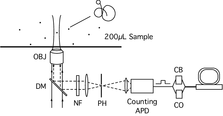
The experimental setup (Fig.2) is an inverted confocal microscopy arrangement. The sample is illuminated by the 514.5nm line of a Ar+ laser (Lexel 85) focused through a 60x water immersion objective (numerical aperature 1.2, Olympus). Incident power was empirically optimized at 100$\mu$W, so that the photon counts per aggregate were at least 50,000 cps, while avoiding significant population of the triplet state or bleaching. Emitted photons are collected through the same objective, directed through a high-pass dichroic mirror (Omega Optical) and a notch filter (Kaiser Optical) to reduce collection of on-axis elastically scattered photons. The collection volume is further refined by focusing the light onto a 25$\mu$m pinhole, eliminating off angle scattering as well as spatially defining the collection volume. The collection volume was empirically determined though the number of molecules measured through FCS as a function of increasing concentration. All FCS measurements were 10 minutes in duration using a ALV 5000 E board for data collection and in-house data analysis software for fitting. The overall detection efficiency of the setup is estimated to be  3 percent. Photons are detected by a counting avalanche photodiode (EG&G/Perkin Elmer), pulsewidth  25ns whose signal is processed by task specific counting board (NI-TIO 6602 National Instruments), controlled by LabVIEW. The period between each photon is measured by counting the number of external clock (4MHz) pulses(source) between each photon pulse (gate). $2^{16}$ photons are collected for each trial. Data acquisition technology limited the total collection time to 1-2s, depending on the incident intensity. Afterpulsing artifacts from the photodiodes were measured $\sim$ 100ns, with comparison to cross-correlation of the same signal in two perpendicular detectors. Digital filtering was used to subtract the afterpulsing noise from the final histogram statistics. DNA concentrations are $\sim$nM in PBS buffer such that only one monomer molecule at any time is within the collection volume.

Photon counting data is collected as fluorescent particles diffuse through the sample volume. When the particles are outside the volume they are dark and undetectable. As they enter the volume they are excited with a certain probability and emit a temporal pattern of photons that are detected by a counter. Given a long integration time, many particles diffuse through the volume producing temporal fluctuations in fluorescence. Whereas the autocorrelation function reveals the timescale of these fluorescence fluctuations, the probability distribution characterizes their amplitude.

Photon counting data was collected for two systems, and the time delay histogram constructed for each (Fig 3). Both samples consist of very dilute (nM) identical sequences of ssDNA in buffer, and observations were made at room temperature ( 25 ^∘C). We consider these systems noninteracting. In the first sample, specifically single end-labeled ssDNA was diluted to an average concentration of 1 molecule per collection beam volume at any time. The number of molecules was calculated from calibration of the collection volume (see Methods) at $100\mu W$ incident power (0.35$\mu m^{3}$). The second sample contained the same sequence ssDNA however tagged with two fluorophores per object (one at each end). This sample was then diluted so that the average intensity in time of the two samples were equal. If the dimer system was exactly twice the fluorescence of the monomer, then the dimer concentration should be 0.5 that of the monomer for the same given intensity. However, due to local quenching effects of the fluorophore, the average concentration of double-dyed molecules in the beam at any time was calculated to be 0.7 to maintain the same intensity. The empirical volume of the beam was calibrated from a serial dilution of a standard dye solution, and the rate of emitted photons per fluor,$\lambda$, measured. $1/\lambda=1/60kHz$. Concentrations of single/double fluorescent aggregates in the beam were 1 and 0.7 molecules respectively.

Empirical measurements demonstrated the quenching could be minimized by hybridization of the ssDNA to a non-fluorescent target. Hybridization of such a short segment (below the persistent length of dsDNA) forces the two fluorophores farther apart, minimizing dye-dye interaction. However, double-dyed molecules never demonstrated a full factor of 2 increase in fluorescence over their single-dyed conterparts. We suspect local quenching interaction of the fluor with the nearby base of the target strand.

The characteristic diffusion time through the sampling volume was extracted from the decay of the autocorrelation function. Due to the resolution of our correlator software $(10^{-8}s-10^{-2}s)$, we are most sensitive to the diffusion across the short axis of the beam profile. Hence, the characteristic time extracted from time correlation of the data is most representative of $\tau_{\perp}$. Through FCS measurements, we find that $\tau_{\perp}\simeq 300\mu$s for both single-dyed molecules and double-dyed molecules, Using a random walk simulation and a geometical approximation for the long axis of the beam profile, we estimate $\tau_{\|}$ to be $100\tau_{\bot}$.

In all theoretical curves of the figures below, we use $\lambda=60$kHz for specific brightness of the single-dyed molecules and an enhancement of $1/0.7\simeq 1.4\lambda$ for the double-dyed molecules, The transverse diffusion time $\tau_{\perp}=300\mu$ s is substituted into the theoretical formula for for both single-dyed and double-dyed molecules.

At first glance, the two distributions of Fig.3 are completely indistinguishable. However upon closer examination it is possible to see the two curves slowly diverge at large $\Delta t$ with the double dye data falls slightly above the single dye data. The comparison between the analytical expression of the time delay histograms with large and small $\Delta t$ approximations (5.20) and (5.21) is shown in Fig.4, where the ratio of the experimental histogram to the theoretical one is plotted versus the time delay $\Delta t$. It is evident that the formula (5.19) together with the approximation (5.17), denoted as $\rho_{\rm{theory}}(\Delta t)$ in the Figures, is robust for single (A) and double dyed (C) samples. (B) and (D) are exploded views of the small $\Delta t$ domain of each histogram. The curve labeled by “linear” or “quadratic” corresponds to the theoretical formula (5.21) with terms beyond linear or quadratic truncated. The quality of the agreement is improved from the linear truncation to the quadratic truncation. The curve labeled by “Poisson” corresponds to $\rho_{\rm theor.}(\Delta t)$ given by a Poissonian, i.e. $\ln\rho_{\rm theor.}(\Delta t)=\ln\rho_{\rm theor.}(0)-\lambda\Delta t$, which is clearly a poor description of the experimental histogram.

Although these simulations successfully differentiate the two systems, the analysis is somewhat cumbersome. A common mathematical technique to highlight the subtle differences in distributions is moment analysis. Similar techniques have proven useful in fluctuation spectroscopy [14, 15, 16]. The first moment is the mean, the second moment the standard deviation, the third the skewness, etc.

Returning to Fig.3, we note a profound difference between the experimental data and a single Poissonian process. The straight lines represent two hypothetical single Poission systems with different timescales. For the simple detection of emitted photons within a fixed volume one might expect the statistics to resemble a single Poissonian process. [17] However, when the particles are allowed to diffuse through the boundaries of the volume, an additional Poissonian process contributes to the overall photon statistics. [18, 19] Not only must we account for the stochastic nature of the emission process, we must also consider the number distribution of aggregates passing into the beam volume from the larger sample reservoir. The statistics of the time series of the photon counting can be highlighted through Mandel’s Q parameter (Eqn 2.5) introduced in section II.

We develop the binning moment as a complementary technique to FIMDA. In FIMDA [11] each histogram is representative of the number count distribution using a certain binning window size. For every change in binning window size, a new histogram is constructed. Likewise, every histogram has its own unique set of moments. All first moments should be equal to the product of the average intensity and the the window size and will not show any difference between the two systems (single dye and double dye) in accordance with the experimental procedure described in the first paragraph of this section. Starting with the second moment, the difference between the two system emerges. In Fig 5, we plot the second moment normalized according to (2.5) for both system and the corresponding theoretical curve given by (5.13). The data for the two systems are clearly distinguishable and agree well with the theoretical prediction.

If the photon histogram were a single Poissonian, all correlations as well as the Q parameter would vanish. Therefore the correlation functions and the Q parameter measure the deviation of the photon histogram from a Poissonian. Recall that the time-delay histogram is essentially the result of a two Poissonian processes. If we re-examine Fig 3 (although it is a time delay, not number counting histogram) and focus on the dashed line through the short $\Delta t$ domain, divergence from the single Poisson increases as $\Delta t$ increases. For binning windows smaller than the diffusion time, the statistics are primarily due to the intrinsic fluorescence of the fluorophore. Since both systems contain 2 fluors, the two distributions vary little in this domain. At longer times, each molecule samples the inhomogeneous beam profile as it diffuses. Hence the diffusion dependent statistics dominate the long time domain and are responsible for the notably different Q parameters of the samples.

In traditional fluorescence correlation spectroscopy, triplet state effects and various quenching processes are the principal mechanisms that overshadow structural information. To parse out these contributions, one may need to explore the higher binning moments than have been examined in this work. Our mathematical formulation provides the complete systematics for this purpose. Such secondary effects introduce additional timescales to the problem (not simply the fluorescence rate and the diffusion time to cross the collection volume discussed in this paper). Also, some details of the electronic transition inside a fluorophore should be addressed. This modeling can be achieved by enlarging the quantum mechanical analog with a multi-component wave function $\psi_{i}$ and a matrix Hamiltonian

where

Each component of the wave function, $\psi_{i}$ represents the probability of a DNA molecule at a particular spatial location with its fluorophore in the $i$-th electronic level and $W_{ij}$ the transition rates from $i$th $\to$ $j$th of electronic levels.

In principle, such an elaboration should also be implemented in the absence of triplet state effects and quenching processes, since the fluorescence rate combines the excitation rate from the ground state and the spontaneous emission rate from the excitation levels. For two electronic levels with ’0’ labeling the ground state and ’1’ the excitation state, we have $W_{01}=\lambda u(\vec{r})$ and $W_{10}=\lambda_{s}$, Einstein’s $A$-coefficient. The Schroedinger equation (4.18) is split into two components:

The approximation employed in previous sections amounts to $\lambda_{s}>>\lambda$ and $\lambda>>1/\tau_{\perp}$, the diffusion time. In this case, the spontaneous emission is almost instantaneous once the fluorophore is excited and the second equation, (7.4), gives rise to $\lambda_{s}\psi_{1}\simeq\lambda u\psi_{0}$ at equilibrium. Substituting it back (7.3), we obtain (4.18) with $h$ given by (4.14). For the experimental data presented in this paper, a 60kHz photon time delay histogram at 3% detection efficiency, the excitation rate is 60/3%=2MHz, and the corresponding fluorescence time is 500ns, much longer than the typical spontaneous emission time, 10ns. Our approximation is therefore adequate.

We have developed a mathematical formulation to analyze the time delay series of fluorescence photons from diffusing particles, based on a probability generating functional and its quantum mechanical analog. Although it may appear formal, since some analytical expressions such as the auto-correlation function have been obtained by less sophisticated means, the approach is systematic. The potential of this general approach will be realized when dealing with systems of greater complexity, e.g. in the presence of the chemical reaction discussed below.

We have designed an experiment to differentiate fluorescent aggregates in solution. ssDNA monomers are labeled with a single fluorophore and dimers with two fluorophores. Secondary effects such as chemical reactions, triplet state effects and various quenching processes have been neglected in our model. However these effects have been minimized by using dilute solutions to avoid self-interaction and Rhodamine 6G, a fluorophore with little triplet state at low incident intensities.

Although we have only addressed ideal experimental conditions of the non-reacting case in this manuscript, typical biological/chemical systems react (aggregation or cooperative binding). Our technique can be modified to include these reactions. One must generalize the quantum mechanical analog to the case with several species of particles, each representing a fluorescence molecule, interacting with each other. Without going to technical details which will be reported elsewhere, we quote the generalization of our formulation analog in the presence of a binary reaction,

The Hamiltonian of the quantum mechanical analog in (4.12) is given by

where

and

and the generating functional is no longer factorizable. In this Halmitonian, the pairs of operators ($\psi$,$\bar{\psi}$) or ($\phi$,$\bar{\phi}$) are the creation/annihilation operators of a molecule of species A or B. $D_{A(B)}$ and $\lambda_{A(B)}$ are the diffusion constant and the specific brightness of the species A(B). The first term of the reaction part, $H_{\rm chem}$ represents the creation of a B-molecule, the second term represents the creation of a pair of A-molecules, the third term signifies the annihilation of a pair of A-molecules and the last term signifies the annihilation of a B-molecule. The function $\sigma(\vec{R}|\vec{r},\vec{r}^{\prime})$ or $\sigma^{\prime}(\vec{r},\vec{r}^{\prime}|\vec{R})$ denotes the reaction rate in each direction of (8.1). In physics, the Hamiltonian (8.2) describes a system of interacting bosons of two species. The equilibrium state of the fluorescence-diffusion-reaction process will be analogous to the ground state which carries a Bose condensate. The proportion of each species in the condensate is determined by the mass-action law and the fluctuations are calculatable with well developed field theoretic method. In terms of the generating functional (4.2) and the functional derivative (4.4), we are able to calculate various correlation functions of the photon counting histogram in the presence of chemical reactions using techniques developed in quantum field theory. This approach is expected to be more systematic than the conventional reaction kinetics.

The works of N.L. Goddard, G. Bonnet and A. Libchaber are supported in part by Mathers Foundation and the Burrough-Welcome Fund. The work of H. C. Ren is supported in part by US Department of Energy under the contract DE-FG02-91ER40651-TASK B. We would also like to thank David Mauzerall for his discussions and suggestions.

To derive the $\Delta t$ distribution (the distribution function of the time interval between two successive photon emissions), we start with the case with finite time bins ($\epsilon$ is sufficiently small that the probability of more than one photons within a bin can be ignored.) and look for the probability of one photon event in $n^{th}$-bin, one photon event in $(n+l)^{th}$ bin with $\Delta t=(l-1)\epsilon$ and no photon in the bins between them. Up to a normalization constant, the probability is

By summing over $n$ with a fixed $l$, we find the probability of successive $l-1$ empty bins

Taking the limit of infinitesimal bins, i.e., $\epsilon\to 0$ at fixed $T$ and $\Delta t$, we obtain the desired distribution function (4.7).

Consider the case of a single time bin, i.e.${\cal N}=1$, we have

and

Under the assumption that each photon counting by the detector is statistically independent of others, the probability of detecting $m$ photons out of $n$ incident photons is

with $\eta$ the detector efficiency. Therefore

References

- [1] L.Mandel, Opt.Lett.4, 205(1979).
- [2] D.Magde, E.L.Elson, and W.W.Webb Phys.Rev.Lett. 29,704-8(1972).
- [3] G. Bonnet, O. Krichevsky, and A. Libchaber Proc. Nat. Acad. Sci. USA 95, 8602(1998).
- [4] E.L. Elson and D. Magde Biopolymers 13, 1-27(1974).
- [5] C.R.Cantor and P.R.Schimmel Biophysical Chemistry : Techniques for the Study of Structure and Function, Vol II (1980).
- [6] H.Scher and E.W.Montroll Phys.Rev. B 12, 2455 (1975).
- [7] Y.Chen, J.D.Müller, P.T.C.So and E.Gratton Biophys.J. 77, 553-567 (1999).
- [8] P.Kask, K.Palo, D.Ulmann, and K.Gall Proc. Nat. Acad. Sci. USA 96, 13756-13761(1999).
- [9] E.Novikov and N.Boens J.Chem.Phys. 114, 1745-1753(2001).
- [10] P.Schwille, F.J. Meyer-Almes, and R.Rigler Biophys.J 72, 1878-1886 (1997).
- [11] K.Palo, Ü.Mets, S.Jäger, P.Kask, and K.Gall Biophys.J 79, 2858-2866 (2000).
- [12] Rigler, R., U. Mets, J. Widengren, and P. Kask Eur.Biophys.J 22 69-175(1993).
- [13] P.Kask, K.Palo, N.Fay, L.Brand, Ü.Mets, D.Ullmann, J.Jungmann, J.Pschorr, and K.Gall Biophys.J 78, 1703-1713 (2000).
- [14] A.G.Palmer and N.L.Thompson, Biophys.J 52, 257-270(1987).
- [15] H.Qian and E.L.Elson Proc. Nat. Acad. Sci. USA 87, 5479-5483 (1990).
- [16] H.Qian and E.L.Elson Biophys.J 57, 374-380 (1990).
- [17] L.Mandel, Proc.Phys.Soc. 72, 1037-1048(1958).
- [18] D.L.Snyder Random Point Processes. Wiley-Interscience, New York (1975).
- [19] L.Mandel and E.Wolf Optical Coherence and Quantum Optics. Cambridge Univ. Press, Cambridge (1995).
- [20] J.Enderlein Phys. Lett. A 6, 427-433 (1996).
- [21] R. P. Feynman and A. Q. Hibbs Quantum Mechanics and Path Integrals. McGraw-Hill Book Co, New York (1965).