Simulation of seismic response in a city-like environment

A noticeable feature of many earthquake-prone cities such as Mexico-City [1], [2], [3], Nice [4], Los Angeles [5]  etc., is that they are partially or wholly built on soft soil. Seismogram records in such cities indicate amplification of the ground motion, beating phenomena, long codas and substantial spatial variability of response.

To analyze the possible causes of these puzzling effects, we study the action of a seismic wave on a relatively-simple structural model with both geological and man-made features. Our 2D model has three components, as in [6], (from bottom to top in Fig. 1): a hard half space (HHS), overlain by a soft dissipative soil layer (SL), in which are partially imbedded a set of even softer dissipative blocks (SB). HHS and SL are geological features, the set of SB, which are homogenized for purpose of the analysis, is man-made and constitutes the visible component of an idealized city.

Real media disperse and attenuate waves. In [6], all the material components of the ’city’ were taken to be lossless. In order to obtain a more realistic picture of wave propagation in the soft layer and in the homogenized blocks, we consider them to be composed of dissipative media. We follow the approach exposed in [7], [8], [9] and show how it can be used to simulate SH viscoelastic wave propagation.

Even when the media are dissipative, we find that the presence of the blocks gives rise to ground motion amplification, beating phenomena, long duration and spatial variability of response, which are not present in the case of a flat ground (i.e., without homogenized blocks) for the same solicitation. We also find that these effects are similar, although with less amplitude, to those for non-dissipative media (as assumed in [6]).

In order to understand, identify, and quantify some causes of these features, we study the influence of the distance separating the homogenized blocks. If the homogenized blocks are considered to be homogenized buildings, we show that decreasing the distance between buildings increases the interaction between buildings, and between buildings and the soft layer, but does not modify fundamentally the response in terms of amplification and duration. We attribute duration effects to the excitation of Love-like modes due essentially to the presence of the blocks [10], [11].

Referring once again to Fig. 1, the blocks of the city are assumed to be in welded contact with the substratum by an interface on which we assume (as in [6]) the continuity of displacement and normal stress. Our “city” is invariant in the $x_{3}$-direction with $x_{1}$, $x_{2}$, $x_{3}$ being the cartesian coordinates, and $x_{2}$ increasing with the depth (see Fig.1 wherein the sagittal plane is displayed). The support of the seismic source is a line in the $x_{3}$-direction, and is located deep in the HHS, radiating a Ricker pulse cylindrical shear-horizontal (SH) displacement field. Only the $x_{3}$-component of this field is non-vanishing and invariant with respect to $x_{3}$, so that the total field underneath and on the free surface is also SH-polarized and invariant with respect to $x_{3}$. The resulting problem is 2D with the displacement field depending only on $x_{1}$, $x_{2}$ and on time $t$.

We denote by $h_{i}$, $w_{i}$ and $d_{i,i+1}^{j}$, the height, width of the block $B_{i}$ and space interval between the blocks $B_{i}$ and $B_{i+1}$ for the three configurations, $C^{j}~;~j=1,2,3$, we studied. The substratum $\Omega_{0}$ is occupied by a linear, isotropic, medium $M_{0}$, characterized by mass density $\rho(\mathbf{x})=\rho_{0}$, shear modulus $\mu(\mathbf{x})=\mu_{0}$, and quality factor $Q(\mathbf{x})=Q_{0}=+\infty$, with $\mathbf{x}=(x_{1},x_{2})$. The soft layer $\Omega_{1}$ is occupied by a linear, isotropic, dissipative medium $M_{1}$ characterized by mass density $\rho(\mathbf{x})=\rho_{1}$, relaxed shear modulus $\mu_{R}(\mathbf{x})=\mu_{R1}$, and quality factor $Q(\mathbf{x})=Q_{1}$. The blocks $\Omega_{2}$ are occupied by the linear, isotropic, dissipative medium $M_{2}$ characterized by mass density $\rho(\mathbf{x})=\rho_{2}$, relaxed shear modulus $\mu_{R}(\mathbf{x})=\mu_{R2}$, and quality factor $Q(\mathbf{x})=Q_{2}$.

Since problems in seismology are essentially concerned with transient phenomena it is natural to treat them in the space-time rather than the space-frequency framework. This also presents certain advantages from the numerical point of view. The obvious approach is then to solve the second-order-in-time wave equation (Navier equation when the medium is isotropic) for the displacement vector. A less-obvious, but numerically-advantageous method [12], [13], [14], is to cast the wave equation into the form of two first-order-in-time partial differential equations, for the two unknowns constituted by the displacement and pseudo-velocity vectors.

In the following, we show briefly (more details are given in [7], [8], [9]) how to do this for motion in viscoelastic, isotropic media. Since our problem relates to 2D, SH motion, the unknowns reduce to the single non-zero component of the displacement vector and the two components of a pseudo-velocity vector. We show that these unknowns satisfy two coupled first-order-in-time partial differential equations, in which appear a set of unknowns (usually called memory variables) whose existence is due to the viscoelastic nature of the media. Each of these coefficients is shown to satisfy a first-order-in-time partial differential equation whose driving term is related to the pseudo-velocity vector.

In an isotropic, non pre-stressed, elastic ( viscoelastic) medium $M$, the stress tensor $s_{kl}$ is related to the strain tensor $e_{kl}$ by the Hooke-Cauchy constitutive relation

$$s_{kl}=\lambda\delta_{kl}e_{mm}+2\mu e_{kl}~~;~~k,l=1,2,3~.$$

(1)

wherein the Einstein summation convention is implicit, $\delta_{kl}$ is the Kronecker delta and $e_{kl}$ is related to the particle displacement vector (whose elements are $u_{k}$) by

$$e_{kl}=\frac{1}{2}\left(u_{k,l}+u_{l,k}\right)~,$$

(2)

with $u_{k,l}$ signifying the partial derivative of $u_{k}$ with respect to the $l$-th cartesian coordinate $x_{l}$. Furthermore, $\lambda$ is the bulk modulus and $\mu$ the rigidity. In elastic media, $\lambda$ and $\mu$ are, at most, functions of position, whereas in viscoelastic media (i.e., with memory),  $\mu$ depends also on time.

The tensorial wave equation in elastic and viscoelastic media, in the context of linear (visco) elasticity, is

$$s_{kl,k}-\rho\partial_{t}^{2}u_{l}=-\rho f_{l}~~;~~k,l=1,2,3~,$$

(3)

wherein $\rho$ is the mass density of the medium, $f_{l}$ the $l$-th component of the applied force density vector, $t$ the time variable and $\partial_{t}^{2}:=\frac{\partial^{2}}{\partial t^{2}}$. This set of partial differential equations can be recognized to be linear in terms of the displacement $u_{l}$ since $s_{kl}$ is a linear function of $u_{l}$.

The 2D SH aspect of the problem is encompassed in the assumptions: $f_{1}=f_{2}=0$, $u_{1}=u_{2}=0$ and $u_{3,3}=0$. so that the tensorial wave equation becomes

$$(s_{13,1}+s_{23,2})-\rho\partial_{t}^{2}u_{3}=-\rho f_{3}~.$$

(4)

Let

$$\boldsymbol{\sigma}:=(s_{13},s_{23})~~,~~u:=u_{3}~~,~~f:=f_{3}~.$$

(5)

Then

$$\boldsymbol{\sigma}=(\mu u_{3,1},\mu u_{3,2})=\mu\nabla u~,$$

(6)

which is the expression of the constitutive relation for the situation corresponding to that of 2D SH motion in (visco)elastic media.

By the same token, the wave equation for 2D SH motion in isotropic, non pre-stressed, (visco)elastic media becomes

$$\nabla\cdot(\mu\nabla u)-\rho\partial_{t}^{2}u=-\rho f~,$$

(7)

which is of the general form

$$\nabla\cdot(a\nabla U)-b\partial_{t}^{2}U+cF=0~.$$

(8)

We are able to show that this equation can be obtained from the two first-order-in-time equations

$$-\partial_{t}\mathbf{V}+a\nabla{U}=0~,$$

(9)

$$b\partial_{t}U-\nabla\cdot\mathbf{V}=cG~.$$

(10)

by taking the divergence of (9), the partial time derivative of (10), and subtracting the equations so obtained. This leads to (8) provided $G$ is chosen so that

$$F=\partial_{t}G~.$$

(11)

Thus, instead of being confronted with solving a single, second-order-in-time partial differential equation for $U$, we must solve two first-order-in-time partial differential equations for the displacement $U$ and the pseudo-velocity $\mathbf{V}$.

By a viscoelastic solid we mean a material whose rigidity at an instant $t$ depends on the whole strain history of the solid, so that the Hooke-Cauchy relation takes the more general (convolution) form (for 2D, SH motion)

$$\boldsymbol{\sigma}(\mathbf{x},t)=\int_{-\infty}^{t}\mu(\mathbf{x},t-\tau)\nabla u(\mathbf{x},\tau)d\tau~,$$

(12)

wherein $\mathbf{x}:=(x_{1},x_{2})$. When the constitutive relation (12) is inserted into the wave equation, the latter becomes an integro-differential equation which is very cumbersome to solve numerically because it requires saving in memory the whole history of the solution at all points of the compuational domain. To overcome this inconvenience, Emmerich and Korn [15] propose a (essentially Maxwell body) method whereby they approximate the Fourier spectrum $\mu(\mathbf{x},\omega)$ (with $\omega$ the angular frequency) of the viscoelastic rigidity modulus $\mu(\mathbf{x},t)$ by a rational function of frequency.

Consider $\mathcal{F}(\mathbf{x},t)$ to be a function of $\mathbf{x}$ and $t$; then $\mathcal{F}(\mathbf{x},\omega)$ is its Fourier spectrum (with $\omega$ the angular frequency) such that

$$\mathcal{F}(\mathbf{x},t)=\int_{-\infty}^{\infty}\mathcal{F}(\mathbf{x},\omega)\exp(-i\omega t)d\omega~.$$

(13)

Consequently, the frequency domain constitutive relation corresponding to (12) is

$$\boldsymbol{\sigma}(\mathbf{x},\omega)=\mu(\mathbf{x},\omega)\nabla u(\mathbf{x},\omega)~.$$

(14)

We suppose that the spectrum function $\mu(\mathbf{x},\omega)$ is known (from experimental data) and wish to approximate it in the rational function manner. To do this, we introduce the relaxation function $R(\mathbf{x},t)$ defined by

$$\mu(\mathbf{x},t)=\frac{dR(\mathbf{x},t)}{dt}~.$$

(15)

This relaxation function is assumed in [15] to take the form of a discrete sum of sinusoidal functions

$$R(\mathbf{x},t)\approx\mu_{R}(\mathbf{x})\left[1+\frac{\delta\mu(\mathbf{x})}{\mu_{R}(\mathbf{x})}\sum_{j=1}^{J}a_{j}(\mathbf{x})\exp(-\omega_{j}t)\right]H(t)~,$$

(16)

wherein $J$ is some integer, preferably not too large to reduce the computational effort, $H(t)$ is the Heaviside function, $\mu_{R}(\mathbf{x})$ the relaxed rigidity modulus (equal to the time-invariant rigidity in the elastic case), $\delta\mu(\mathbf{x})$ a differential rigidity which is a measure of the departure from elasticity, $\omega_{j}$ the relaxation frequencies, it being understood that the coefficients $a_{j}$ obey the (normalization) relation

$$\sum_{j=1}^{J}a_{j}(\mathbf{x})=1~.$$

(17)

From (15)-(17)we find

$$\mu(\mathbf{x},\omega)\approx\mu_{R}(\mathbf{x})\left[1+\sum_{j=1}^{J}y_{j}(\mathbf{x})\frac{i\omega}{i\omega-\omega_{j}}\right]~,$$

(18)

wherein

$$y_{j}(\mathbf{x}):=\frac{\delta\mu(\mathbf{x})}{\mu_{R}(\mathbf{x})}a_{j}(\mathbf{x})~.$$

(19)

In the works of Emmerich and Korn [15] and Groby and Tsogka [7], [8], [9] the weight functions $\{y_{j}(\mathbf{x}~;~j=1,2,..,J)\}$ are determined in unique manner from a given $\mu(\mathbf{x},\omega)$ by solving an overdetermined linear system arising from sampling $(\ref{3.10})$ at a set of relaxation frequencies $\omega_{l}$ which are chosen equidistant on a logarithmic scale in the interval $\left[\omega_{max}/100,\omega_{max}\right]$, with $\omega_{max}$ the maximal frequency of the solicitation spectrum.

We introduce the new variables $\boldsymbol{\zeta}_{j}(\mathbf{x},\omega)$:

$$\boldsymbol{\zeta}_{j}(\mathbf{x},\omega):=\frac{i\omega}{i\omega-\omega_{j}}y_{j}(\mathbf{x})\mu_{R}(\mathbf{x})\nabla u(\mathbf{x},\omega)~,$$

(20)

so that

$$\boldsymbol{\sigma}(\mathbf{x},t)=\mu_{R}\nabla u(\mathbf{x},t)+\sum_{j=1}^{J}\boldsymbol{\zeta}_{j}(\mathbf{x},t)=\boldsymbol{\sigma}_{R}(\mathbf{x},t)+\sum_{j=1}^{J}\boldsymbol{\zeta}_{j}(\mathbf{x},t)~.$$

(21)

It is then straightforward to show that $\boldsymbol{\zeta}_{j}$ satisfies the differential equation:

$$\partial_{t}\boldsymbol{\zeta}_{j}(\mathbf{x},t)+\omega_{j}\boldsymbol{\zeta}_{j}(\mathbf{x},t)=y_{j}(\mathbf{x})\partial_{t}\boldsymbol{\sigma}_{R}(\mathbf{x},t)~.$$

(22)

We now introduce a new function $\eta_{j}(\mathbf{x},t)$ such that

$$\rho(\mathbf{x})\partial_{t}^{2}\eta_{j}(\mathbf{x},t):=\nabla\cdot\boldsymbol{\zeta}_{j}(\mathbf{x},t)~.$$

(23)

Then, it can be shown that:

$$\partial_{t}^{2}\eta_{j}(\mathbf{x},t)+\omega_{j}\partial_{t}\eta_{j}(\mathbf{x},t)=\frac{1}{\rho(\mathbf{x})}\nabla\cdot\left(y_{j}(\mathbf{x})\mu_{R}(\mathbf{x})\nabla u(\mathbf{x},t)\right)~,$$

(24)

$$\nabla\cdot\left(\mu_{R}(\mathbf{x})\nabla u(\mathbf{x},t)\right)+\rho(\mathbf{x})\sum_{j=1}^{J}\partial_{t}^{2}\eta_{j}(\mathbf{x},t)-\rho(\mathbf{x})\partial_{t}^{2}u(\mathbf{x},t)+\rho(\mathbf{x})f(\mathbf{x},t)=0~.$$

(25)

The latter equation is of the form (8) provided we make the associations: $U=u$, $a=\mu_{R}$, $b=\rho$, $F=f+\sum_{j=1}\partial_{t}^{2}\eta_{j}$, and $c=\rho$, so that employing the previously-demonstrated equivalence between (8) and a system of two first-order-in-time partial differential equations, we find, at present, that (25) is equivalent to the couple of equations:

$$\mu_{R}(\mathbf{x})\nabla u(\mathbf{x},t)-\partial_{t}\mathbf{V}(\mathbf{x},t)=0~,$$

(26)

$$\rho\partial_{t}u(\mathbf{x},t)-\nabla\cdot\mathbf{V}(\mathbf{x},t)=\rho g(\mathbf{x},t)+\sum_{j=1}^{J}\partial_{t}\eta_{j}(\mathbf{x},t)~,$$

(27)

wherein $g$ is such that

$$\partial_{t}g(\mathbf{x},t)=f(\mathbf{x},t)~.$$

(28)

The last step is to introduce (26) into (24) followed by integration over $t$ and neglect of the integration constant:

$$\partial_{t}\eta_{j}(\mathbf{x},t)+\omega_{j}\eta_{j}(\mathbf{x},t)=\frac{1}{\rho(\mathbf{x})}\nabla\cdot\left(y_{j}(\mathbf{x})\mathbf{V}(\mathbf{x},t)\right)~.$$

(29)

Our procedure for solving a problem of 2D SH wave motion, in response to the solicitation $f(\mathbf{x},t)$, in the temporal interval $[0,T]$ and spatial domain $\Omega$, occupied by a isotropic, viscoelastic medium $M$ characterized by the density $\rho(\mathbf{x})$ and rigidity spectrum function $\mu(\mathbf{x},\omega)$, thus boils down to:

• •

  obtain $g(\mathbf{x},t)$ from $f(\mathbf{x},t)$ via

  $$\partial_{t}g(\mathbf{x},t)=f(\mathbf{x},t)~~;~~\mathbf{x}\in\Omega~,~t\in[0,T]~,$$

  (30)

• •

  obtain the weight functions $y_{j}(\mathbf{x})$ from $Q:=\Re(\mu(\mathbf{x},\omega))/\Im(\mu(\mathbf{x},\omega))$ via

  $$\mu(\mathbf{x},\omega)=\mu_{R}(\mathbf{x})\left[1+\sum_{j=1}^{J}y_{j}(\mathbf{x})\frac{i\omega}{i\omega-\omega_{j}}\right]~~;~~\mathbf{x}\in\Omega~,~\omega\in\left[\frac{\omega_{max}}{100},\omega_{max}\right]~,$$

  (31)

• •

  solve the coupled system of three first-order-in-time partial differential equations

  $$\mu_{R}(\mathbf{x})\nabla u(\mathbf{x},t)-\partial_{t}\mathbf{V}(\mathbf{x},t)=0~~;~~\mathbf{x}\in\Omega~,~t\in[0,T]~,$$

  (32)

  $$\rho\partial_{t}u(\mathbf{x},t)-\nabla\cdot\mathbf{V}(\mathbf{x},t)=\rho g(\mathbf{x},t)+\sum_{j=1}\partial_{t}\eta_{j}(\mathbf{x},t)~~;~~\mathbf{x}\in\Omega~,~t\in[0,T]~,$$

  (33)

  $$\partial_{t}\eta_{j}(\mathbf{x},t)+\omega_{j}\eta_{j}(\mathbf{x},t)=\frac{1}{\rho(\mathbf{x})}\nabla\cdot\left(y_{j}(\mathbf{x})\mathbf{V}(\mathbf{x},t)\right)~~;~~\mathbf{x}\in\Omega~,~t\in[0,T]~,$$

  (34)

  for  the  three  unknown   functions   $u(\mathbf{x},t)$,  $\mathbf{V}(\mathbf{x},t)$,   and   $\boldsymbol{\eta}:=\{\eta_{j}(\mathbf{x},t)~;~j=1,2,..,J\}$.

The aim of this work was first to prove that amplification, beatings, long duration, and spatial variability of response are observed even when the media (in the layer and blocks) are dissipative, and that essentially the same phenomena are involved in both the dissipative and non-dissipative cases.

The snapshot of the modulus of the total displacement field in Fig. 3 pertains to the case in which there are no blocks in the city, for the dissipative layer case. As mentioned in [10], [6], [18], one does not expect the Love modes to be excited to any great extent when the source is far from the layer. This is what is actually observed in Fig. 3 since the displacement field in the soft layer is not typical of that of a Love mode.

Fig. 4 depicts the snapshot for a city overlying a dissipative layer with ten blocks. One observes a series of hot spots inside the low-velocity layer, constituting an indication of something like a standing wave in the layer betraying the excitation of a quasi-Love mode [11], [4], [18]. This configuration also gives rise to rather large response in the blocks and on the ground, as was previously observed in [6] for non-dissipative media, and in [10] for a periodic distribution of identical blocks.

The time records and spectra, presented in Figs. 5-8 call for the following comments.

• •

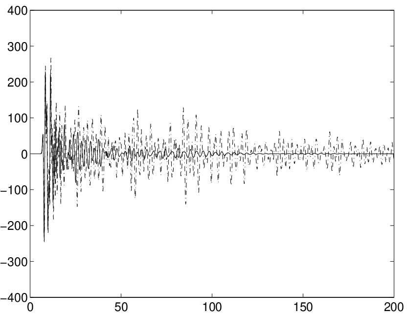
  Fig. 5 exhibits the time history of the velocity at the summit of building no. 6, for both the dissipative and non-dissipative cases. The durations are much longer when there is no dissipation. Nevertheless, in the dissipative case, beatings are observed and the duration of motion is of the order of 2 min.

• •

  Fig. 6 contains the time histories of the velocity, and the velocity spectra at the summits and on the ground in between blocks for city $C^{1}$.

• •

  Fig. 7 contains the time histories of the velocity, and the velocity spectra at the summits and on the ground in between blocks for city $C^{2}$.

• •

  Fig. 8 contains the time histories of the velocity, and the velocity spectra at the summits and on the ground in between blocks for city $C^{3}$.

The results in terms of the vulnerability indices are given in Table 2.

This work was initiated in [6], in which the authors considered the soft layer and blocks to be occupied by non-dissipative media.

The time histories in Figs. 6-8 herein, relative to dissipative blocks and a dissipative soft layer, again exhibit amplification, beating phenomena, long codas and spatial variability of response in all three cities. The spectra exhibit so-called ’splittings’ [10], which are responsible for beating phenomena and part of the duration. The durations (time during the which amplitude is more than $0.1$ of the maximal amplitude) are not notably different for the three cities (i.e., maximal duration of around $120s$) for the three configurations. The entries in Table 2 indicate that the vulnerability indices of the blocks are significantly-large even in the case of dissipative media. The spectra are more irregular (i.e., the number of peaks is larger) when the average separation of the blocks is smaller. This may constitute an indication of greater structure-soil-structure and/or greater block-to-block interaction responsible for more efficient excitation of quasi Love modes (these are neither the rigid base block modes, nor the Love modes in the absence of the buildings, but a combination of the two [11]).

The traditional [1], [2] (and even quite recent [3], [5], [4]) choice, concerning the analysis of earthquakes in cities built on soft soil as Nice and Mexico City, has been to introduce complexity into the substratum while leaving the free surface flat or with large-scale topographic features [4]. The buildings are not included in such models and their response is treated separately, if at all, using the flat ground motion as the input. This has led to response predictions that are more in line with what has actually been observed during tremors in a variety of cities (Nice, Los Angeles, Mexico City, etc.). Nevertheless, one or several of the features, namely duration, peak velocities and spatial variability, of observed response, differ from those of the predictions. This is possibly due to the fact that the fine structure of the substratum is usually unknown. Another plausible hypothesis is that small-scale irregularities on the free surface and on interface between the foundations and the soft soil, introduced by the existence of buildings in a city, may contribute significantly to the overall motion of the site.

This hypothesis was shown to be tenable for: i) a non-dissipative basement underlying a city of ten, non-equispaced, non-equally sized, homogenized, non-dissipative blocks in [6], and ii) a dissipative basement underlying a city with an infinite number of equispaced, identical, dissipative blocks in [10]. Herein, we again considered cities with ten non-equispaced non-equally sized, homogenized blocks, but the latter, as well as the underlying layer, were considered to be dissipative.

We found that the introduction of dissipation does not eliminate the previously-found anomalous effects arising from the presence of the blocks, which take the form of peak ground and block motion amplifications, beatings, and long codas. As expected, the durations turned out to be smaller than in the non-dissipative case, but the vulnerability indices remained significantly large. When the spacing between blocks was reduced, we found some evidence of increased structure-soil-structure and block-to-block interactions, but, contrary to expectation, this did not have significant effects on either the duration of motion or on the peak amplification.

These anomalous effects, as well as their spatial variability, are qualitatively the same as those observed in Mexico City and underline the fact that the individual buildings or groups of buildings (blocks) play a very active role in the overall motion of a city submitted to a seismic disturbance.

In the future, it will be necessary to examine to what extent the anomalous response is affected by the location and type of seismic source, as well as by the duration of the pulse radiated from this source (note that studies such as [3], [18] take no account of the buildings of the city).

References

- [1] Bard P.-Y., Eeri M., Campillo M., Chávez-Garcia F.J., and Sanchez-Sesma F.J. The Mexico earthquake of Spetember 19, 1985-a theoretical inverstigation fo large-and small-scale amplification effects in th eMexico City valley. Earthquake Spectra, 4:609–633, 1988.
- [2] Chávez-Garcia F.J. and Bard P.-Y. Site effects in Mexico City eight yers after the Spetemeber 1985 Michoacan erathquakes. Soil Dynam.Earthquek Engrg., 13:229–247, 1994.
- [3] Faeh D., Suhadolc P., Mueller S., and Panza G.F. A hybrid method for the estimation of ground motion in sedimentary basins: quantitative modeling of Mexico City. Bull.Seism.Soc.Am., 84:383–399, 1994.
- [4] Semblat J.-F., Duval A.-M. and Dangla P. Numerical analysis of seismic wave amplification in Nice (France) and comparisons with experiments. Soil Dynam.Earthquek Engrg., 19:347–362, 2000.
- [5] Olsen K.B. Site amplification in the Los Angeles basin from three-dimensional modeling of ground motion. Bull.Seism.Soc.Am., 90:99–94, 2000.
- [6] Tsogka C. and Wirgin A. Simulation of seismic response in an idealized city. Soil Dynam.Earthquek Engrg., 23:391–402, 2003.
- [7] Groby J.-P. and Tsogka C. A time domain method for modeling wave propagation phenomena in viscoacoustic media. In Cohen G.C. and Heikkola E., editors, Mathematical and Numerical Aspects of Wave Propagation, pages 911–915. Springer, 2003.
- [8] Groby J.-P. Tsogka C. and Wirgin A. A time domain method for modeling viscoelastic SH wave propagtion in a city-like environment. In Doolin D. Kammerer A. Nogami T. Seed R.D. and Towhata I., editors, Proceedings of the 11th Inetrnational Conference on Soil Dynamics & Earthquake Engineering, pages 887–894. University of California and Stallion Press, 2004.
- [9] Groby J.-P. and Tsogka C. A time domain method for modeling viscoacoustic wave propagation. ArXiv, math.NA/0403297, 2004.
- [10] Wirgin A. and Bard P.-Y. Effects of buildings on the duration and amplitude of ground motion in Mexico City. Bull.Seism.Soc.Am., 86:914–920, 1996.
- [11] Wirgin A. and Kouoh-Bille L. Amplification du mouvement du sol au voisinage d’un groupe de montagne de profile rectangulaire ou triangulaire soumis à une onde sismique SH. In Génie Parasismique et Aspects Vibratoire dans le Génie Civil, pages ES28–ES37. AFPS, 1993.
- [12] Bécache E., Joly P., and Tsogka C. Application of the fictitious domain method to 2D linear elastodynamic problems. J.Comput.Acoust., 9:1175–1202, 2001.
- [13] Bécache E., Joly P., and Tsogka C. An analysis of new mixed finite elements for the approximation of wave propagation problems. SIAM J.Numer.Anal., 37:1053–1084, 2000.
- [14] Tsogka C. Modélisation mathématique et numérique de la propagation des ondes élastique tridimensionnelles dans des milieux fissurés. PhD thesis, University Paris IX, 2000.
- [15] Emmerich H. and Korn M. Incorporation of Attenuation into time-domain computations of seismic wave fields. Geophys., 52:1252–1264, 1987.
- [16] Collino F. and Tsogka C. Applications of th ePML absorbing layer model to the linear elastodynamic problem in anisutropic heteregeneous media. Geophys., 66:294–305, 2001.
- [17] Kjartansson E. Constant Q wave propagation and attenuation. J.Geophys.Res., 84:4737–4748, 1979.
- [18] Groby J.-P. and Wirgin A. 2D ground motion at a soft viscoelastic layer/hard substratum site in response to SH cylindrical seismic waves radiated by deep and shallow line sources. ArXiv, physics/04010907, 2004.