PhysicsGP: A Genetic Programming Approach to Event Selection
Abstract
We present a novel multivariate classification technique based on Genetic Programming. The technique is distinct from Genetic Algorithms and offers several advantages compared to Neural Networks and Support Vector Machines. The technique optimizes a set of human-readable classifiers with respect to some user-defined performance measure. We calculate the Vapnik-Chervonenkis dimension of this class of learning machines and consider a practical example: the search for the Standard Model Higgs Boson at the LHC. The resulting classifier is very fast to evaluate, human-readable, and easily portable. The software may be downloaded at: http://cern.ch/cranmer/PhysicsGP.html
Keywords:
Genetic Programming, Triggering, Classification, VC Dimension, Genetic Algorithms, Neural Networks, Support Vector Machines1 Introduction
The use of multivariate algorithms in the search for particles in High Energy Physics has become quite common. Traditionally, a search can be viewed from a classification point of view: from a tuple of physical measurements (i.e., momenta, energy, etc.) we wish to classify an event as signal or background. Typically, this classification is realized through a Boolean expression or cut designed by hand. The high dimensionality of the data makes this problem difficult in general and favors more sophisticated multivariate algorithms such as Neural Networks, Fisher Discriminants, Kernel Estimation Techniques, or Support Vector Machines. This paper focuses on a Genetic Programming approach and considers a specific example: the search for the Higgs Boson at the LHC.
The use of Genetic Programming for classification is fairly limited; however, it can be traced to the early works on the subject by Koza koza:gp. More recently, Kishore et al. extended Koza’s work to the multicategory problem kishore:2000. To the best of the authors’ knowledge, the work presented in this paper is the first use of Genetic Programming within High Energy Physics.
In Section 2 we provide a brief history of evolutionary computation and distinguish between Genetic Algorithms (GAs) and Genetic Programming (GP). We describe our algorithm in detail for an abstract performance measure in Section 3 and discuss several specific performance measures in Section 4.
Close attention is paid to the performance measure in order to leverage recent work applying the various results of statistical learning theory in the context of new particle searches. This recent work consists of two components. In the first, the Neyman-Pearson theory is translated into the Risk formalism Cranmer:Acta; Cranmer:2003vu. The second component requires calculating the Vapnik-Chervonenkis dimension for the learning machine of interest. In Section 5, we calculate the Vapnik-Chervonenkis dimension for our Genetic Programming approach.
Because evolution is an operation on a population, GP has some statistical considerations not found in other multivariate algorithms. In Section 6 we consider the main statistical issues and present some guiding principles for population size based on the user-defined performance measure.
Finally, in Section 7 we examine the application of our algorithm to the search for the Higgs Boson at the LHC.
2 Evolutionary Computation
In Genetic Programming (GP), a group of ‘‘individuals’’ evolve and compete against each other with respect to some performance measure. The individuals represent potential solutions to the problem at hand, and evolution is the mechanism by which the algorithm optimizes the population. The performance measure is a mapping that assigns a fitness value to each individual. GP can be thought of as a Monte Carlo sampling of a very high dimensional search space, where the sampling is related to the fitness evaluated in the previous generation. The sampling is not ergodic -- each generation is related to the previous generations -- and intrinsically takes advantage of stochastic perturbations to avoid local extrema11 1 These are the properties that give power to Markov Chain Monte Carlo techniques..
Genetic Programming is similar to, but distinct from Genetic Algorithms (GAs), though both methods are based on a similar evolutionary metaphor. GAs evolve a bit string which typically encodes parameters to a pre-existing program, function, or class of cuts, while GP directly evolves the programs or functions. For example, Field and Kanev Field:1997kt used Genetic Algorithms to optimize the lower- and upper-bounds for six 1-dimensional cuts on Modified Fox-Wolfram “shape” variables. In that case, the phase-space region was a pre-defined 6-cube and the GA was simply evolving the parameters for the upper and lower bounds. On the other hand, our algorithm is not constrained to a pre-defined shape or parametric form. Instead, our GP approach is concerned directly with the construction and optimization of a nontrivial phase space region with respect to some user-defined performance measure.
In this framework, particular attention is given to the performance measure. The primary interest in the search for a new particle is hypothesis testing, and the most relevant measures of performance are the expected statistical significance (usually reported in Gaussian sigmas) or limit setting potential. The different performance measures will be discussed in Section 4, but consider a concrete example: , where and are the number of signal and background events satisfying the event selection, respectively.
3 The Genetic Programming Approach
While the literature is replete with uses of Genetic Programming and Genetic Algorithms, direct evolution of cuts appears to be novel. In the case at hand, the individuals are composed of simple arithmetic expressions, , on the input variables . Without loss of generality, the cuts are always of the form . By scaling, , and translation, , of these expressions, single- and double-sided cuts can be produced. An individual may consist of one or more such cuts combined by the Boolean conjunction AND. Fig. 1 shows the signal and background distributions of four expressions that make up the most fit individual in a development trial.
Due to computational considerations, several structural changes have been made to the naïve implementation. First, an Island Model of parallelization has been implemented (see Section 3.5). Secondly, individuals’ fitness can be evaluated on a randomly chosen sub-sample of the training data, thus reducing the computational requirements at the cost of statistical variability. There are several statistical considerations which are discussed in Section 6.

3.1 Individual Structure, Mutation, and Crossover
The genotype of an individual is a collection of expression trees similar to abstract syntax trees that might be generated by a compiler as an intermediate representation of a computer program. An example of such a tree is shown in Fig. 2a which corresponds to a cut . Leafs are either constants or one of the input variables. Nodes are simple arithmetic operators: addition, subtraction, multiplication, and safe division22 2 Safe division is used to avoid division by zero..When an individual is presented with an event, each expression tree is evaluated to produce a number. If all these numbers lie within the range , the event is considered signal. Otherwise the event is classified as background.

Initial trees are built using the PTC1 algorithm described in luke00two. After each generation, the trees are modified by mutation and crossover. Mutation comes in two flavors. In the first, a randomly chosen expression in an individual is scaled or translated by a random amount. In the second kind of mutation, a randomly chosen subtree of a randomly chosen expression is replaced with a randomly generated expression tree using the same algorithm that is used to build the initial trees.
While mutation plays an important rôle in maintaining genetic diversity in the population, most new individuals in a particular generation result from crossover. The crossover operation takes two individuals, selects a random subtree from a random expression from each, and exchanges the two. This process is illustrated in Fig. 2.
3.2 Recentering
Some expression trees, having been generated randomly, may prove to be useless since the range of their expressions over the domain of their inputs lies well outside the interval for every input event. When an individual classifies all events in the same way (signal or background), each of its expressions is translated to the origin for some randomly chosen event exemplar , viz. . This modification is similar to, and thus reduces the need for, normalizing input variables.
3.3 Fitness Evaluation
Fitness evaluation consumes the majority of time in the execution of the algorithm. So, for speed, the fitness evaluation is done in C. Each individual is capable of expressing itself as a fragment of C code. These fragments are pieced together by the Python program, written to a file, and compiled. After linking with the training vectors, the program is run and the results communicated back to the Python program using standard output.
The component that serializes the population to C and reads the results back from the generated C program is configurable, so that a user-defined performance measure may be implemented.
3.4 Evolution & Selection Pressure
After a given generation of individuals has been constructed and the individuals’ fitnesses evaluated, a new generation must be constructed. Some individuals survive into the new generation, and some new individuals are created by mutation or crossover. In both cases, the population must be sampled randomly. To mimic evolution, some selection pressure must be placed on the individuals for them to improve. This selection pressure is implemented with a simple Monte Carlo algorithm and controlled by a parameter . The procedure is illustrated in Fig. 3. In a standard Monte Carlo algorithm, a uniform variate is generated and transformed into the variable of interest by the inverse of its cumulative distribution. Using the cumulative distribution of the fitness will exactly reproduce the population without selection pressure; however, this sampling can be biased with a simple transformation. The right plot of Fig. 3 shows a uniform variate being transformed into , which is then inverted (left plot) to select an individual with a given fitness. As the parameter grows, the individuals with high fitness are selected increasingly often.
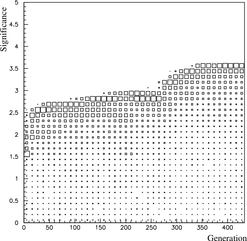
While the selection pressure mechanism helps the system evolve, it comes at the expense of genetic diversity. If the selection pressure is too high, the population will quickly converge on the most fit individual. The lack of genetic diversity slows evolutionary progress. This behavior can be identified easily by looking at plots such as Fig. 4. We have found that a moderate selection pressure has the best results.

3.5 Parallelization and the Island Model
GP is highly concurrent, since different individuals’ fitness evaluations are unrelated to each other, and dividing the total population into a number of sub-populations is a simple way to parallelize a GP problem. Even though this is a trivial modification to the program, it has been shown that such coarse grained parallelization can yield greater-than-linear speedup david95parallel. Our system uses a number of Islands connected to a Monitor in a star topology. CORBA is used to allow the Islands, which are distributed over multiple processors, to communicate with the Monitor.
Islands use the Monitor to exchange particularly fit individuals each generation. Since a separate monitor process exists, a synchronous exchange of individuals is not necessary. The islands are virtually connected to each other (via the Monitor) in a ring topology.
4 Performance Measures
The Genetic Programming approach outlined in the previous section is a very general algorithm for producing individuals with high fitness, and it allows one to factorize the definition of fitness from the algorithm. In this section we examine the function(al) which assigns each individual its fitness: the performance measure.
Before proceeding, it is worthwhile to compare GP to popular multivariate algorithms such as Support Vector Machines and Neural Networks. Support Vector Machines typically try to minimize the risk of misclassification , where is the target output (usually 0 or -1 for background and 1 for signal) and is the classification of the input. This is slightly different than the error function that most Neural Networks with backpropagation attempt to minimize: Werbos; PDP1. In both cases, this performance measure is usually hard-coded into a highly optimized algorithm and cannot be easily replaced. Furthermore, these two choices are not always the most appropriate for High Energy Physics, as will be discussed in Section 4.1.
The most common performance measure for a particle search is the Gaussian significance, , which measures the statistical significance (in “sigmas”) of the presence of a new signal. The performance measure is calculated by determining how many signal events, , and background events, , a given individual will select in a given amount of data (usually measured in fb-1).
The is actually an approximation of the Poisson significance, , the probability that an expected background rate will fluctuate to . The key difference between the two is that as , the Poisson significance will always approach 0, but the Gaussian significance may diverge. Hence, the Gaussian significance may lead to highly fit individuals that accept almost no signal or background events.
The next level of sophistication in significance calculation is to include systematic error in the background only prediction . These calculations tend to be more difficult and the field has not adopted a standard Cousins:1992qz; Cranmer:2003vt; Linnemann:2003vw. It is also quite common to improve the statistical significance of an analysis by including a discriminating variable FinalLHWG:2003sz.
In contrast, one may be more interested in excluding some proposed particle. In that case, one may wish to optimize the exclusion potential. The exclusion potential and discovery potential of a search are related, and G. Punzi has suggested a performance measure which takes this into account quite naturally Punzi.
Ideally, one would use as a performance measure the same procedure that will be used to quote the results of the experiment. For instance, there is no reason (other than speed) that one could not include discriminating variables and systematic error in the optimization procedure (in fact, the authors have done both).
4.1 Direct vs. Indirect Methods
Certain approaches to multivariate analysis leverage the many powerful theorems of statistics, assuming one can explicitly refer to the joint probability density of the input variables and target values . This dependence places a great deal of stress on the asymptotic ability to estimate from a finite set of samples . There are many such techniques for estimating a multivariate density function given the samples Scott; Cranmer:2000du. Unfortunately, for high dimensional domains, the number of samples needed to enjoy the asymptotic properties grows very rapidly; this is known as the curse of dimensionality.
Formally, the statistical goal of a new particle search is to minimize the rate of Type II error. This is logically distinct from, but asymptotically equivalent to, approximating the likelihood ratio. In the case of no interference between the signal and background, this is logically distinct from, but asymptotically equivalent to, approximating the signal-to-background ratio. In fact, most multivariate algorithms are concerned with approximating an auxiliary function that is one-to-one with the likelihood ratio. Because the methods are not directly concerned with minimizing the rate of Type II error, they should be considered indirect methods. Furthermore, the asymptotic equivalence breaks down in most applications, and the indirect methods are no longer optimal. Neural Networks, Kernel Estimation techniques, and Support Vector Machines all represent indirect solutions to the search for new particles. The Genetic Programming approach is a direct method concerned with optimizing a user-defined performance measure.
5 Statistical Learning Theory
In 1979, Vapnik provided a remarkable family of bounds relating the performance of a learning machine and its generalization capacity Vapnik:1979. The capacity, or Vapnik-Chervonenkis dimension (VCD) is a property of a set of functions, or learning machines, , where is a set of parameters for the learning machine Vapnik:1968.
In the two-class pattern recognition case considered in this paper, an event is classified by a learning machine such that . Given a set of events each represented by , there are possible permutations of them belonging to the class signal or background. If for each permutation there exists a member of the set which correctly classifies each event, then we say the set of points is shattered by that set of functions. The VCD for a set of functions is defined as the maximum number of points which can be shattered by . If the VCD is , it does not mean that every set of points can be shattered, but that there exists some set of points which can be shattered. For example, a hyperplane in can shatter points (see Fig. 5 for ).

In the modern theory of machine learning, the performance of a learning machine is usually cast in the more pessimistic setting of risk. In general, the risk, , of a learning machine is written as
| (1) |
where measures some notion of loss between and the target value . For example, when classifying events, the risk of mis-classification is given by Eq. 1 with . Similarly, for regression tasks one takes . Most of the classic applications of learning machines can be cast into this formalism; however, searches for new particles place some strain on the notion of risk Cranmer:Acta; Cranmer:2003vu.
The starting point for statistical learning theory is to accept that we might not know in any analytic or numerical form. This is, indeed, the case for particle physics, because only can be obtained from the Monte Carlo convolution of a well-known theoretical prediction and complex numerical description of the detector. In this case, the learning problem is based entirely on the training samples with elements. The risk functional is thus replaced by the empirical risk functional
| (2) |
There is a surprising result that the true risk can be bounded independent of the distribution . In particular, for
| (3) | |||||
where is the VC dimension and is the probability that the bound is violated. As , , or the bound becomes trivial. The second term of the right hand side is often referred to as the VC confidence – for , , and the VC confidence is about 12%.
While the existence of the bounds found in Eq. 3 are impressive, they are frequently irrelevant. In particular, for Support Vector Machines with radial basis functions for kernels the VCD is formally infinite and there is no bound on the true risk. Similarly, for Support Vector Machines with polynomial kernels of degree and data embedded in dimensions, the VCD is which grows very quickly.
This motivates a calculation of the VCD of the GP approach.
5.1 VCD for Genetic Programming
The VC dimension, , is a property of a fully specified learning machine. It is meaningless to calculate the VCD for GP in general; however, it is sensible if we pick a particular genotype. For the slightly simplified genotype which only uses the binary operations of addition, subtraction, and multiplication, all expressions are polynomials on the input variables. It has been shown that for learning machines which form a vector space over their parameters,33 3 A learning machine, , is a vector space if for any two functions and real numbers the function . Polynomials satisfy these conditions. the VCD is given by the dimensionality of the span of their parameters Sontag. Because the Genetic Programming approach mentioned is actually a conjunction of many such cuts, one also must use the theorem that the VCD for Boolean conjunctions, , among learning machines is given by , where is a constant Sontag.
If we placed no bound on the size of the program, arbitrarily large polynomials could be formed and the VCD would be infinite. However, by placing a bound on either the size of the program or the degree of the polynomial, we can calculate a sensible VCD. The remaining step necessary to calculate the VCD of the polynomial Genetic Programming approach is a combinatorial problem: for programs of length , what is the maximum number of linearly independent polynomial coefficients? Fig. 6 illustrates that the smallest program with nine linearly independent coefficients requires eight additions, eighteen multiplications, eighteen variable leafs, and nine constant leafs for a total of 53 nodes. A small Python script was written to generalize this calculation.
The Genetic Programming approach with polynomial expressions has a relatively small VCDs (in our tests with seven variables nothing more than was found) which affords the relevance of the upper-bound proposed by Vapnik.
5.2 VCD of Neural Networks
In order to apply Eq. 3, one must determine the VC dimension of Neural Networks. This is a difficult problem in combinatorics and geometry aided by algebraic techniques. Eduardo Sontag has an excellent review of these techniques and shows that the VCD of neural networks can, thus far, only be bounded fairly weakly Sontag. In particular, if we define as the number of weights and biases in the network, then the best bounds are . In a typical particle physics neural network one can expect , which translates into a VCD as high as , which implies for reasonable bounds on the risk. These bounds imply enormous numbers of training samples when compared to a typical training sample of . Sontag goes on to show that these shattered sets are incredibly special and that the set of all shattered sets of cardinality greater than is measure zero in general. Thus, perhaps a more relevant notion of the VCD of a neural network is given by .
6 Statistical Fluctuations in the Fitness Evaluation
In this section we examine the trade-off between the time necessary to evaluate the fitness of an individual and the accuracy of the fitness when evaluated on a finite sample of events. Holding computing resources fixed, the two limiting cases are:
- 1
With very large sample sizes, one can expect excellent estimation of the fitness of individuals and a clear “winner” at the expense of very little mutation and poorly optimized individuals.
- 2
With very small sample sizes, one can expect many mutations leading to individuals with very high fitness which do not perform as reported on larger samples.
Illustrated in Fig. 7 is the distribution of fitness for a given “winning” individual generated with a large ensemble of training samples each with 400 events. The fitness reported in the last generation of the training phase (indicated with an arrow) is much higher than the mean of this distribution. In fact, the probability to have randomly chosen a sample of 400 events which would produce such a high empirical significance is about 0.1%.
While the chance that an arbitrary individual’s fitness evaluates several standard deviations from the mean is quite small, with thousands, maybe millions, of individual programs the chance that one will fluctuate significantly can be quite large. Furthermore, the winning individual has a much higher chance of a significant upward fluctuation, because individuals with upward fluctuations have a higher chance of being the winner.
Having recognized that statistical fluctuations in the fitness evaluation complicate matters, we have developed a few guiding principles for reliable use of the algorithm.
- •
For training, the standard deviation of the fitness distribution evaluated on events should be on the order of a noticeable and marginal improvement in the fitness based on the users performance measure.
- •
Select the winning individual with a large testing sample.

If we take as our measure of performance , then it is possible to calculate the variance due to the fluctuations in and . The expected error is given by the standard propagation of errors formula. In particular,
| (4) |
where and via standard rate calculations and and similarly via binomial statistics. For the analysis presented in Section 7, the selection efficiency for signal and background are and , respectively. The predicted rate of signal and background events are , and , respectively. Using these values, one can expect a 10% (5%) relative error on the fitness evaluation with a sample of (400) events. Analogous calculations can be made for any performance measure (though they may require numerical studies) to determine a reasonable sample size. The rule of thumb that relative errors scale as is probably reasonable in most cases.
7 Case Study: The Search for the Higgs Boson at the LHC
Finally we consider a practical example: the search for the Higgs boson at the LHC. While there are many channels available, the recent Vector Boson Fusion analyses offer a sufficiently complicated final state to warrant the use of multivariate algorithms.
The Higgs at the LHC is produced predominantly via gluon-gluon fusion. For Higgs masses such that the second dominant process is Vector Boson Fusion. The lowest order Feynman diagram of the production of Higgs via VBF is depicted in Fig 8. The decay channel chosen is . These channels will also be referred to as , , and , respectively.
These analyses were performed at the parton level and indicated that this process could be the most powerful discovery mode at the LHC in the range of the Higgs mass, , pr_160_113004. These analyses were studied specifically in the ATLAS environment using a fast simulation of the detector ATLFAST. Two traditional cut analyses, one for a broad mass range and one optimized for a low-mass Higgs, were developed and documented in references UW-LowMass-VBF and SciNote. We present results from previous studies without systematic errors on the dominant background included.
In order to demonstrate the potential for multivariate algorithms, a Neural Network analysis was performed UW-nn-VBF. The approach in the Neural Network study was to present a multivariate analysis comparable to the cut analysis presented in UW-LowMass-VBF. Thus, the analysis was restricted to kinematic variables which were used or can be derived from the variables used in the cut analysis.
The variables used were:
- •
- the pseudorapidity difference between the two leptons,
- •
- the azimuthal angle difference between the two leptons,
- •
- the invariant mass of the two leptons,
- •
- the pseudorapidity difference between the two tagging jets,
- •
- the azimuthal angle difference between the two tagging jets,
- •
- the invariant mass of the two tagging jets, and
- •
- the transverse mass.


In total, three multivariate analyses were performed:
- •
a Neural Network analysis using backpropagation with momentum,
- •
a Support Vector Regression analysis using Radial Basis Functions, and
- •
a Genetic Programming analysis using the software described in this Communication.
The Neural Network (NN) analysis is well documented in reference
UW-nn-VBF. The analysis were performed with both the Stutgart
Neural Network Simulator (SNNS)44
4
SNNS can be found here:
www-ra.informatik.uni-tuebingen.de and MLPfit55
5
MLPfit
can be found here:
cern.ch/˜schwind/MLPfit.html with a
7-10-10-1 architecture.
For the Support Vector Regression (SVR) analysis, the BSVM-2.066
6
BSVM can be found here:
www.csie.ntu.edu/˜cjlin/bsvm library was used.
The only parameters are the cost parameter, set to , and the kernel function. BSVM does not support weighted events, so an “unweighted” signal and background sample was used for training.
Because the trained machine only depends on a small subset of “Support Vectors”, performance is fairly stable after only a thousand or so training samples. In this case, 2000 signal and 2000 background training events were used.
Both NN and SVR methods produce a function which characterizes the signal-likeness of an event. A separate procedure is used to find the optimal cut on this function which optimizes the performance measure (in this case the Poisson signficance, ). Fig. 9 shows the distribution of the SVR (left) and NN (right) output values. The optimal cut for the SVR technique is shown as a vertical arrow.
Tab. 1 compares the Poisson significance, , for a set of reference cuts, a set of cuts specifically optimized for low-mass Higgs, Neural Networks, Genetic Programming, and Support Vector Regression. It is very pleasing to see that the multivariate techniques achieve similar results. Each of the methods has its own set of advantages and disadvantages, but taken together the methods are quite complementary.
| Ref. Cuts | low- Opt. Cuts | NN | GP | SVR | |
|---|---|---|---|---|---|
| 120 | 0.87 | 1.25 | 1.72 | 1.66 | 1.44 |
| 120 | 2.30 | 2.97 | 3.92 | 3.60 | 3.33 |
| 120 | 1.16 | 1.71 | 2.28 | 2.26 | 2.08 |
| Combined | 2.97 | 3.91 | 4.98 | 4.57 | 4.26 |
| 130 | 4.94 | 6.14 | 7.55 | 7.22 | 6.59 |
8 Conclusions
We have presented an implementation of a Genetic Programming system specifically applied to the search for new particles. In our approach a group of individuals competes with respect to a user-defined performance measure. The genotype we have chosen consists of Boolean conjunctions of simple arithmetic expressions of the input variables required to lie in the interval . Our implementation includes an island model of parallelization and a recentering algorithm to dramatically improve performance. We have emphasized the importance of the performance measure and decoupled fitness evaluation from the optimization component of the algorithm. We have touched on the relationship of Statistical Learning Theory and VC dimension to the search for new particles and multivariate analysis in general. Finally, we have demonstrated that this method has similar performance to Neural Networks (the de facto multivariate analysis of High Energy Physics) and Support Vector Regression. We believe that this technique’s most relevant advantages are
- •
the ability to provide a user-defined performance measure specifically suited to the problem at hand,
- •
the speed with which the resulting individual / cut can be evaluated,
- •
the fundamentally important ability to inspect the resulting cut, and
- •
the relatively low VC dimension which implies the method needs only a relatively small training sample.
9 Acknowledgments
This work was supported by a graduate research fellowship from the National Science Foundation and US Department of Energy Grant DE-FG0295-ER40896.
References
- (1) J.R. Koza. Genetic Programming: On the Programming of Computers by Means of Natural Selection. MIT Press, Cambridge, MA, 1992.
- (2) J.K. Kishore et. al. Application of genetic programming for multicategory pattern classification. IEEE Transactions on Evolutionary Computation, 4 no.3, 2000.
- (3) K. Cranmer. Multivariate analysis and the search for new particles. Acta Physica Polonica B, 34:6049–6069, 2003.
- (4) K. Cranmer. Multivariate analysis from a statistical point of view. In PhyStat2003, 2003. physics/0310110.
- (5) R. D. Field and Y. A. Kanev. Using collider event topology in the search for the six-jet decay of top quark antiquark pairs. hep-ph/9801318, 1997.
- (6) S. Luke. Two fast tree-creation algorithms for genetic programming. IEEE Transactions on Evolutionary Computation, 2000.
- (7) D. Andre and J.R. Koza. Parallel genetic programming on a network of transputers. In Justinian P. Rosca, editor, Proceedings of the Workshop on Genetic Programming: From Theory to Real-World Applications, pages 111–120, Tahoe City, California, USA, 9 1995.
- (8) P.J. Werbos. The Roots of Backpropagation. John Wiley & Sons., New York, 1974.
- (9) D.E. Rumelhart et. al. Parallel Distributed Processing Explorations in the Microstructure of Cognition. The MIT Press, Cambridge, 1986.
- (10) R.D. Cousins and V.L. Highland. Incorporating systematic uncertainties into an upper limit. Nucl. Instrum. Meth., A320:331–335, 1992.
- (11) K. Cranmer. Frequentist hypothesis testing with background uncertainty. In PhyStat2003, 2003. physics/0310108.
- (12) J. T. Linnemann. Measures of significance in HEP and astrophysics. In PhyStat2003, 2003. physics/0312059.
- (13) Search for the standard model Higgs boson at LEP. Phys. Lett., B565:61–75, 2003.
- (14) G. Punzi. Sensitivity of searches for new signals and its optimization. In PhyStat2003, 2003. physics/0308063.
- (15) D. Scott. Multivariate Density Estimation: Theory, Practice, and Visualization. John Wiley and Sons Inc., 1992.
- (16) K. Cranmer. Kernel estimation in high-energy physics. Comput. Phys. Commun., 136:198–207, 2001.
- (17) V. Vapnik. Estimation of dependences based on empirical data. Nauka, 1979. in Russian.
- (18) V. Vapnik and A.J. Chervonenkis. The uniform convergence of frequencies of the appearance of events to their probabilities. Dokl. Akad. Nauk SSSR, 1968. in Russian.
- (19) E. Sontag. VC dimension of neural networks. In C.M. Bishop, editor, Neural Networks and Machine Learning, pages 69–95, Berlin, 1998. Springer-Verlag.
- (20) D. Rainwater and D. Zeppenfeld. Observing in weak boson fusion with dual forward jet tagging at the CERN LHC. D60:113004, 1999.
- (21) D. Froidevaux E. Richter-Was and L. Poggioli. Atlfast2.0 a fast simulation package for atlas. ATLAS Internal Note ATL-PHYS-98-131.
- (22) K. Cranmer et. al. Search for Higgs bosons decay for using vector boson fusion. ATLAS note ATL-PHYS-2003-002 (2002).
- (23) S. Asai et. al. Prospects for the search of a standard model Higgs boson in ATLAS using vector boson fusion. to appear in EPJ. ATLAS Scientific Note ATL-PHYS-2003-005 (2002).
- (24) K. Cranmer et. al. Neural network based search for Higgs bosons decay for . ATLAS note ATL-PHYS-2003-007 (2002).