2D ground motion at a soft viscoelastic layer/hard substratum site in response to SH cylindrical seismic waves radiated by deep and shallow line sources

Jean-Philippe Groby Thanks: Laboratoire de Mécanique et d’Acoustique, UPR 7051 du CNRS, 31 chemin Joseph Aiguier, 13402 Marseille cedex 20, France, (groby@lma.cnrs-mrs.fr) Armand Wirgin Thanks: LMA/CNRS, 31 chemin Joseph Aiguier, 13402 Marseille cedex 20, France, (wirgin@lma.cnrs-mrs.fr)

August 11, 2026

Abstract

We show, essentially by theoretical means, that for a site with the chosen simple geometry and mechanical properties (horizontal, homogeneous, soft viscoelastic layer of infinite lateral extent overlying, and in welded contact with, a homogeneous, hard elastic substratum of half-infinite radial extent, shear-horizontal motion): 1) coupling to Love modes is all the weaker the farther the seismic source (modeled as a line, assumed to lie in the substratum) is from the lower boundary of the soft layer, 2) for a line source close to the lower boundary of the soft layer, the ground response is characterized by possible beating phenomena, and is of significantly-longer duration than for excitation by cylindrical waves radiated by deep sources. Numerical applications of the theory show, for instance, that a line source, located 40m below the lower boundary of a 60m thick soft layer in a hypothetical Mexico City-like site, radiating a SH pulse of 4s duration, produces substantial ground motion during 200s, with marked beating, at an epicentral distance of 3km. This response is in some respects similar to that observed in real cities located at soft-soil sites so that the model employed herein may help to establish the causes and pinpoint the major contributing factors of the devastating effects of earthquakes in such cities.

Keywords: site response, regional path effects, source position, Love modes, interference maxima, duration, beatings.

Abbreviated title: Seismic site response: a canonical problem

Corresponding author: Armand Wirgin, tel.: 33 4 91 16 40 50, fax: 33 4 91 22 08 75, e-mail: wirgin@lma.cnrs-mrs.fr

1 Introduction

This investigation is relevant to several topics of broad interest in seismic wave propagation:

(a) regional path effects in connection with seismic response in urban environments [1], [2], [3], [4], [5], [6], [7], [8], [9], [10]

(b) effects of the underlying soil heterogeneities, lateral variations of the underlying soil layer, and built environment on seismic ground response at various (particularly urban) sites [11], [12], [13], [6], [14], [15], [16], [17],[18], [9], [10], [19]

(c) analysis of surface wave response on the ground to determine the structure and composition of the crust [11] and underground fault zones [20], [21]

(d) analysis of surface wave response on the ground to identify earthquake sources [22], [23].

Research on topic (a) was rekindled by efforts to explain some puzzling features of the devastating Michoacan earthquake which struck Mexico City in 1985. Other than the fact that the response in downtown Mexico varied considerably in a spatial sense, was quite intense and of very-long duration [24], [25] (as much as $\sim$ 3 min) at certain locations, and often took the form of a quasi-monochromatic signal with beating, a remarkable feature of this earthquake was that such strong (in the sense just mentioned) response could be caused by a seismic disturbance so far (its epicenter was in the subduction zone off the Pacific coast approximately 350 km) from the city [26], [27], [9], [10]. A part of the cause of the large intensity and long-duration was attributed in [2] to multipathing between the source and the site. This hypothesis was further explored in [26], [27] while being associated with surface wave propagation of the Rayleigh and Love types, presumably between the source and the entry to the Mexico City basin, via the intervening crust.

In a rather complete (other than the neglect of attenuation) 3D numerical study [5], the long duration and large amplitude of response at various distances from subduction zone earthquakes in Mexico were attributed to the entrapment of the seismic disturbance in an acccretionary prism (wedge-shaped heterogeneity) of the crust and its subsequent propagation to the point of observation. The authors of this work later [3], [4] stressed the role of higher-order surface waves which propagate in the relatively-high Q layer of the Trans Mexican Volcanic Belt (TMVB) underlying the soft clay basin of Mexico City in addition to that of the accretionary prism in producing large response (particularly with respect to duration) in the city. More recently, an analysis [1] of seismograms recorded at various sites in central Mexico, for earthquake sources located in the subduction zone off the Pacific coast, have shown that the crustal structure (including that of the TMVB, composed of low-velocity volcanic lava and tuff overlying higher velocity limestone) between the source and observation points "acts as a waveguide for surface waves coming from distances greater than 200km", leading, by an unexplained mechanism, to amplification and increase of duration of motion at various sites, this being thought to account for at least part of the anomalous response in Mexico City to remote seismic disturbances. Numerical results obtained in earlier studies (e.g., [9], [10]) with a rather complete, 2D hybrid model of the propagation path between the source and the Mexico-City basin, and of the action of the basin on the incident wave, also stressed the important role of regional path effects on anomalous response.

Anomalous response in other cities such as Beijing, Bucharest, Rome, etc. has been studied in great detail, principally in numerical manner, within the framework of the UNESCO-IGCP project 414 [17], [8]. The features of this response were attributed to the specifics of the source parameters, regional path effects, and the specifics of the soil distribution and geometry in the urban basins (see next paragraph). These findings have been substantiated in a more recent study [18].

Topic (b) deals with a class of alternative or complementary (so-called local) paradigms for explaining seismic motion in urban sites built on soft soil. Even though the anomalous response in 1985 in Mexico City originated in a subduction zone source whose epicentral distance was some 350 km from the city, it has been common to seek explanations of this response (and others such as in Nice [13], [19] and Bucharest [14]) by employing models involving vertically-propagating or nearly vertically-propagating plane waves. This requires that the focal distance of the source to the surface be large and that the epicentral distance from the source to the city be rather small. Although both of these conditions are often not met in practice (and, in particular, as concerns the 1985 Michoacan earthquake), the vertically-propagating plane wave sollicitation usually prevails in the theoretical/numerical studies [14], [7], [28], apparently because it simplifies the analysis (another reason is that it facilitates comparison with the so-called 1D model of normally-incident plane waves on a vertically-layered half space). This has the effect of putting the focus on what occurs in the structure vertically below the city, namely, on the soft basin on which the earthquake-prone cities are built. Thus, a considerable amount of studies (see [26], [29], [28] for comprehensive reviews) examine the (local) effect of the soft basin on the incident wave, but at present, it is thought that local effects account for only part of the anomalous response [26], [27], [17], [8], [1], [18]. Another idea that has been explored in the past few years is that the buildings of the city, in interaction with the soft soil and with each other, may also amplify and lengthen the duration of the ground motion (see [12], [19] for reviews of this subject). All of these studies (including or excluding the buildings) point to the central role of surface waves, qualified either as locally-launched surface (e.g., Love) waves (at the basin edges or at heterogeneities of the soft soil) [30], [29], [9], [18] or as quasi-Love waves (excited at the base of the buildings and re-amplified by interaction with neighboring buildings [12], [31], [19]) as a possible causal agent of anomalous response, but little [32], if any, theoretical evidence has been given to back up these assertions.

Topic (c) is classical in seismological geophysics [33]. The seismic signals associated with various types of surface (e.g., Love and Rayleigh) waves are oft-used tools for reconstructing features of the earth’s crust such as thickness, composition (e.g., vertical layering characteristics [33], [34]) and even lateral heterogeneities [35], [11]. More recently [20], [21], it has been shown that seismic sources in the neighborhood of fault zones (FZ, i.e., soft nearly-vertical layers surrounded by relatively hard soil) excite surface waves (qualified as "trapped") in the vicinity of the FZ which propagate to the ground where they can be detected and used to furnish information on the physical and geometrical characteristics of the FZ. To treat these inverse problems in a fully unambiguous manner requires a thorough understanding of the way the seismic source interacts (notably how accurately one must know the position and characteristics of the source) with the inhomogeneities.

Topic (d) is also a classical one in seismology, the main concern being to localize and qualify (e.g., determine the moment tensor of) earthquake sources [22], [23]. As the seismic wave, including its surface-wave components, travels laterally (sometimes over long distances) in and along the crust before reaching the measurement locations on the ground, the inverse problem is difficult to solve if the crustal features (which can include lateral heterogeneity) are not known beforehand. In any case, it is important to determine the influence of errors of the crustal model on the reconstruction of the source location and moment tensor, and to do this requires an appropriate theoretical analysis.

The theoretical-numerical investigation herein is focused on topics (a) and (b). In contrast to the inverse-scattering topics (c) and (d) (to which our analysis could be applied) wherein the response is known and the propagation medium and/or the source are to be determined, the problem we are faced with herein deals with forward-scattering: given the seismic source and the characteristics of the propagation medium, determine the response (displacement in the frequency and/or time domain) on the ground. More specifically, we shall be concerned with a (deceivingly-) simple canonical scattering problem: that of a cylindrical SH pulse wave impinging on a soft homogeneous layer, the latter being horizontal, of infinite lateral extent, bounded above by the ground and below by an interface with a half space filled with hard homogeneous rock. The questions we address, and that we think can be answered with the help of such a simple model, are:

(i) is it possible to obtain anomalous (in the sense mentioned above in connection with the Michoacan earthquake) response without any lateral heterogeneity (arising from volumic inclusions or uneveness of interfaces) in the underground medium?

(ii) what is the relation of 1D to 2D response and how adequate is it to model the general response of the configuration by its response to a (nearly) vertically-incident plane wave?

(iii) how does the focal distance of the source affect the response?

(iv) how does the epicentral distance affect the response?

(v) how does the contrast of mechanical properties between the layer and the half space affect the ground response?

(vi) how does the thickness of the layer affect the response?

(vii) how do the spectral characteristics of the incident pulse affect the response?

It will be shown that a source radiating cylindrical waves in a fully-elastic soft layer/hard half space medium produces a ground response which is the sum of three terms corresponding to various combinations of two types of waves in the soft layer (SL) and hard half space (HHS):

(1) standing body waves (SBW) in the SL and body waves (BW) in the HHS,

(2) standing body waves in the SL and surface waves (SW) in the HHS,

(3) standing surface waves (SSW) in the SL and surface waves in the HHS.

Only type (2) waves correspond to Love modes (at the resonance frequencies of these modes) and the conditions for optimal excitation and maximal contribution of these modes will be rendered explicit. It will be shown that large-duration (i.e., anomalous) response generally requires a preponderant contribution of at least one (usually the lowest-order) of the Love modes to the overall response. The type (1) waves dominate in the situation in which the focal distance is large and do not usually produce long-duration response, although they can produce strong (although normal) response when the contrast of mechanical properties between the SL and HHS is large. Beating phenomena will be shown to be a consequence of interference between type (1) and type (2) waves which both lead to maxima in response at nearly the same (low) frequency. Type (3) waves turn out to have negligible contribution to overall response. Most of these features carry over to the case in which the layer is lossy. The practical consequences of these results, in relation with topics (a) and (b), will be discussed.

2 Description of the configuration

Fig. 2.1 represents a cross-section (sagittal plane) view of the site. $\Gamma_{g}$ is the ground, assumed to be flat and horizontal, above which is located the air medium, assumed to be the vacumn. $\Omega_{1}$ is the laterally-infinite domain occupied by the mechanically-soft layer and $h$ is its thickness. $\Omega_{0}$ is the semi-infinite domain (substratum) occupied by a mechanically-hard medium, and $\Gamma_{h}$ the flat, horizontal interface between the layer and the substratum. A $Ox_{1}x_{2}x_{3}$ cartesian coordinate system is attached to this configuration such that $O$ is on the ground, $x_{2}$ increases with depth and $x_{3}$ is perpendicular to the (sagittal) plane of the figure. With $\mathbf{i}_{j}$ the unit vector along the positive $x_{j}$ axis, we note that the unit vectors normal to $\Gamma_{g}$ and $\Gamma_{h}$ are $\mathbf{i}_{2}$ . The media filling $\Omega_{0}$ and $\Omega_{1}$ are $M^{0}$ and $M^{1}$ respectively and the latter are assumed to be initially stress-free, linear, isotropic and homogeneous. We assume that $M^{0}$ is non-dissipative and $M^{1}$ is generally (unless specified otherwise) dissipative.

The seismic disturbance is delivered to the site in the form of a shear-horizontal (SH) cylindrical pulse wave radiated by a line source (perpendicular to the sagittal plane) located at $\mathbf{x}^{s}:=(x_{1}^{s},x_{2}^{s})$ , with, by hypothesis, $x_{2}^{s}>h$ (i.e., $\mathbf{x}^{s}\in\Omega_{0}$ ). The SH nature of this wave means that the motion associated with it is strictly transverse (i.e., in the $x_{3}$ direction and independent of the $x_{3}$ coordinate). Both the SH polarization and the invariance of the incident wave with respect to $x_{3}$ are communicated to the fields that are generated at the site in response to the incident wave. Thus, our analysis will deal only with the propagation of 2D SH waves (i.e., waves that depend exclusively on the two cartesian coordinates $x_{1},~x_{2}$ and that are associated with motion in the $x_{3}$ direction only).

We shall be concerned with a description of the elastodynamic wavefield on the ground (i.e., on $\Gamma_{g}$ ) resulting from the cylindrical seismic wave sollicitation of the site.

Refer to caption — Figure 2.1: Cross section view of the configuration.

3 Governing equations

3.1 Space-time domain wave equations

In a generally-inhomogeneous, isotropic elastic or viscoelastic medium $M$ occupying $\mathbb{R}^{3}$ , the time-domain wave equation for SH waves is:

\nabla\cdot(\mu(\mathbf{x},\omega)\nabla u(\mathbf{x},t))-\rho(\mathbf{x})\partial_{t}^{2}u(\mathbf{x},t)=-\rho(\mathbf{x})f(\mathbf{x},t)~,

(3.1)

wherein $u$ is the displacement component in the $\mathbf{i}_{3}$ direction, $f$ the component of applied force density in the $\mathbf{i}_{3}$ direction, $\mu$ the Lamé descriptor of rigidity, $\rho$ the mass density, $t$ the time variable, $\omega$ the angular frequency, $\partial^{n}_{t}$ the $n-$ th partial derivative with respect to $t$ , and $\mathbf{x}=(x_{1},x_{2})$ . Since our configuration involves two homogeneous media and the applied force is assumed to be non-vanishing only in $\Omega_{0}$ , we have

\left(c^{m}(\omega)\right)^{2}\nabla\cdot\nabla u^{m}(\mathbf{x},t)-\partial_{t}^{2}u^{m}(\mathbf{x},t)=-f(\mathbf{x},t)\delta_{m0}~~;~~\mathbf{x}\in\Omega_{m}~,

(3.2)

wherein $m$ superscripts designate the medium (0 for $M^{0}$ or 1 for $M^{1}$ ), $\delta_{m0}=1$ for $m=0$ and equal to zero otherwise, and $c^{m}$ is the generally-complex velocity of shear body waves in $M^{m}$ , related to the density and rigidity by

\left(c^{m}(\omega)\right)^{2}=\frac{\mu^{m}(\omega)}{\rho^{m}}~,

(3.3)

it being understood that $\rho^{m},\mu^{m}(\omega)~;~m=0,1$ are constants with respect to $\mathbf{x}$ .

3.2 Space-time domain representation of the impulsive force

In all that follows we choose the pseudo-Ricker type of impulse line source function

f(\mathbf{x},t)=-\delta(\mathbf{x}-\mathbf{x^{s}})3\frac{\partial}{\partial t}\left[-2\alpha^{2}\left(1-2\alpha^{2}\left(t-t_{0}\right)^{2}\right)e^{-\alpha^{2}\left(t-t_{0}\right)^{2}}\right]=\\ \delta(\mathbf{x}-\mathbf{x^{s}})12\alpha^{4}\left[-3\left(t-t_{0}\right)+2\alpha^{2}\left(t-t_{0}\right)^{3}\right]e^{-\alpha^{2}\left(t-t_{0}\right)^{2}}~,

(3.4)

wherein $\alpha=\pi\nu_{0}$ and $t_{0}=1/\nu_{0}$ and $\delta(~~)$ the Dirac delta distribution.

3.3 Space-frequency domain wave equations

The frequency-domain versions of the wave equations are obtained by expanding the force density and displacement in Fourier integrals:

f(\mathbf{x},t)=\int_{-\infty}^{\infty}f(\mathbf{x},\omega)e^{-i\omega t}d\omega~~,~~u^{m}(\mathbf{x},t)=\int_{-\infty}^{\infty}u^{m}(\mathbf{x},\omega)e^{-i\omega t}d\omega~,\forall t\in\mathbb{R}~,

(3.5)

so as to give rise to the Helmholtz equations

\nabla\cdot\nabla u^{m}(\mathbf{x},\omega)+\left(k^{m}(\omega)\right)^{2}u^{m}(\mathbf{x},\omega)=\\ -f(\mathbf{x},\omega)\delta_{m0}~~;~~\forall\mathbf{x}\in\Omega_{m}~~;~~m=0,1~,

(3.6)

wherein

k^{m}(\omega):=\frac{\omega}{c^{m}(\omega)}=\omega\sqrt{\frac{\rho^{m}}{\mu^{m}(\omega)}}~.

(3.7)

is the generally-complex wavenumber in $M^{m}$ . Actually, due to the assumptions made in sect. 1:

k^{0}(\omega):=\frac{\omega}{c^{0}}=\omega\sqrt{\frac{\rho^{0}}{\mu^{0}}}~,

(3.8)

(i.e., $k^{0}$ is real),

f^{m}(\mathbf{x},\omega)=S(\omega)\delta(\mathbf{x}-\mathbf{x^{s}})~,

(3.9)

wherein $S(\omega)$ is the spectrum of the incident pulse. In fact, the spectrum corresponding to the chosen (see (3.4) pseudo-Ricker impulsive force is

S(\omega)=3\frac{i\omega^{3}}{2\sqrt{\pi}\alpha}e^{i\omega t_{0}-\frac{\omega^{2}}{4\alpha^{2}}}~.

(3.10)

3.4 Material constants in a dissipative medium

A word is now in order about the dissipative nature of the layer. When a medium $M$ is lossy, the wavenumber therein is complex and can be written (omitting, for the moment, the $\omega$ dependence) as

k=k^{\prime}+ik"~,

(3.11)

where, by convention,

\Re k=k^{\prime}\geq 0~~,\Im k=k"\geq 0~.

(3.12)

We now refer to (3.7) and note that complex $k$ implies complex $\mu$ , due to the fact that it is advisable to consider the mass density to be a real quantity. Thus, we write

\mu=\mu^{\prime}-i\mu"~.

(3.13)

In order to retain the positive real aspect of the rigidity for elastic materials, we take

\Re\mu=\mu^{\prime}\geq 0~,

(3.14)

and inquire as to the sign of the imaginary part of $\mu$ . Introducing (3.13) into (3.7) gives

k=\omega\rho^{1/2}(\mu^{\prime}-i\mu")^{-1/2}=\omega\left(\frac{\mu^{\prime}}{\rho}\right)^{-1/2}\left[1-i\frac{\mu"}{\mu^{\prime}}\right]^{-1/2}~.

(3.15)

We assume, as is generally the case for moderately-dissipative media, that $|\mu"/\mu^{\prime}|<<1$ , so that a Taylor series expansion of $[~~]^{-1/2}$ limited to the first two terms yields

k=k^{\prime}+ik"\approx\frac{\omega}{c^{\prime}}\left[1+i\frac{\mu"}{2\mu^{\prime}}\right]~,

(3.16)

wherein, by definition,

c^{\prime}=\left(\frac{\mu^{\prime}}{\rho}\right)^{1/2}~.

(3.17)

Making use of (3.12) and (3.13) thus necessarily leads to

\Im\mu=-\mu"\leq 0.~.

(3.18)

We define the positive real quantity known as the quality factor $Q$ by the ratio

Q:=\frac{\mu^{\prime}}{\mu"}~,

(3.19)

and note that it is infinite for a lossless medium such as $M^{0}$ (because $\mu"=0$ in this case). Furthermore, the complex wavenumber becomes

k=k^{\prime}+ik"=\frac{\omega}{c^{\prime}}\left(1+\frac{i}{2Q}\right)~,

(3.20)

from which we find

Q=\frac{k^{\prime}}{2k"}~.

(3.21)

A question arises as to the proper definition of the complex body wave velocity $c$ in $M$ . We write

c=c^{\prime}-ic"~,

(3.22)

and require

\Re c=c^{\prime}\geq 0~,

(3.23)

due to the fact that the body wave velocity is positive in a non-lossy medium. We have

k=k^{\prime}+ik"=\frac{\omega}{c}=\frac{\omega}{c^{\prime}-ic"}=\frac{\omega c^{\prime}+i\omega c"}{|c|^{2}}~,

(3.24)

from which we see that in order for $\Im k=k"\geq 0$ , we must have

\Im c=-c"\leq 0~.

(3.25)

The remaining question is that of the $\omega$ -dependence of $\mu$ and $Q$ (the $\omega$ -dependence of $k$ and $c$ follows from that of $\mu$ and $Q$ ). In seismological applications involving viscoelastic media the quality factor is found to be either constant or a weakly-varying function of frequency [9]. We shall assume that $Q^{1}(\omega)=Q^{1}=$ const., and it can be shown [36] that this implies

\mu^{1}(\omega)=\mu^{1}_{ref}\left(\frac{-{i}\omega}{\omega_{ref}}\right)^{\frac{2}{\pi}\arctan\left(\frac{1}{Q^{1}}\right)}~,

(3.26)

wherein: $\omega_{ref}$ is a reference angular frequency, chosen herein to be equal to $9\times 10^{-2}$ Hz. Hence

c^{1}(\omega)=c^{1}_{ref}\left(\frac{-{i}\omega}{\omega_{ref}}\right)^{\frac{1}{\pi}\arctan\left(\frac{1}{Q^{1}}\right)}~,

(3.27)

and

c^{1}_{ref}:=\sqrt{\frac{\mu^{1}_{ref}}{\rho^{1}}}~.

(3.28)

Note should be taken of the fact that even though $Q^{1}$ is non-dispersive (i.e., does not depend on $\omega$ ) under the present assumption, the phase velocity $c^{1}$ is dispersive.

3.5 Boundary and radiation conditions

We assume the two media to be in welded contact so that the displacement and the normal components of stress are continuous across the interface $\Gamma_{h}$ :

u^{1}(\mathbf{x},\omega)-u^{0}(\mathbf{x},\omega)~;~\mathbf{x}\in\Gamma_{h}~,

(3.29)

\mu^{1}(\omega)\partial_{n}u^{1}(\mathbf{x},\omega)-\mu^{0}(\omega)\partial_{n}u^{0}(\mathbf{x},\omega)~;~\mathbf{x}\in\Gamma_{h}.

(3.30)

Since the air/layer interface $\Gamma_{g}$ (i.e., the ground) is assumed to separate the vacumn from an elastic medium, the normal component of stress must vanish on this boundary, i.e.,

\mu^{1}(\omega)\partial_{n}u^{1}(\mathbf{x},\omega)=0~;~\mathbf{x}\in\Gamma_{g}~,

(3.31)

wherein $\partial_{n}=\mathbf{i}_{2}\cdot\nabla=\partial_{x_{2}}$ . The uniqueness of the solution to the forward-scattering problem is assured by the radiation condition in the substratum:

u^{0}(\mathbf{x},\omega)\sim~\text{ outgoing waves}~,~\|\mathbf{x}\|\rightarrow\infty,~~x_{2}>h~.

(3.32)

3.6 Statement of the boundary-value (forward-scattering) problem

The problem is to determine the time record of the ground displacement field $u^{1}(\mathbf{x}_{g},t)$ (with $\mathbf{x}_{g}:=(x_{1},0)$ ) from the spectrum of the ground displacement $u^{1}(\mathbf{x}_{g},\omega)$ via the Fourier transform

u^{1}(\mathbf{x}_{g},t)=\int_{-\infty}^{\infty}u^{1}(\mathbf{x}_{g},\omega)e^{-i\omega t}d\omega~.

(3.33)

Note that due to the fact that $u^{1}(\mathbf{x}_{g},t)$ is a real function, we must have

\left[u^{1}(\mathbf{x}_{g},\omega)\right]^{*}=u^{1}(\mathbf{x}_{g},-\omega)~,

(3.34)

(wherein the symbol * designates the complex conjugate operator) from which it follows that

u^{1}(\mathbf{x}_{g},t)=2\Re\int_{0}^{\infty}u^{1}(\mathbf{x}_{g},\omega)e^{-i\omega t}d\omega~.

(3.35)

4 Exact solutions in the frequency domain by separation of variables

4.1 Preliminaries

Although the material in this section (4) is classical as regards the way of obtaining plane wave integral representations of the fields, the way these integrals are decomposed, analyzed, and computed is different than in previous investigations (e.g., [37],[38],[39],[40],[41], [42],[43],[44],[45],[46], [47],[48], [49],[50],[51]; the considerable quantity and variety of these publications attests to the richness and importance of the subject, and to the fact that certain features of the latter certainly remain to be discovered). In a first subclass of these investigations, the plane wave integrals (with the horizontal wavenumber as the variable of integration) are reduced to residue series (so-called modal series) plus branch cut integrals which are usually neglected if the source-to-observation point is large compared to the wavelength. In a second subclass of the aforementioned investigations, various devices are employed to evaluate in numerically-efficient, accurate, or asymptotic manner the plane wave integrals. Our contribution is essentially of the second variety, but numerical efficiency (more important in the inverse problem context) is of less interest to us than the physical significance of the terms entering into our choice of the decomposition of the integrals.

4.2 Frequency-domain solutions in the absence of the layer and the free surface

In the absence of the layer and the free surface, the problem is that of the radiation of a SH wave from a line source in 2D free space ( $\mathbb{R}^{2}$ ) occupied by the homogeneous medium $M^{0}$ . We term this radiated wave the ’incident wave’ and designate it by $u^{i}$ .

By applying separation of variables in the cartesian coordinate system to the Helmholtz equation and using the radiation condition, it can be shown that $u^{i}$ takes the form [52]

u^{i}(\mathbf{x},\omega)=\frac{i}{4\pi}S(\omega)\int_{-\infty}^{\infty}e^{i\left[k_{1}(x_{1}-x_{1}^{s}+k_{2}^{0}(\omega)|x_{2}-x_{2}^{s}|\right]}\frac{dk_{1}}{k_{2}^{0}}~,

(4.1)

u^{i}(\mathbf{x},\omega)=\frac{i}{4}S(\omega)H_{0}^{(1)}\left(k^{0}(\omega)\|\mathbf{x}-\mathbf{x^{s}}\|\right)~,

(4.2)

wherein $H_{0}^{(1)}(~~)$ is the zeroth-order Hankel function of the first kind and:

k_{2}^{j}(\omega):=\sqrt{\left(k^{j}(\omega)\right)^{2}-k_{1}^{2}}~~,~~\Re k_{2}^{j}(\omega)\geq 0~,~\Im k_{2}^{j}(\omega)\geq 0~~,~~j=0,1~.

(4.3)

We shall make use in sect. 4.4 of the form taken by $u^{i}$ in the region $\Omega_{0}^{-}:=\{x_{2}^{s}>x_{2}>h~;~\forall x_{1}\in\mathbb{R}\}$ :

u^{i}(\mathbf{x},\omega)=\int_{-\infty}^{\infty}A^{0}(k_{1},\omega)e^{i\left[k_{1}x_{1}-k_{2}^{0}(\omega)x_{2}\right]}dk_{1}~~;~~\forall\mathbf{x}\in\Omega_{0}^{-}~,

(4.4)

wherein

A^{0}(k_{1},\omega)=S(\omega)\frac{i}{4\pi k_{2}^{0}(\omega)}e^{-i\left[k_{1}x_{1}^{s}-k_{2}^{0}(\omega)x_{2}^{s}\right]}~.

(4.5)

4.3 Field representations in cartesian coordinates for the configuration including the layer and the free surface

When the layer and free surface are present, the incident field described in the previous section cannot proceed in unobstructed manner, i.e., it gives rise to a ’diffracted’ field (indicated by the superscript ’ $d$ ’) so that by re-use of separation of variables in cartesian coordinates and the radiation condition we are led to represent the total fields in the substrate and the layer by

u^{0}(\mathbf{x},\omega)=u^{i}(\mathbf{x},\omega)+u^{0d}(\mathbf{x},\omega)~,

(4.6)

u^{1}(\mathbf{x},\omega)=u^{1d}(\mathbf{x},\omega)~.

(4.7)

wherein:

u^{0d}(\mathbf{x},\omega)=\int_{-\infty}^{\infty}B^{0}(k_{1},\omega)e^{i\left[k_{1}x_{1}+k_{2}^{0}(\omega)(x_{2}-h)\right]}dk_{1}~;~~x_{2}>h~,~\forall x_{1}\in\mathbb{R},

(4.8)

u^{1d}(\mathbf{x},\omega)=\\ \int_{-\infty}^{\infty}\left(A^{1}(k_{1},\omega)e^{i\left[k_{1}x_{1}-k_{2}^{1}(\omega)x_{2}\right]}+B^{1}(k_{1},\omega)e^{i\left[k_{1}x_{1}+k_{2}^{1}(\omega)x_{2})\right]}\right)dk_{1}~;\\ ~~0<x_{2}<h~,~\forall x_{1}\in\mathbb{R}~,

(4.9)

it being understood that the diffraction coefficients $B^{0}$ , $A^{1}$ , $B^{1}$ are, as yet, undetermined.

4.4 Determination of the diffraction coefficients and frequency domain fields by application of the boundary conditions

The free-surface boundary condition entails:

A^{1}(k_{1},\omega)=B^{1}(k_{1},\omega)~,~\forall k_{1}\in\mathbb{R}~,

(4.10)

whence

u^{1d}(\mathbf{x},\omega)=2\int_{-\infty}^{\infty}A^{1}(k_{1},\omega)e^{ik_{1}x_{1}}\cos(k_{2}^{1}(\omega)x_{2})dk_{1}~;~~0<x_{2}<h~,~\forall x_{1}\in\mathbb{R}.

(4.11)

The continuity of displacement condition leads to:

B^{0}(k_{1},\omega)-2A^{1}(k_{1},\omega)\cos(k_{2}^{1}(\omega)h)=-A^{0}(k_{1},\omega)e^{-ik_{2}^{0}(\omega)h}~;~\forall k_{1}\in\mathbb{R}~,

(4.12)

whereas the continuity of normal stress boundary condition implies:

i\mu^{0}(\omega)k_{2}^{0}(\omega)B^{0}(k_{1},\omega)+2\mu^{1}k_{2}^{1}(\omega)A^{1}(k_{1},\omega)\sin(k_{2}^{1}(\omega)h)=\\ i\mu^{0}(\omega)k_{2}^{0}(\omega)A^{0}(k_{1},\omega)e^{-ik_{2}^{0}(\omega)h}~;~\forall k_{1}\in\mathbb{R}~.

(4.13)

The solution of this linear system of equations is:

B^{0}(k_{1},\omega)=A^{0}(k_{1},\omega)e^{-ik_{2}^{0}(\omega)h}\times\\ \left(\frac{-\mu^{1}(\omega)k_{2}^{1}(\omega)\sin(k_{2}^{1}(\omega)h)+i\mu^{0}(\omega)k_{2}^{0}(\omega)\cos(k_{2}^{1}(\omega)h)}{\mu^{1}(\omega)k_{2}^{1}(\omega)\sin(k_{2}^{1}(\omega)h)+i\mu^{0}(\omega)k_{2}^{0}(\omega)\cos(k_{2}^{1}(\omega)h)}\right)~;~\forall k_{1}\in\mathbb{R}~,

(4.14)

A^{1}(k_{1},\omega)=\frac{A^{0}(k_{1},\omega)}{2}e^{-ik_{2}^{0}(\omega)h}\times\\ \left(\frac{2i\mu^{0}(\omega)k_{2}^{0}(\omega)}{\mu^{1}(\omega)k_{2}^{1}(\omega)\sin(k_{2}^{1}(\omega)h)+i\mu^{0}(\omega)k_{2}^{0}(\omega)\cos(k_{2}^{1}(\omega)h)}\right)~;~\forall k_{1}\in\mathbb{R}~.

(4.15)

so that the solutions for the fields in the frequency domain are:

u^{0}(\mathbf{x},\omega)=S(\omega)\int_{-\infty}^{\infty}\frac{i}{4\pi k_{2}^{0}(\omega)}e^{i\left[k_{1}\left(x_{1}-x_{1}^{s}\right)+k_{2}^{0}(\omega)\left|x_{2}-x_{2}^{s}\right|\right]}dk_{1}+\\ S(\omega)\int_{-\infty}^{\infty}\frac{i}{4\pi k_{2}^{0}(\omega)}\left[\frac{i\mu^{0}(\omega)k_{2}^{0}(\omega)\cos(k_{2}^{1}(\omega)h)-\mu^{1}(\omega)k_{2}^{1}(\omega)\sin(k_{2}^{1}(\omega)h)}{i\mu^{0}(\omega)k_{2}^{0}(\omega)\cos(k_{2}^{1}(\omega)h)+\mu^{1}(\omega)k_{2}^{1}(\omega)\sin(k_{2}^{1}(\omega)h)}\right]\times\\ e^{i\left[k_{1}\left(x_{1}-x_{1}^{s}\right)+k_{2}^{0}(\omega)\left(x_{2}+x_{2}^{s}-2h\right)\right]}dk_{1}~;~\forall\mathbf{x}\in\Omega_{0}~,

(4.16)

u^{1}(\mathbf{x},\omega)=u^{1d}(\mathbf{x},\omega)=\\ S(\omega)\int_{-\infty}^{\infty}\frac{i}{4\pi k_{2}^{0}(\omega)}\left[\frac{2i\mu^{0}(\omega)k_{2}^{0}(\omega)}{i\mu^{0}(\omega)k_{2}^{0}(\omega)\cos(k_{2}^{1}(\omega)h)+\mu^{1}(\omega)k_{2}^{1}(\omega)\sin(k_{2}^{1}(\omega)h)}\right]\times\\ \cos\left(k_{2}^{1}(\omega)x_{2}\right)e^{i\left[k_{1}\left(x_{1}-x_{1}^{s}\right)-k_{2}^{0}(\omega)\left(h-x_{2}^{s}\right)\right]}dk_{1}~;~\forall\mathbf{x}\in\Omega_{1}~.

(4.17)

Finally, the frequency-domain ground response takes the form:

u^{1}(\mathbf{x}_{g},\omega)=\\ S(\omega)\int_{-\infty}^{\infty}\frac{i}{4\pi k_{2}^{0}(\omega)}\left[\frac{2i\mu^{0}(\omega)k_{2}^{0}(\omega)}{i\mu^{0}(\omega)k_{2}^{0}(\omega)\cos(k_{2}^{1}(\omega)h)+\mu^{1}(\omega)k_{2}^{1}(\omega)\sin(k_{2}^{1}(\omega)h)}\right]\times\\ e^{i\left[k_{1}\left(x_{1}-x_{1}^{s}\right)-k_{2}^{0}(\omega)\left(h-x_{2}^{s}\right)\right]}dk_{1}~;~\forall\mathbf{x}\in\Omega_{1}~.

(4.18)

5 Structure of the frequency-domain response in the case of a non-lossy layer

5.1 Frequency domain response in the layer

When the layer is free of dissipation, i.e., elastic, then $\mu^{1}$ is real and does not depend on $\omega$ , and $k^{1}(\omega)$ is real (recall that we assumed the substratum to be elastic, which means that $\mu^{0}$ is real and does not depend on $\omega$ , and $k^{0}(\omega)$ is real also). Consequently, in the integrals of the previous section we encounter intervals of $k_{1}$ over which $k_{2}^{0}$ and $k_{2}^{1}$ are either purely real or purely imaginary:

k_{2}^{j}(\omega)=K_{2}^{j}(\omega):=\left|\sqrt{\left(k^{j}(\omega)\right)^{2}-k_{1}^{2}}\right|~~;~~|k_{1}|\leq k^{j}(\omega)~;~\omega\geq 0~,

(5.1)

k_{2}^{j}(\omega)=i\kappa_{2}^{j}(\omega):=i\left|\sqrt{k_{1}^{2}-\left(k^{j}(\omega)^{2}\right)}\right|~~;~~|k_{1}|\geq k^{j}(\omega)~;~\omega\geq 0~,

(5.2)

It is important to note that the terms ’soft layer’ and (relatively) ’hard substratum’ have the following meaning in the present context:

c^{0}(\omega)>c^{1}(\omega)~~\Rightarrow~~k^{0}(\omega)<k^{1}(\omega)~,

(5.3)

\mu^{0}>\mu^{1}~,

(5.4)

so that (4.17) can be expressed as:

u^{1}(\mathbf{x},\omega)=I^{1}_{1}(\mathbf{x},\omega)+I^{1}_{2}(\mathbf{x},\omega)+I^{1}_{3}(\mathbf{x},\omega)~;~\forall\mathbf{x}\in\Omega_{1}~,

(5.5)

with:

I^{1}_{1}(\mathbf{x},\omega)=\int_{-k^{0}}^{k^{0}}du^{1}_{1}(\mathbf{x},\mathbf{x}_{g},k_{1},\omega)=\\ -\frac{S(\omega)}{2\pi}\int_{-k^{0}}^{k^{0}}F^{1}_{1}(k_{1},\omega)\cos\left(K_{2}^{1}(\omega)x_{2}\right)e^{i\left[k_{1}\left(x_{1}-x_{1}^{s}\right)-K_{2}^{0}(\omega)\left(h-x_{2}^{s}\right)\right]}dk_{1}~,

(5.6)

F^{1}_{1}(k_{1},\omega)=\frac{\mu^{0}}{i\mu^{0}K_{2}^{0}(\omega)\cos(K_{2}^{1}(\omega)h)+\mu^{1}K_{2}^{1}(\omega)\sin(K_{2}^{1}(\omega)h)}~,

(5.7)

I^{1}_{2}(\mathbf{x},\omega)=\left[\int_{-k^{1}}^{-k^{0}}+\int_{k^{0}}^{k^{1}}\right]du^{1}_{2}(\mathbf{x},\mathbf{x}_{g},k_{1},\omega)=\\ -\frac{S(\omega)}{2\pi}\left[\int_{-k^{1}}^{-k^{0}}+\int_{k^{0}}^{k^{1}}\right]F^{1}_{2}(k_{1},\omega)\cos\left(K_{2}^{1}(\omega)x_{2}\right)\times\\ e^{\left[ik_{1}\left(x_{1}-x_{1}^{s}\right)+\kappa_{2}^{0}(\omega)\left(h-x_{2}^{s}\right)\right]}dk_{1}~,

(5.8)

F^{1}_{2}(k_{1},\omega)=\frac{\mu^{0}}{-\mu^{0}\kappa_{2}^{0}(\omega)\cos(K_{2}^{1}(\omega)h)+\mu^{1}K_{2}^{1}(\omega)\sin(K_{2}^{1}(\omega)h)}~,

(5.9)

I^{1}_{3}(\mathbf{x},\omega)=\left[\int_{-\infty}^{-k^{1}}+\int_{k^{1}}^{\infty}\right]du^{1}_{3}(\mathbf{x},\mathbf{x}_{g},k_{1},\omega)=\\ -\frac{S(\omega)}{2\pi}\left[\int_{-\infty}^{-k^{1}}+\int_{k^{1}}^{\infty}\right]F^{1}_{3}(\mathbf{x}_{g},k_{1},\omega)\cosh\left(\kappa_{2}^{1}(\omega)x_{2}\right)\times\\ e^{\left[ik_{1}\left(x_{1}-x_{1}^{s}\right)+\kappa_{2}^{0}(\omega)\left(h-x_{2}^{s}\right)\right]}dk_{1}~,

(5.10)

F^{1}_{3}(k_{1},\omega)=\frac{-\mu^{0}}{\mu^{0}\kappa_{2}^{0}(\omega)\cosh(\kappa_{2}^{1}(\omega)h)+\mu^{1}\kappa_{2}^{1}(\omega)\sinh(\kappa_{2}^{1}(\omega)h)}~.

(5.11)

We write:

du^{1}_{1}(\mathbf{x},\mathbf{x}_{g},k_{1},\omega)=dG^{1}_{1}(\mathbf{x}_{g},k_{1},\omega)e^{i\left[k_{1}x_{1}+K_{2}^{1}(\omega)x_{2}\right]}+\\ dG^{1}_{1}(\mathbf{x}_{g},k_{1},\omega)e^{i\left[k_{1}x_{1}-K_{2}^{1}(\omega)x_{2}\right]}~,

(5.12)

dG^{1}_{1}(\mathbf{x}_{g},k_{1},\omega)=-\frac{S(\omega)}{\pi}F^{1}_{1}(k_{1},\omega)e^{-i\left[k_{1}x_{1}^{s}+K_{2}^{0}(\omega)\left(h-x_{2}^{s}\right)\right]}dk_{1}~,

(5.13)

which, together with (5.6), express the fact that a part (i.e., $I^{1}_{1}$ ) of the field in the layer is composed of a sum of standing body waves (SBW), each of which is the sum of two plane body waves having wavevectors with the same length.

In the same manner, we write:

du^{1}_{2}(\mathbf{x},\mathbf{x}_{g},k_{1},\omega)=dG^{1}_{2}(\mathbf{x}_{g},k_{1},\omega)e^{i\left[k_{1}x_{1}+K_{2}^{1}(\omega)x_{2}\right]}+\\ dG^{1}_{2}(\mathbf{x}_{g},k_{1},\omega)e^{i\left[k_{1}x_{1}-K_{2}^{1}(\omega)x_{2}\right]}~,

(5.14)

dG^{1}_{2}(\mathbf{x}_{g},k_{1},\omega)=-\frac{S(\omega)}{\pi}F^{1}_{2}(k_{1},\omega)e^{-ik_{1}x_{1}^{s}+\kappa_{2}^{0}(\omega)\left(h-x_{2}^{s}\right)}dk_{1}~,

(5.15)

which, together with (5.8), express the fact that another part (i.e., $I^{1}_{2}$ ) of the field in the layer is again composed of a sum of standing body waves, each of which is the sum of two plane body waves with wavevectors having the same length. Note however that neither the wavevectors nor the amplitudes of these SBW are the same as those of the SBW (henceforth termed SBW1) in $I^{1}_{1}$ (because the range of integration in the latter is different from that in $I^{1}_{2}$ ). In fact, (5.15) tells us that the amplitudes $dG^{1}_{2}$ of the SBW in $I^{1}_{2}$ (henceforth termed SBW2) decrease exponentially as the focal distance (i.e., $x_{2}^{s}$ ) increases, so that the SBW2 make themselves felt all the less the farther the source is (in the vertical direction) from the ground. On the other hand, the amplitudes of the SBW1 are sinusoidal functions of focal distance, so that the SBW1 can possibly make themselves felt strongly for a large variety of source locations.

Finally, we write:

du^{1}_{3}(\mathbf{x},\mathbf{x}_{g},k_{1},\omega)=dG^{1}_{3}(\mathbf{x}_{g},k_{1},\omega)e^{ik_{1}x_{1}+\kappa_{2}^{1}(\omega)x_{2}}+\\ dG^{1}_{3}(\mathbf{x}_{g},k_{1},\omega)e^{ik_{1}x_{1}-\kappa_{2}^{1}(\omega)x_{2}}~,

(5.16)

dG^{1}_{3}(\mathbf{x}_{g},k_{1},\omega)=-\frac{S(\omega)}{\pi}F^{1}_{3}(k_{1},\omega)e^{-ik_{1}x_{1}^{s}+\kappa_{2}^{0}(\omega)\left(h-x_{2}^{s}\right)}dk_{1}~,

(5.17)

which, together with (5.10), express the fact that the third part (i.e., $I^{1}_{3}$ ) of the field in the layer is composed of a sum of standing surface waves (SSW), each of which is the sum of two plane surface waves with wavevectors having the same length (note that each such plane surface wave is an inhomogeneous wave (with complex wavevector) whose phase is constant on $x_{1}=$ const. and whose amplitude either increases or decreases as $x_{2}$ approaches some horizontal surface $x_{2}=$ const.). Eq. (5.17) tells us that the amplitudes $dG^{1}_{3}$ of the SSW in $I^{1}_{3}$ decrease exponentially as the focal distance increases, so that the SSW make themselves felt all the less the farther the source is (in the vertical direction) from the ground.

The main conclusion of this discussion is that for focal distances of the source that are sufficiently large, the field in the layer is essentially given by $I^{1}_{1}$ and is expressed by a sum of SBW1. This corresponds more or less to the situation in the quasi-1D analysis of the forward-scattering problem, but, as we shall see further on, it is, by no means, a valid picture of the response of the configuration when the focal distance of the source is not large.

5.2 Frequency domain response in the hard half space

We shall concentrate our attention exclusively on the diffracted field in the subdomain $\Omega_{0}^{-}$ although the essence of what will be written applies to the whole half space $\Omega_{0}$ . Proceeding as in sect.5.1 we find:

u^{0d}(\mathbf{x},\omega)=I^{0}_{1}(\mathbf{x},\omega)+I^{0}_{2}(\mathbf{x},\omega)+I^{0}_{3}(\mathbf{x},\omega)~;~\forall\mathbf{x}\in\Omega_{0}~,

(5.18)

with:

I^{0}_{1}(\mathbf{x},\omega)=\int_{-k^{0}}^{k^{0}}du^{0}_{1}(\mathbf{x},\mathbf{x}_{g},k_{1},\omega)=\\ \frac{S(\omega)}{4\pi}\int_{-k^{0}}^{k^{0}}F^{0}_{1}(k_{1},\omega)e^{i\left[k_{1}\left(x_{1}-x_{1}^{s}\right)+K_{2}^{0}(\omega)\left(x_{2}+x_{2}^{s}-2h\right)\right]}dk_{1}~,

(5.19)

F^{0}_{1}(k_{1},\omega)=\frac{i}{K_{2}^{0}(\omega)}\frac{i\mu^{0}K_{2}^{0}(\omega)\cos(K_{2}^{1}(\omega)h)-\mu^{1}K_{2}^{1}(\omega)\sin(K_{2}^{1}(\omega)h)}{i\mu^{0}K_{2}^{0}(\omega)\cos(K_{2}^{1}(\omega)h)+\mu^{1}K_{2}^{1}(\omega)\sin(K_{2}^{1}(\omega)h)}~,

(5.20)

I^{0}_{2}(\mathbf{x},\omega)=\left[\int_{-k^{1}}^{-k^{0}}+\int_{k^{0}}^{k^{1}}\right]du^{0}_{2}(\mathbf{x},\mathbf{x}_{g},k_{1},\omega)=\\ \frac{S(\omega)}{4\pi}\left[\int_{-k^{1}}^{-k^{0}}+\int_{k^{0}}^{k^{1}}\right]F^{0}_{2}(k_{1},\omega)e^{\left[ik_{1}\left(x_{1}-x_{1}^{s}\right)-\kappa_{2}^{0}(\omega)\left(x_{2}+x_{2}^{s}-2h\right)\right]}dk_{1}~,

(5.21)

F^{0}_{2}(k_{1},\omega)=\frac{1}{\kappa_{2}^{0}(\omega)}\frac{-\mu^{0}\kappa_{2}^{0}(\omega)\cos(K_{2}^{1}(\omega)h)-\mu^{1}K_{2}^{1}(\omega)\sin(K_{2}^{1}(\omega)h)}{-\mu^{0}\kappa_{2}^{0}(\omega)\cos(K_{2}^{1}(\omega)h)+\mu^{1}K_{2}^{1}(\omega)\sin(K_{2}^{1}(\omega)h)}~,

(5.22)

I^{0}_{3}(\mathbf{x},\omega)=\left[\int_{-\infty}^{-k^{1}}+\int_{k^{1}}^{\infty}\right]du^{0}_{3}(\mathbf{x},\mathbf{x}_{g},k_{1},\omega)=\\ \frac{S(\omega)}{4\pi}\left[\int_{-k^{1}}^{-k^{0}}+\int_{k^{0}}^{k^{1}}\right]F^{0}_{3}(k_{1},\omega)e^{\left[ik_{1}\left(x_{1}-x_{1}^{s}\right)-\kappa_{2}^{0}(\omega)\left(x_{2}+x_{2}^{s}-2h\right)\right]}dk_{1}~,

(5.23)

F^{0}_{3}(k_{1},\omega)=\frac{1}{\kappa_{2}^{0}(\omega)}\frac{-\mu^{0}\kappa_{2}^{0}(\omega)\cosh(\kappa_{2}^{1}(\omega)h)+\mu^{1}\kappa_{2}^{1}(\omega)\sinh(\kappa_{2}^{1}(\omega)h)}{-\mu^{0}\kappa_{2}^{0}(\omega)\cosh(\kappa_{2}^{1}(\omega)h)-\mu^{1}\kappa_{2}^{1}(\omega)\sinh(\kappa_{2}^{1}(\omega)h)}~.

(5.24)

We write:

u^{0}_{1}(\mathbf{x},\mathbf{x}_{g},k_{1},\omega)=dG^{0}_{1}(\mathbf{x}_{g},k_{1},\omega)e^{i\left[k_{1}x_{1}+K_{2}^{0}(\omega)x_{2}\right]}~,

(5.25)

dG^{0}_{1}(\mathbf{x}_{g},k_{1},\omega)=\frac{S(\omega)}{4\pi}F^{0}_{1}(k_{1},\omega)e^{-i\left[k_{1}x_{1}^{s}-K_{2}^{0}(\omega)\left(x_{2}^{s}-2h\right)\right]}dk_{1}~,

(5.26)

which, together with (5.19), express the fact that a part (i.e., $I^{0}_{1}$ ) of the diffracted field in the half space is composed of a sum of plane body waves (BW). Thus, to each horizontal wavenumber $k_{1}$ in the interval $[-k^{0},k^{0}]$ , correspond a SBW1 in $\Omega_{1}$ and a BW in $\Omega_{0}^{-}$ .

In the same manner, we write:

du^{0}_{2}(\mathbf{x},\mathbf{x}_{g},k_{1},\omega)=dG^{0}_{2}(\mathbf{x}_{g},k_{1},\omega)e^{ik_{1}x_{1}-\kappa_{2}^{0}(\omega)x_{2}}~,

(5.27)

dG^{0}_{2}(\mathbf{x}_{g},k_{1},\omega)=\frac{S(\omega)}{4\pi}F^{0}_{2}(k_{1},\omega)e^{-ik_{1}x_{1}^{s}-\kappa_{2}^{0}(\omega)\left(x_{2}^{s}-2h\right)}dk_{1}~,

(5.28)

which, together with (5.21), express the fact that another part (i.e., $I^{0}_{2}$ ) of the diffracted field in the half space is composed of a sum of plane surface waves (SW), henceforth denoted by SW2. Eq. (5.28) tells us that the amplitudes $dG^{0}_{2}$ of the SW2 in $I^{0}_{2}$ decrease exponentially as the focal distance increases, so that the SW2 make themselves felt all the less the farther the source is (in the vertical direction) from the ground. On the other hand, the amplitudes of the BW in $I^{0}_{1}$ are sinusoidal functions of focal distance, so that these BW can make themselves felt strongly for a large variety of source locations. In addition, we note that to each horizontal wavenumber $k_{1}$ in the intervals $[-k^{1},-k^{0}]$ and $[k^{0},k^{1}]$ , correspond a SBW2 in $\Omega_{1}$ and a SW2 in $\Omega_{0}^{-}$ .

Finally, we write:

du^{0}_{3}(\mathbf{x},\mathbf{x}_{g},k_{1},\omega)=dG^{0}_{3}(\mathbf{x}_{g},k_{1},\omega)e^{ik_{1}x_{1}-\kappa_{2}^{0}(\omega)x_{2}}~,

(5.29)

dG^{0}_{3}(\mathbf{x}_{g},k_{1},\omega)=\frac{S(\omega)}{4\pi}F^{1}_{3}(k_{1},\omega)e^{-ik_{1}x_{1}^{s}-\kappa_{2}^{0}(\omega)\left(x_{2}^{s}-2h\right)}dk_{1}~,

(5.30)

which, together with (5.23), express the fact that the third part (i.e., $I^{0}_{3}$ ) of the diffracted field in the substratum is composed of a sum of plane surface waves (henceforth denoted by SW3). Eq. (5.30) tells us that the amplitudes $dG^{0}_{3}$ of the SW3 in $I^{0}_{3}$ decrease exponentially as the focal distance (i.e., $h+x_{2}^{s}$ ) increases, so that the SW3 make themselves felt all the less the farther the source is (in the vertical direction) from the ground. Note however, that the wavevectors associated with the SW3 are not identical to those associated with the SW2 because $k_{1}$ spans an interval in $I^{0}_{3}$ that is different from the one in $I^{0}_{2}$ . In addition, we note that to each horizontal wavenumber $k_{1}$ in the intervals $]-\infty,-k^{1}]$ and $[k^{1},\infty[$ , correspond a SSW in $\Omega_{1}$ and a SW3 in $\Omega_{0}^{-}$ .

The main conclusion of this discussion is that for focal distances of the source that are sufficiently large, the diffracted field in the half space is essentially given by $I^{1}_{1}$ and is expressed by a sum of BW. This corresponds more or less to the situation in the quasi-1D analysis of the forward-scattering problem, but, as we shall see further on, it is, by no means, a valid picture of the response of the configuration when the focal distance of the source is not large.

5.3 Amplitudes of the SBW1

Henceforth, we restrict our attention to the field in the soft layer, and, in particular, to the three individual types of standing waves (SBW1, SBW2, SSW) of which it is composed. Here, we focus on a generic SBW1 and note that its amplitude $dG_{1}^{1}$ is the product of three factors: the factor $S(\omega)$ associated with the spectrum of the incident pulse, a geometric factor associated with the location of the source (whose influence was already discussed), and a so-called interference factor $F_{1}^{1}dk_{1}$ . We first discuss $F_{1}^{1}dk_{1}$ and then close the discussion with some remarks on $S(\omega)$ .

We rewrite $I_{1}^{1}$ as

I^{1}_{1}(\mathbf{x},\omega)=\\ \frac{-S(\omega)}{\pi}\int_{0}^{k^{0}}F^{1}_{1}(k_{1},\omega)\cos\left(k_{1}(x_{1}-x_{1}^{s})\right)\cos\left(K_{2}^{1}(\omega)x_{2}\right)e^{-iK_{2}^{0}(\omega)(h-x_{2}^{s})}dk_{1}~,

(5.31)

and are therefore interested in

F^{1}_{1}(k_{1},\omega)dk_{1}=\frac{dk_{1}}{iK_{2}^{0}(\omega)\cos(K_{2}^{1}(\omega)h)+\frac{\mu^{1}}{\mu^{0}}K_{2}^{1}(\omega)\sin(K_{2}^{1}(\omega)h)}~~;\\ k_{1}\in\left[0,k^{0}\right]~.

(5.32)

We make the change of variables

\eta=k^{0}h=h\frac{\omega}{c^{0}}~~,~~\zeta=\frac{k_{1}}{k^{0}}~,

(5.33)

and examine $F^{1}_{1}$ in the interval $\zeta\in[0,1]$ :

F^{1}_{1}(\zeta,\eta)d\zeta=\frac{d\zeta}{i\psi\cos(\phi\eta)+\upsilon\phi\sin(\phi\eta)}~,

(5.34)

wherein:

\upsilon=\frac{\mu^{1}}{\mu^{0}}~~,~~\gamma=\frac{k^{1}}{k^{0}}=\frac{c^{0}}{c^{1}}~~,~~\psi=\sqrt{1-\zeta^{2}}~~,~~\phi=\sqrt{\gamma^{2}-\zeta^{2}}~.

(5.35)

Note that $\gamma>1$ and $\upsilon<1$ due to previous assumptions. Since $\eta$ and $\zeta$ are real, the denominator in $F_{1}^{1}$ cannot vanish; however it does attain minima for certain values of these parameters.

Let us consider $\zeta$ to be constant and inquire for what values of $\eta$

|F^{1}_{1}(\zeta,\eta)|^{-2}=\psi^{2}\cos^{2}(\phi\eta)+\upsilon^{2}\phi^{2}\sin^{2}(\phi\eta)~,

(5.36)

attains its minima. A necessary condition is:

\partial_{\eta}\left(|F^{1}_{1}(\zeta,\eta)|^{-2}\right)=0=\phi\left(\upsilon^{2}\phi^{2}-\psi^{2}\right)\sin(2\phi\eta)~.

(5.37)

There are three possibilities, the first one of which is $\phi=0$ , but this implies $\zeta=\gamma>1$ which is in contradiction with the fact $\zeta$ must lie in $[0,1]$ . The second possibility is that $\psi=\upsilon\phi$ ; we will re-consider this case further on. The third possibility is $\sin(2\phi\eta)=0$ whence $\phi\eta=n\pi/2~;~n=0,1,...$ . To determine for what values of $n$ these roots correspond to actual minima of $|F^{1}_{1}(\zeta,\eta)|^{-2}$ we must have

\partial^{2}_{\eta}\left(|F^{1}_{1}(\zeta,\eta)|^{-2}\right)\big|_{\phi\eta=n\pi}=2\phi^{2}\left(\upsilon^{2}\phi^{2}-\psi^{2}\right)\cos(n\pi)>0~.

(5.38)

This condition gives rise to two types of solutions depending on the sign of $\upsilon^{2}\phi^{2}-\psi^{2}$ . The first type, which we call even body wave solutions (designated by the superscript $Be$ ) is:

\eta=\eta_{m}^{Be}=\frac{m\pi}{\phi}~~;~~m=0,1,2,...~\text{when}~\upsilon\phi>\psi~.

(5.39)

The second type, which we call odd body wave solutions (designated by the superscript $Bo$ ) is:

\eta=\eta_{m}^{Bo}=\frac{(2m+1)\pi}{2\phi}~~;~~m=0,1,2,...~\text{when}~\upsilon\phi<\psi~.

(5.40)

Let $\zeta^{B}$ be the value of $\zeta$ for which $\upsilon\phi=\psi$ . We find

\zeta^{B}=\sqrt{\frac{1-\upsilon^{2}\gamma^{2}}{1-\upsilon^{2}}}~,

(5.41)

\zeta^{B}=\sqrt{1-\frac{(\gamma^{2}-1)\upsilon^{2}}{1-\upsilon^{2}}}~,

(5.42)

from which it follows that $\zeta^{B}<1$ , this meaning that the second possibility (i.e., $\upsilon\phi=\psi$ ) is not contradictory with the constraint $\zeta\in[0,1]$ .

Thus, the three types of solutions leading to minima of $F_{1}^{1}$ are:

\text{For}~\zeta>\zeta^{B}:~~\eta=\eta_{m}^{Be}=\frac{m\pi}{\phi}~~;~~m=0,1,2,...~.

(5.43)

\text{For}~\zeta=\zeta^{B}:~~\text{all}~\eta~,

(5.44)

\text{For}~\zeta<\zeta^{B}:~~\eta=\eta_{m}^{Bo}=\frac{(2m+1)\pi}{2\phi}~~;~~m=0,1,2,..~.

(5.45)

The meaning of all this is that $\big|F_{1}^{1}\big|$ has regularly-spaced (in terms of $\eta$ ) maxima for all values of $\zeta$ , which is another way of saying that $\big|F_{1}^{1}\big|$ is a periodic function of $\eta$ for all $\zeta$ . The period of this function is $\pi/\phi$ (even when $\zeta=\zeta^{B}$ , because a constant is a periodic function with arbitrary period). However, the function takes different forms in the three cases ((5.43)-(5.45)). In fact,

(i) for $\zeta>\zeta^{B}$ : $\big|F_{1}^{1}\big|$ has maxima equal to $\psi^{-1}=$ at $\eta=m\pi/\phi$ and minima equal to $(\upsilon\phi)^{-1}$ at $\eta=(2m+1)\pi/2\phi$ ,

(ii) for $\zeta=\zeta^{B}$ : $\big|F_{1}^{1}\big|$ is a constant equal to $\psi^{-1}=(\upsilon\phi)^{-1}$ at all $\eta$ ,

(iii) for $\zeta<\zeta^{B}$ : $\big|F_{1}^{1}\big|$ has minima equal to $\psi^{-1}$ at $\eta=m\pi/\phi$ and maxima equal to $(\upsilon\phi)^{-1}$ at $\eta=(2m+1)\pi/2\phi$ .

A numerical example will help to give a measure of the relative importance of these three types of solutions. Recall that:

\upsilon=\frac{\mu^{1}}{\mu^{0}}=\frac{(c^{1})^{2}\rho^{1}}{(c^{0})^{2}\rho^{0}}~,

(5.46)

so that

\upsilon\gamma=\upsilon\frac{c^{0}}{c^{1}}=\frac{c^{1}\rho^{1}}{c^{0}\rho^{0}}~.

(5.47)

Let us choose parameters that might be pertinent in the context of topics (a) and (b): $c^{0}=$ 1000m/s, $\rho^{0}=$ 1500kg/ $m^{3}$ , $c^{1}=$ 100m/s, $\rho^{0}=$ 1000kg/ $m^{3}$ , for which $\upsilon=0.67\times 10^{-2}$ and $\upsilon\gamma=0.67\times 10^{-1}$ , whence $\zeta^{B}=0.995$ . Thus, $\big|F_{1}^{1}\big|$ takes the form of the type (iii) function in most of the interval $[0,1]$ , in fact in $0\leq\zeta<0.995$ . In particular, for body waves whose wavevectors are nearly-vertical (i.e., $0\leq\zeta<<1$ ), the maximum of $\big|F_{1}^{1}\big|$ is

(\upsilon\phi)^{-1}=\frac{1}{\upsilon\sqrt{\gamma^{2}-\zeta^{2}}}\approx\frac{1}{\upsilon\gamma}=\frac{c^{0}\rho^{0}}{c^{1}\rho^{1}}~.

(5.48)

which, in the present numerical example, is equal to 15.

The lowest frequency ( $\nu=\omega/2\pi$ ) for which this value is attained (obtained from $\eta=\pi/2\phi\approx\pi/2\gamma$ ) is

\nu=\frac{c^{1}}{4h}~,

(5.49)

and is often called either the ’fundamental Haskell resonance frequency’ [30] or the ’one-dimensional resonance frequency’ [53], [13] of the soft soil layer/hard substratum configuration. However, a sinusoidal response function of the type $F_{1}^{1}$ is not consistent with resonant response (which is infinite at the resonance frequencies in the absence of a dissipation mechanism) that would arise, for instance, in the context of excitation of some sort of structural mode; in fact, this sinuoidal response results from interference of waves, which is the reason why we termed $F_{1}^{1}$ the ’interference factor’. Thus, it is improper to employ the term ’resonances’ [30], [54], [53] in connection with body wave response (embodied in $I^{1}$ ) of the configuration.

To conclude this discussion, we now consider the spectral factor $S(\omega)$ . It is obvious that if $S(\omega)=S(\eta c^{0}/h)$ is significantly large near the frequencies $\eta=(2m+1)\pi/2\phi~;~m=0,1,...$ at which $F^{1}_{1}$ is large, then the product of these two functions, embodied in $I_{1}^{1}$ will be large at these frequencies. In particular, if $S(\omega)=S(\eta c^{0}/h)$ is maximal near the low frequency $\eta=\pi/2\phi$ , then the response will be large over a large range of horizontal wavenumbers due to the contribution of the $m=0$ maximum of the interference factor $F^{1}_{1}$ . This has been noted repeatedly in the past [30], [53], [54], and termed a ’resonant response’ (as mentioned above), which it is not because $\eta=(2m+1)\pi/2\phi~;~m=0,1,...$ are not resonance frequencies.

5.4 Amplitudes of the SBW2

We again restrict our attention to the field in the soft layer, and, in particular, to the SBW2 component. We note that the amplitude $dG_{2}^{1}$ of the generic SBW2 is the product of three factors: the factor $S(\omega)$ associated with the spectrum of the incident pulse, a geometric factor associated with the location of the source (whose influence was already discussed), and a so-called interference factor $F_{2}^{1}dk_{1}$ . Here we discuss the product $F^{1}_{2}dk_{1}$ with $S(\omega)$ in order to evaluate the contribution of generic SBW2 to the overall response in the layer and on the ground.

We rewrite $I_{2}^{1}$ as

I^{1}_{2}(\mathbf{x},\omega)=\\ \frac{-S(\omega)}{\pi}\int_{k^{0}}^{k^{1}}F^{1}_{2}(k_{1},\omega)\cos\left(k_{1}(x_{1}-x_{1}^{s})\right)\cos\left(K_{2}^{1}(\omega)x_{2}\right)e^{\kappa_{2}^{0}(\omega)(h-x_{2}^{s})}dk_{1}~,

(5.50)

wherein

F^{1}_{2}(k_{1},\omega)dk_{1}=\frac{dk_{1}}{-\kappa_{2}^{0}(\omega)\cos(K_{2}^{1}(\omega)h)+\frac{\mu^{1}}{\mu^{0}}K_{2}^{1}(\omega)\sin(K_{2}^{1}(\omega)h)}~~;\\ k_{1}\in\left[k^{0},k^{1}\right]~.

(5.51)

We make the same change of variables as in the previous section, with the additional definition

\theta:=\sqrt{\zeta^{2}-1}~,

(5.52)

and examine $F^{1}_{2}$ in the interval $\zeta\in[1,\gamma]$ :

F^{1}_{2}(\zeta,\eta)d\zeta=\frac{d\zeta}{-\theta\cos(\phi\eta)+\upsilon\phi\sin(\phi\eta)}~.

(5.53)

Contrary to the previous case, here the denominator in $F_{2}^{1}$ can vanish for real $\eta$ and $\zeta$ , i.e.,

-\theta\cos(\phi\eta)+\upsilon\phi\sin(\phi\eta)=0~,

(5.54)

this being none other than the dispersion relation of Love modes. The roots of this relation are:

\eta=\frac{1}{\phi}\left[\arctan\left(\frac{\theta}{\upsilon\phi}\right)+m\pi\right]~~;~~m=0,1,2~,

(5.55)

wherein the arctan function is defined in $[-\pi/2,\pi/2]$ and can be expressed either by the series

\arctan y=y+\sum_{l=1}^{\infty}(-1)^{l}\frac{y^{2l+1}}{2l+1}~~;~~y^{2}<1~,

(5.56)

or by the series

\arctan y=\frac{\pi}{2}-\sum_{l=0}^{\infty}(-1)^{l}\frac{y^{-(2l+1)}}{2l+1}~~;~~y^{2}>1~,

(5.57)

It is easily shown that $\theta=\upsilon\phi$ when

\zeta=\zeta^{L}:=\sqrt{1+(\gamma^{2}-1)\frac{\upsilon^{2}}{1+\upsilon^{2}}}~,

(5.58)

so that $\zeta^{L}>1$ , as it should be for the constraint $\zeta\in[1,\gamma]$ to be satisfied.

Thus, three types of solutions lead to a zero in the denominator of $F_{2}^{1}$ :

\text{For}~\zeta<\zeta^{L}~:~\eta=\eta_{m}^{Le}=\frac{m\pi}{\phi}+\frac{1}{\phi}\left[\frac{\theta}{\upsilon\phi}-\frac{1}{3}\left(\frac{\theta}{\upsilon\phi}\right)^{3}+....\right]~,

(5.59)

\text{For}~\zeta=\zeta^{L}~:~\eta=\eta_{m}^{L}=\frac{(4m+1)\pi}{4\phi}~,

(5.60)

\text{For}~\zeta>\zeta^{L}~:~\eta=\eta_{m}^{Lo}=\frac{(2m+1)\pi}{\phi}+\frac{1}{\phi}\left[-\frac{\upsilon\phi}{\theta}+\frac{1}{3}\left(\frac{\upsilon\phi}{\theta}\right)^{3}+....\right]~,

(5.61)

and correspond to the existence of three types (even, neutral, odd) of Love modes whose eigenfrequencies are $\eta_{m}^{Le},~\eta_{m}^{L},~\eta_{m}^{Lo}$ respectively.

This means that $\big|F_{2}^{1}\big|$ has regularly-spaced (in terms of $\eta$ ) maxima for all values of $\zeta$ , which is another way of saying that $\big|F_{1}^{1}\big|$ is a periodic function of $\eta$ for all $\zeta$ . The period of this function is $\pi/\phi$ (even when $\zeta=\zeta^{L}$ because a constant is a periodic function with arbitrary period). However, the function takes different forms in the three cases (5.59)-(5.61). In fact,

(i) for $\zeta<\zeta^{L}$ : $\big|F_{2}^{1}\big|$ has maxima equal to $\infty$ at $\eta=\eta_{m}^{Le}$ ,
(ii) for $\zeta=\zeta^{L}$ : $\big|F_{2}^{1}\big|$ has maxima equal to $\infty$ at $\eta=\eta_{m}^{L}$ ,
(iii) for $\zeta>\zeta^{L}$ : $\big|F_{2}^{1}\big|$ has minima equal to $\infty$ at $\eta=\eta_{m}^{Lo}$ .

A numerical example will help give a measure of the relative importance of these three types of solutions. Let us again choose: $c^{0}=$ 1000m/s, $\rho^{0}=$ 1500kg/ $m^{3}$ , $c^{1}=$ 100m/s, $\rho^{0}=$ 1000kg/ $m^{3}$ , for which $\gamma=10$ , $\upsilon=0.67\times 10^{-2}$ and $\upsilon\gamma=0.67\times 10^{-1}$ , whence $\zeta^{L}=1.0044$ . Thus, $\big|F_{2}^{1}\big|$ takes the form of the type (iii) function for most of the interval $[1,\gamma]$ , in fact in $1.0044\leq\zeta<10$ .

A few remarks are in order.

(1) contrary to what may be inferred from works such as [30], [53], [54], [26], the individual Love modes do not have the structure of surface waves in the layer (and, therefore, on the ground) since the SBW2 are actually standing body waves; the only feature they share with surface waves (i.e., the SW that coexist in the hard substratum when Love modes are excited) is their phase velocity

c^{L}=\frac{c^{0}}{\zeta}~,

(5.62)

wherein it can be noted that due to the fact that $\zeta\in[1,\gamma]$ ,

c^{L}<c^{0}~,

(5.63)

which means that the phase velocity of Love modes (shared by the SBW2 in the layer and the SW in the hard substratum) is less than the phase velocity of body waves in the the hard substratum,

(2) contrary to the what occurs in connection with the SBW1, the excitation of Love modes is indeed a resonant process, because Love modes are actually structural modes of the soft layer/hard substratum configuration and because the response associated with each of these modes is infinite at resonance in the absence of dissipation in both of the media of the configuration (this response can be large, but finite, when dissipation is present),

(3) the resonant frequencies of the Love modes are not identical to the frequencies at which the SBW1 attain their maxima; for instance, the difference of these frequencies, for the $m$ -th prevalent odd-type SBW1 and SBW2, is:

\eta_{m}^{Bo}-\eta_{m}^{Lo}=\frac{1}{\phi}\left[\frac{\upsilon\phi}{\theta}-\frac{1}{3}\left(\frac{\upsilon\phi}{\theta}\right)^{3}+....\right]~,

(5.64)

which means that the frequency of occurrence of the maxima of the $m$ -th order SBW1 is higher than (although it can be close to) that of the corresponding SBW2 (note that the difference in (5.64) does not depend on $m$ ).

To conclude this discussion, we again consider the spectral factor $S(\omega)$ . It is obvious that if $S(\omega)=S(\eta c^{0}/h)$ is significantly large near the frequencies $\eta_{m}^{Lo}$ at which $F^{1}_{2}$ is large (infinite if no dissipation is present), then the product of these two functions, embodied in $I_{2}^{1}$ , will be large at these frequencies. In particular, if $S(\eta c^{0}/h)$ is maximal near the low frequency $\eta_{0}^{Lo}$ , then the response will be large over a large range of horizontal wavenumbers. If $S(\omega)=S(\eta c^{0}/h)$ is maximal near the low frequency $\eta_{0}^{Lo}$ , and $\eta_{0}^{Lo}$ is not too far from $\eta_{0}^{Bo}$ , then the global response can be even larger due to the cumulative contribution of both the SBW1 and SBW2.

5.5 Amplitudes of the SSW

We are again concerned with the field in the soft layer, and, in particular, with its SSW component. We note that the amplitude $dG_{3}^{1}$ of the generic SSW is the product of three factors: $S(\omega)$ which is associated with the spectrum of the incident pulse, a geometric factor associated with the location of the source (whose influence was already discussed), and the interference factor $F_{3}^{1}dk_{1}$ . Here we discuss the product of $F_{3}^{1}dk_{1}$ with $S(\omega)$ in order to evaluate the contribution of generic SSW to the overall response in the layer and on the ground.

We rewrite $I_{3}^{1}$ as

I^{1}_{3}(\mathbf{x},\omega)=\\ \frac{-S(\omega)}{\pi}\int_{k^{1}}^{\infty}F^{1}_{3}(k_{1},\omega)\cos\left(k_{1}(x_{1}-x_{1}^{s})\right)\cosh\left(\kappa_{2}^{1}(\omega)x_{2}\right)e^{\kappa_{2}^{0}(\omega)(h-x_{2}^{s})}dk_{1}~,

(5.65)

wherein

F^{1}_{3}(k_{1},\omega)dk_{1}=-\frac{dk_{1}}{\kappa_{2}^{0}(\omega)\cosh(\kappa_{2}^{1}(\omega)h)+\frac{\mu^{1}}{\mu^{0}}\kappa_{2}^{1}(\omega)\sinh(\kappa_{2}^{1}(\omega)h)}~~;\\ k_{1}\in\left[k^{1},\infty\right[~.

(5.66)

We make the same change of variables as in the previous two sections, with the additional definition

\chi:=\sqrt{\zeta^{2}-\gamma^{2}}~,

(5.67)

and examine $F_{3}^{1}$ for $\zeta$ in the interval $[\gamma,\infty]$ :

F_{3}^{1}(\zeta,\eta)d\zeta=\frac{-d\zeta}{\theta\cosh(\chi\eta)+\upsilon\chi\sinh(\chi\eta)}~.

(5.68)

Since $\chi\geq 0$ for $\zeta\in[\gamma,\infty]$ , and $\eta>0$ , $\sinh(\chi\eta)\geq 0$ and $\cosh(\chi\eta)>0$ for $\zeta\in[\gamma,\infty]$ , which means that the denominator in the previous formula cannot vanish for real $\eta$ and $\zeta$ . It can however exhibit minima for $\zeta\in[\gamma,\infty]$ .

Let us consider $\zeta$ to be constant and inquire for what values of $\eta$ the denominator $\left(F_{3}^{1}\right)^{-1}=\theta\cosh(\chi\eta)+\upsilon\chi\sinh(\chi\eta)$ has minima. This requires that

\partial_{\eta}\left(F_{3}^{1}(\zeta,\eta)\right)^{-1}=\chi\left[\theta\sinh(\chi\eta)+\upsilon\chi\cosh(\chi\eta)\right]=0~.

(5.69)

But $[~~]\neq 0$ except for $\chi=0$ , i.e., for $\zeta=\gamma$ and $\forall\eta$ . When $\chi=0$ we find $\left(F_{3}^{1}\right)^{-1}=\theta$ , and from the fact that $\sinh(\chi\eta)\geq 0$ and $\theta\cosh(\chi\eta)\geq\theta$ for $\zeta\in[\gamma,\infty]$ , we conclude that $\left(F_{3}^{1}\right)^{-1}\geq\theta$ . This means that $\zeta=\gamma$ corresponds to the location of a minimum of $\left(F_{3}^{1}\right)^{-1}$ and this holds for all $\eta$ .

Thus, $F_{3}^{1}$ is a monotonically-decreasing function of $\zeta$ for all $\zeta\in]\gamma,\infty[$ and attains its maximum equal to $\theta^{-1}=1/\sqrt{\gamma^{2}-1}$ at $\zeta=\gamma$ for all $\eta$ .

To get an idea of the magnitude of this function, notably in relation to $F_{1}^{1}$ , we again consider the numerical example: $c^{0}=$ 1000m/s, $\rho^{0}=$ 1500kg/ $m^{3}$ , $c^{1}=$ 100m/s, $\rho^{0}=$ 1000kg/ $m^{3}$ , for which $\gamma=10$ , whence $\max\big|F_{3}^{1}\big|\leq 0.1005$ which is much less than $\max|F_{1}^{1}\big|=15$ for the same set of parameters.

Since the maximum of $F_{3}^{1}$ is attained at all frequencies (i.e., for all $\eta$ ), the spectrum function $S(\omega)$ does not influence the relative contribution of $I_{3}^{1}$ to the ground response. Thus, to conclude this discussion, we can say that the SSW contribute relatively little to the ground response in comparison to the SBW1 and SBW2, except perhaps at frequencies close to the minima of the functions $F_{1}^{1}$ and $F_{2}^{1}$ .

6 Total frequency domain contributions of the SBW1, SBW2, SSW as embodied in the cumulative frequency response functions $I_{1}^{1}$ , $I_{2}^{1}$ and $I_{3}^{1}$ for elastic and viscoelastic layers

Although the theoretical analysis carried out in the sect. 5 may be useful for underlining the role played by the different types of body and surface waves that appear in the fields in the layer and substratum, it does not resolve the practical problem of the actual evaluation of the integrals $I_{1}^{1}$ , $I_{2}^{1}$ and $I_{3}^{1}$ . Another drawback of this analysis is that it is restricted to the case in which the layer is elastic, but the conclusions that were drawn for the elastic layer case should not be radically different for the case of a weakly- or moderately-viscoelastic layer.

Consequently, we resorted to a purely numerical (i.e., Simpson integration) approach for the evaluation of $I_{1}^{1}$ , $I_{2}^{1}$ and $I_{3}^{1}$ and of their sum to determine the frequency-domain seismic response of the layer/substratum configuration. Since physically-realistic configurations involve viscoelastic layers, we evaluated these integrals and the total frequency response $u(\mathbf{x}_{g},\omega)$ under the assumption of viscoelastic layers. Once $u(\mathbf{x}_{g},\omega)$ was computed, we determined the temporal signal $u(\mathbf{x}_{g},t)$ , again by purely numerical means, via (3.35).

The weakness of the numerical approach is that it makes it difficult to discern the mechanisms underlying the observed response. To overcome this, we will give in sect. 8 a phenomenological analysis of the frequency-domain and time-domain responses which should facilitate the comprehension of the particular features of the temporal signals.

7 Computational results

7.1 Preliminaries

In all except sect. 7.9 we take the density of the hard half space $\rho^{0}$ to be 2000kg/ $m^{3}$ . Contrary to what was assumed in the preceding theoretical analysis, we henceforth take into account the lossy nature of the soft layer. The quality factor $Q^{1}$ is chosen equal to 30 in all the computations except in sect. 7.9 (recall that the hard half space is non-lossy, i.e., $Q^{1}=\infty$ ). The seismic source is associated with the pseudo-Ricker impulse function given in (3.4) whose spectrum is given in (3.10).

Examples of these spectra (i.e., their moduli) are displayed in fig. 7.1.

Unless stated otherwise, the thickness of the layer $h$ is taken to be 50m. This figure could just as well be 10km provided the wavelength $\Lambda^{1}$ and/or the wavespeed $c^{1}$ are adjusted so as to keep the ratio $h/\Lambda^{1}=h\nu/c^{1}$ constant. This issue is discussed in more depth in the sect. 7.9.

7.2 Comparison of the results of two methods for determining the frequency domain response on the ground

In order to be reasonably sure that the separation of variables technique employed herein gives valid results for a viscoelastic layer, we compared these results to those obtained by a finite element time domain viscoelastic code developed by one of the present authors (JPG) with C. Tsogka [55], [31]. The time domain responses obtained by this code were Fourier-transformed to get the corresponding frequency domain responses.

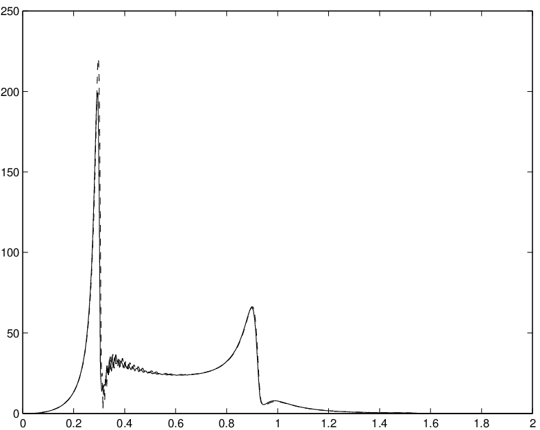
An example of these results is given in fig. 7.2.

7.3 The cumulative contributions of the SBW1, SBW2 and SSW to the overall frequency domain ground response

The discussion here centers on the transfer functions of frequency domain ground response. In all that follows, the graph of the modulus of $I_{1}^{1}(\mathbf{x}_{g},\nu)/u^{i}(\mathbf{x}_{g},\nu)$ versus frequency $\nu$ is designated by dots, the graph of the modulus of $I_{2}^{1}(\mathbf{x}_{g},\nu)/u^{i}(\mathbf{x}_{g},\nu)$ versus $\nu$ is designated by dashes, the graph of the modulus of $(I_{2}(\mathbf{x}_{g},\nu)^{1}+I_{3}^{1}(\mathbf{x}_{g},\nu))/u^{i}(\mathbf{x}_{g},\nu)$ versus frequency $\nu$ is designated by dot-dashes, and the graph of the modulus of the ground displacement $u(\mathbf{x}_{g},\nu)/u^{i}(\mathbf{x}_{g},\nu)$ versus frequency by a continuous line.

To begin, consider a configuration thought to be representative of that in the central portion of the city of Nice (France) wherein $c^{0}=1000$ m/s, $\rho^{1}=1800$ kg/m³, $c^{1}=200$ m/s.

We first place the source at a relatively-large depth of 3km on the $x_{2}$ axis, i.e., $\mathbf{x}^{s}=(0\text{m},3000\text{m})$ and evaluate the moduli of the ground transfer functions relatively near the epicenter, i.e., $\mathbf{x}=(100\text{m},0\text{m})$ (left subfigure in fig. 7.3) as well as relatively far from the epicenter, i.e., $\mathbf{x}=(3000\text{m},0\text{m})$ (middle subfigure in fig. 7.3), and then place the source at a relatively-small depth of 100m on the $x_{2}$ axis, i.e., $\mathbf{x}^{s}=(0\text{m},100\text{m})$ and evaluate the ground transfer functions relatively far from the epicenter, i.e., $\mathbf{x}=(3000\text{m},0\text{m})$ (right subfigure in fig. 7.3).

It will be noticed that, in this and practically all subsequent results, the curve relative to $\big|(I_{2}^{1}(\mathbf{x}_{g},\nu)+I_{3}^{1}(\mathbf{x}_{g},\nu))/u^{i}(\mathbf{x}_{g},\nu)\big|$ is coincident with that relative to $\big|I_{2}^{1}(\mathbf{x}_{g},\nu)/u^{i}(\mathbf{x}_{g},\nu)\big|$ which means, as predicted by the analysis of the preceding section, that the contribution to overall ground response of the standing surface waves in the layer is negligible. Thus, we restrict the following discussion to the sole contribution of the standing bulk waves of the first (SBW1) and second kinds (SBW2). The left and middle panels in fig. 7.3 show that when the the focal depth is large the ground response is largely dominated by the contribution of the SBW1 (i.e., by $|I_{1}^{1}(\mathbf{x}_{g},\nu)/u^{i}(\mathbf{x}_{g},\nu)|$ ), and, in fact, the SBW2 have no influence on the response beyond $\sim 1$ Hz. However, the right panel in fig. 7.3 gives just the opposite result when the focal depth is small, since the ground response is largely dominated by the SBW2 (i.e., by $|I_{2}^{1}/S(\omega)|$ ) and the SBW1 have little influence beyond $\sim 1$ Hz. Another interesting feature of these results is that the total response curves have noticeably-different appearance when the source is deep or shallow (notice that this appearance is qualitatively the same for small and large epicentral distances, assuming the same, large focal depths in the two cases).

Next consider a somewhat softer environment than in Nice

wherein $c^{0}=600$ m/s, $\rho^{1}=1300$ kg/m³, $c^{1}=200$ m/s (fig. 7.4). We first place the source (rather deep) at $\mathbf{x}^{s}=(0\text{m},3000\text{m})$ and evaluate the ground transfer functions relatively far from the epicenter, i.e., $\mathbf{x}=(3000\text{m},0\text{m})$ (left subfigure in fig. 7.4), and then place the source at a relatively-small depth, i.e., $\mathbf{x}^{s}=(0\text{m},100\text{m})$ , and again evaluate the ground transfer functions relatively far from the epicenter, i.e., $\mathbf{x}=(3000\text{m},0\text{m})$ (right subfigure in fig. 7.4). We again observe that the ground response is dominated by the SBW1 when the source is deep and by the SBW2 when the source is shallow. Also we notice that the appearance of the total response curve for a deep source is different from than of a shallow source.

We next consider a Mexico-city like site (of course without the buildings, contrary to the case in [12])

in which $c^{0}=600$ m/s, $\rho^{1}=1300$ kg/m³, $c^{1}=60$ m/s (fig. 7.5). In all except the lower right hand panel we again observe that the ground response is dominated by the SBW1 when the source is deep and by the SBW2 when the source is shallow. The exceptional case is that of a shallow source and small epicentral distance, for which the contributions of the SBW2 and SBW1 to the overall response are of comparable magnitude, especially near the first low frequency peak. A plausible cause of this behavior is the rather large contrast of body-wave velocities between the the layer and substratum, thus giving rise to a large contribution of the individual SBW1 at the fundamental Haskell frequency (recall that this contribution is all the greater the greater the body wave velocity contrast).

Next we consider a Mexico City-like environment with a somewhat harder substratum for which $c^{0}=1500$ m/s, $\rho^{1}=1300$ kg/m³, $c^{1}=60$ m/s (fig. 7.6). For a deep source and large epicentral distance (left panel of the figure), the response is dominated, as usual, by the SBW1. When the source is shallow and the epicentral distance is large (right panel of the figure) we encounter a new kind of response characterized by contributions of the SBW1 and SBW2 that are of comparable magnitude (this was obtained in the previous figure for a shallow source and small epicentral distance. That this should occur even for a large epicentral distance is probably attributable to the fact that the body wave velocity contrast is very large (it was smaller in the configuration of the previous figure) which fact favorizes a substantial contribution of the SBW1 (notably near the fundamental Haskell frequency), even when the distance between the source and observation point is large.

The last result in this series concerns once again the Mexico City-like environment in which $c^{0}=600$ m/s, $\rho^{1}=1300$ kg/m³, $c^{1}=60$ m/s (fig. 7.7). We are now interested in evaluating the effect of changes in the layer thickness $h$ for a shallow source and large epicentral distance. We observe in the figure that the response is dominated by the cumulative contribution of the SBW2 for all the layer thicknesses. Furthermore, the number and finesse of the resonance peaks in the interval $[0,2{\text{H}z}]$ increases with $h$ , the dominant peak always being the one associated with the resonant excitation of the first (lowest-frequency) Love mode and being located at a frequency that is all the lower the larger is $h$ .

7.4 Time records of various input pulses for different combinations of source and observation point coordinates

In the following, we exhibit (figs. 7.8-7.10) time records of the three pseudo-Ricker pulses having frequencies: $\nu_{0}=0.25$ Hz, 0.5Hz, 1.0Hz (whose spectra were shown previously in fig. 7.1). This is done for all combinations of the four coordinates (assuming $x_{1}^{s}=0$ m, $x_{2}=0$ m): $x_{2}^{s}=100$ m, $x_{2}^{s}=3000$ m, $x_{1}=100$ m, $x_{1}=3000$ m.

As expected, the pulses have the same shape for all source and observation point locations since the substratum was assumed to be an elastic (i.e., non-dispersive) medium; however their maxima change as a function of these locations. Not unexpectedly, the largest pulses are those for which the source to observation point distances are the smallest. Of particular interest is the fact that the input pulse duration is approximately $2/\nu_{0}$ , which corresponds to $\sim$ 8s for the 0.25Hz pulse, $\sim$ 4s for the 0.5Hz pulse, and $\sim$ 2s for the 1.0Hz pulse. As will be seen hereafter, the response to these pulses in the layered configuration is generally of much longer duration.

7.5 Comparison of frequency and time domain responses for constant source-to-observation point distances

Again, we begin by a configuration thought to be representative of that in the central portion of the city of Nice (France) wherein $c^{0}=1000$ m/s, $\rho^{1}=1800$ kg/m³, $c^{1}=200$ m/s. Two constant source-to-observation point distance situations are considered: a) $\mathbf{x}^{s}=(0\text{m},3000\text{m})$ , $\mathbf{x}=(100\text{m},0\text{m})$ (solid line curves in fig. 7.11), and b) $\mathbf{x}^{s}=(0\text{m},100\text{m})$ , $\mathbf{x}=(3000\text{m},0\text{m})$ (dotted line curves in fig. 7.11).

We notice in the left panel of fig. 7.11 that the first bump of the transfer function occurs at a lower frequency when the source is near to the layer than when it is far from the layer, which fact suggests that the lower-frequency bump is due to the (resonant) excitation of the fundamental Love mode (SBW2) whereas the higher-frequency peak is associated with the first (non-resonant) interference (SBW1) maximum. The same remarks apply to the higher-order bumps. Moreover, the value of the transfer function at the first couple of bumps is much larger due to Love mode excitation than to constructive interference effects, and since the widths of these two bumps are approximately the same, the finesse (height/width ratio) of the Love mode peak is larger than that of the interference peak. The translation of this into the time domain is that the signal associated mainly with the fundamental Love mode resonance is more intense and of longer duration than the signal associated mainly with the fundamental interference bump.

This last remark should be tempered by consideration of the spectrum of the input pulse, since the transfer functions do not take this spectrum into account whereas the temporal signals do. Thus, when the location of the maximum of the spectrum of the input pulse is closer to the location of the maximum of the transfer function, the time-domain response is larger, as seen in fig. 7.12, this being true for signals that are essentially due both to Love resonances or to constructive interference effects (note that the location of the pulse maxima were adjusted so as to be close to the locations of the transfer function fundamental peaks). Actually, this figure reveals the existence of a beating phenomenon in the ground response temporal signal for a source near the layer, which is probably due to the combined (amplitude modulation) effects of the fundamental Love mode peak and the fundamental interference peak. This issue will be discussed in more depth in the next section.

Next consider the somewhat softer-than-in-Nice environment

wherein $c^{0}=600$ m/s, $\rho^{1}=1300$ kg/m³, $c^{1}=200$ m/s (fig. 7.13). Again, the two source/observation point couples are: $\mathbf{x}^{s}=(0\text{m},3000\text{m})$ , $\mathbf{x}=(3000\text{m},0\text{m})$ (solid line curve in fig. 7.13 and $\mathbf{x}^{s}=(0\text{m},100\text{m})$ , $\mathbf{x}=(3000\text{m},0\text{m})$ (dotted line curve in fig. 7.13). All that was said in the previous example concerning the transfer functions holds in the present case. Likewise, the repercussions on the temporal signals are the same as in the previous case (short duration signal for a remote source and relatively-long signal for a near source.

We next consider a Mexico-city like site (again, without the buildings)

in which $c^{0}=600$ m/s, $\rho^{1}=1300$ kg/m³, $c^{1}=60$ m/s (fig. 7.14). Again, the two source/observation point couples are: $\mathbf{x}^{s}=(0\text{m},3000\text{m})$ , $\mathbf{x}=(3000\text{m},0\text{m})$ (solid line curve in fig. 7.14) and $\mathbf{x}^{s}=(0\text{m},100\text{m})$ , $\mathbf{x}=(3000\text{m},0\text{m})$ (dotted line curve in fig. 7.14). All that was said in the two previous examples concerning the transfer functions holds in the present case. Likewise, the repercussions on the temporal signals are the same as in the previous two cases (short duration signal for a remote source and relatively-long signal for a near source.

7.6 Time domain responses for very large and very small source-to-observation point distances

We again consider a Mexico-city like site

at which $c^{0}=600$ m/s, $\rho^{1}=1300$ kg/m³, $c^{1}=60$ m/s (fig. 7.15). Although in fig. 7.5 upper left and lower right panels) we observed that the transfer functions for very large and very small source-to-observation point distances are qualitatively very similar, we are somewhat surprized to find that the two corresponding signals in fig. 7.15 are so qualitatively similar, due to the fact that the transfer function corresponding to the left panel in fig. 7.5 is dominated by the SBW1 contribution, whereas the transfer function corresponding to the right hand panel in fig. 7.5 has strong contributions from both the SBW1 and SBW2. The clue to this unexpected result resides in the spectrum of the $\nu_{0}=0.5$ Hz input pulse (see middle panel of fig. 7.1), since the maximum of the latter is around $\nu_{0}=0.6$ Hz and this frequency is both far-removed form the peaks of the transfer functions and characterized by a predominant contribution of the SBW1 (the latter fact providing an explanantion of the relatively-short duration of the response signals in fig. 7.15 (note that the intensity of the very close source-to-observation point signal is much larger than that of the other signal, as it should be).

7.7 Time domain responses for different input pulses and fixed source and observation point coordinates

It is of considerable interest to ascertain to what extent the spectrum of the source affects the ground response [18], notably when the source is near the layer.

In fig. 7.16 (which again applies to the Mexico City like environment), we see, as expected, that when the spectrum of the input pulse is such as to overlap substantially the frequency band covered by the fundamental Love mode peak (left and middle panels in fig. 7.16), the duration of the signal is large. When the spectrum of the input pulse is such as to overlap substantially the frequency band covered by the second Love mode peak (right panel in fig. 7.16), the duration of the signal is smaller than in the previous case due to the smaller finesse of the second Love mode resonance peak. In all three cases, we observe some beating, presumably due to the proximity of the interference peak and Love resonance peak in the transfer function.

7.8 Time domain responses for various layer thicknesses and input pulses

A more thorough study of the influence of the input spectrum must take into account variations of the layer thickness.

This is done (again in the Mexico City-like environment and for a source that is 100m below the ground) in fig. 7.17 for a 20m thick layer, in fig. 7.18 for a 40m thick layer, in fig. 7.19 for a 60m thick layer, and in fig. 7.20 for a 90m thick layer. We observe quite different responses, varying from a short pulse quite similar to the input pulse (for the thinnest layer and the lowest frequency input pulse) to a very long duration pulse (as much as 200s as compared to the the 4s duration of the input pulse) with pronounced beating (for the thickest layer and a medium frequency input pulse). Note that the 90m layer also corresponds to the case in which the source is closest to the layer (10m from the bottom face of the layer), which may also be a factor contributing to the pronounced anomalous character of the response in this configuration.

Finally, we consider a Mexico City-like environment with a somewhat harder substratum for which $c^{0}=1500$ m/s, $\rho^{1}=1300$ kg/m³, $c^{1}=60$ m/s (fig. 7.21). Two constant source-to-observation point distance situations are again considered: a) $\mathbf{x}^{s}=(0\text{m},3000\text{m})$ , $\mathbf{x}=(100\text{m},0\text{m})$ (solid line curves in fig. 7.21), and b) $\mathbf{x}^{s}=(0\text{m},100\text{m})$ , $\mathbf{x}=(3000\text{m},0\text{m})$ (dotted line curves in fig. 7.21). For a deep source and large epicentral distance, the frequency response (in the left hand panel of the figure) is dominated, as usual, by the fundamental interference peak, and this results in a relatively-long duration time domain signal (solid line curve in the right hand panel of the figure) in response to a $\nu_{0}=0.5$ Hz input pulse. When the source is shallow and the epicentral distance is large the frequency response is dominated, unsurprizingly, by the fundamental Love mode resonance peak, and this gives rise to a somewhat longer-duration signal (dotted line curve in the right hand panel of the figure) in response to the $\nu_{0}=0.5$ Hz input pulse. This example indicates that it may be difficult to distinguish between the contributions of the SBW1 and SBW2 when the contrast of the material properties between the layer and the substratum is very large.

7.9 Regional path effects

We now examine the manner in which a wave radiated from a source located underneath, but close to, the lower crustal boundary propagates over long distances.

An example (real) of such motion, relative to the 11-3-02 (shallow) seismic Denali (Alaska) event recorded at a free-field ground location (i.e., 1.5km from the buildings of the city of Anchorage) at an epicentral distance of more than 275km is given in fig. 10 of [6]. A remarkable feature of this motion is its long duration of over 125s. We will show that this is possible with our simple model.

We constructed a hopefully-plausible crustal model starting with the parameters of a thin layer, softer-than-Nice like configuration (for which $\rho_{0}=2000$ kg/m³, $\rho_{1}=1300$ kg/m³, $c^{0}=600$ m/s, $c^{1}=200$ m/s, $Q^{0}=\infty$ , $Q^{1}=30$ , $h=80$ m), and by assuming conservation of such quantities as $k^{1}h$ , $\rho^{0}/\rho^{1}$ , etc. in going to a much thicker layer. Let us suppose that we have two configurations, one of which is thin-layered and known (configuration with subscript 1), and the other is thick-layered and unknown (configuration with subscript 2). The layer in the known configuration is relatively soft and lossy, whereas it is relatively hard (although always softer than the substratum) in the unknown configuration. Since harder media are usually less lossy, we assume rather arbitrarily that the $Q$ of the layer in the unknown configuration is 20 times larger than the $Q$ in the known configuration, while the $Q$ ’s of the substratum remain infinite in both configurations. Thus, we have: $Q^{0}_{2}=Q^{0}_{1}=\infty$ and $Q^{1}_{2}=20Q^{1}_{1}=600$ . Conservation of $k^{1}h$ means $k^{1}_{1}h_{1}=k^{1}_{2}h_{2}$ , whence $c^{1}_{2}=c^{1}_{1}\nu_{2}h_{2}/\nu_{1}h_{1}$ , or, if we choose $\nu_{1}=1$ Hz, $\nu_{2}=0.08$ Hz, and $h_{2}=10km$ , then $c_{2}=2000$ m/s. Conservation of $\rho^{0}/\rho^{1}$ means $\rho^{0}_{1}/\rho^{1}_{1}=\rho^{0}_{2}/\rho^{1}_{2}$ , so that if we choose $\rho^{0}_{2}=2600$ kg/m³ (close to the density of granite), then $\rho^{1}_{2}=1690$ kg/m³. We would also like to conserve wavespeed proportions, i.e., $c^{0}_{1}/c^{1}_{1}=c^{0}_{2}/c^{1}_{2}$ , but this turns out to give wavespeeds in $M^{0}$ that are much larger than those for granite (3200m/s) for the choice $c^{1}_{2}=2000$ m/s, so that we arbitrarily chose $c^{0}_{2}=3000$ m/s (i.e., close to the wavespeed in granite). Finally we chose to conserve the relative distance of the source to the lower boundary of the layer, i.e., $(x_{2}^{s}-h)/x_{2}^{s}$ , which gives $x_{2}^{s}=12$ km.

The results for this new (crustal) configuration excited by the usual pseudo-Ricker pulse line sources are given in fig. 7.22 wherein it can be seen that the ground response far from the epicenter (300km): 1) is dominated by the excitation of Love modes (notably the fundamental), 2) takes the form of a pulse which has a shape not very different from that in fig. 10 of [6] and is of approximately 100s duration, governed essentially by the fundamental Love resonance peak. Thus, our theoretical model shows that it is quite possible for a source underneath, and relatively close to, a fairly thick, fairly hard crust overlying a very hard substratum to give rise to a rather long-duration pulse even at large epicentral distances. What becomes of this pulse when a city is located at this large lateral distance from the source constitutes an important, and as yet not fully-elucidated, question (this meaning, that although studies such as [9] are designed to take into account all that occurs between the distant source and the observation point in the basin, the results that are offered are entirely of numerical nature and therefore do not provide an explanation of the underlying physical processes).

8 Phenomenological model of the time-domain
ground response

In sect. 6 we mentioned the difficulties of obtaining closed-form expressions of the integrals $I_{1}^{1}$ , $I_{2}^{1}$ and $I_{3}^{1}$ and therefore of the Fourier integral (3.35) accounting for the time-domain ground response. Nevertheless, the many numerical examples in sect. 7 of the frequency-domain ground response all seem to have common features which we shall attempt to describe in this section in phenomenological manner. Moreover, this approach will be shown to provide a simple means of understanding the origin of the main features of the time domain response.

The principal features of the ground transfer function $|u(\mathbf{x}_{g},\omega)/u^{i}(\mathbf{x}_{g},\omega)|$ appeared to be due to interference and resonance causes and manifested themselves by a series of well-defined, regularly-spaced bumps. That the nature of these bumps be due either to interference or to resonance causes is not of primal importance at the present (phenomenological) level of analysis; the only aspects that interest us now are the relative widths and heights of the bumps (recall that, in general, the bumps associated with interferences (SBW1) are broader and less intense than the corresponding bumps associated with Love mode resonances (SBW2)).

We represent each of these bumps by a gaussian function of frequency, which we multiply by the spectrum $S(\omega)$ of the incident pulse and by an amplitude function $\mathcal{A}(\mathbf{x}_{g},\mathbf{x}^{s},\omega)$ of $\mathbf{x}_{g}$ , $\mathbf{x}^{s}$ and $\omega$ to take into account the fact (observed in the numerical results) that the different bumps of frequency-domain response indeed depend on these quantitites. Let $G_{l}(\omega)$ be the $l$ -th gaussian function of the form

G_{l}(\omega)=\frac{1}{\sqrt{\pi\varepsilon_{l}}}e^{-\frac{(\omega-\omega_{l})^{2}}{\varepsilon_{l}}}~.

(8.1)

The bump connected with this function attains its maximum at $\omega=\omega_{l}$ and its finesse is all the larger, the smaller is $\varepsilon_{l}$ . In fact [56] (p. 319), $G_{l}(\omega)$ tends towards the Dirac delta distribution $\delta(\omega-\omega_{l})$ as $\varepsilon_{l}\rightarrow 0$ .

Thus, we represent the frequency-domain ground response by

u^{1}(\mathbf{x}_{g},\omega)\approx\sum_{l=1}^{L}S(\omega)\mathcal{A}_{l}(\mathbf{x}_{g},\mathbf{x}^{s},\omega)G_{l}(\omega)~,

(8.2)

wherein $\omega_{l+1}>\omega_{l}$ and $L$ may be a large positive integer. However, the latter will be taken equal to 4 due to the fact that we assume that the spectrum $S(\omega)$ of the input pulse is not too broad and centered at low frequencies (the case of interest in the applications considered herein). Introducing (8.2) into (3.35) gives

u^{1}(\mathbf{x}_{g},t)\approx 2\Re\sum_{l=1}^{4}\int_{0}^{\infty}S(\omega)\mathcal{A}_{l}(\mathbf{x}_{g},\mathbf{x}^{s},\omega)G_{l}(\omega)e^{-i\omega t}d\omega~.

(8.3)

Although we don’t know, nor assume, much about $S$ and $\mathcal{A}_{l}$ , it seems reasonable to suppose that these functions are slowly-varying in comparison to $G_{l}(\omega)$ with respect to $\omega$ in the neighborhoods $\omega_{l}$ in which the gaussians are maximal. Consequently, we can make the approximation

u^{1}(\mathbf{x}_{g},t)\approx 2\Re\sum_{l=1}^{4}S(\omega_{l})\mathcal{A}_{l}(\mathbf{x}_{g},\mathbf{x}^{s},\omega_{l})\int_{0}^{\infty}G_{l}(\omega)e^{-i\omega t}d\omega~.

(8.4)

By proceeding as in [56] (p.313) and making use of the identity [52] $\int_{0}^{\infty}\exp(-\xi^{2})d\xi=\sqrt{\pi}/2$ , we find

\int_{0}^{\infty}G_{l}(\omega)e^{-i\omega t}d\omega=e^{-\frac{\varepsilon_{l}}{4}t^{2}-i\omega_{l}t}~,

(8.5)

so that

u^{1}(\mathbf{x}_{g},t)\approx 2\Re\sum_{l=1}^{4}S(\omega_{l})\mathcal{A}_{l}(\mathbf{x}_{g},\mathbf{x}^{s},\omega_{l})e^{-\frac{\varepsilon_{l}}{4}t^{2}-i\omega_{l}t}~.

(8.6)

By representing $S$ and $\mathcal{A}_{l}$ in polar form

S(\omega_{l})=|S(\omega_{l})|e^{i\sigma_{l}(\omega_{l})}~~~,~~~\mathcal{A}_{l}(\mathbf{x}_{g},\mathbf{x}^{s},\omega_{l})=|\mathcal{A}_{l}(\mathbf{x}_{g},\mathbf{x}^{s},\omega_{l})|e^{i\alpha_{l}(\mathbf{x}_{g},\mathbf{x}^{s},\omega_{l})}~,

(8.7)

we get

u^{1}(\mathbf{x}_{g},t)\approx\Re\sum_{l=1}^{4}\mathcal{B}_{l}(\mathbf{x}_{g},\mathbf{x}^{s},\omega_{l})e^{-\frac{\varepsilon_{l}}{4}t^{2}-i\left[\omega_{l}t-\beta_{l}(\mathbf{x}_{g},\mathbf{x}^{s},\omega_{l})\right]}=\\ \sum_{l=1}^{4}\mathcal{B}_{l}(\mathbf{x}_{g},\mathbf{x}^{s},\omega_{l})e^{-\frac{\varepsilon_{l}}{4}t^{2}}\cos\left(\omega_{l}t-\beta_{l}(\mathbf{x}_{g},\mathbf{x}{s},\omega_{l})\right)~,

(8.8)

wherein

\mathcal{B}(\mathbf{x}_{g},,\mathbf{x}^{s},\omega_{l}):=2|S(\omega_{l})||\mathcal{A}_{l}(\mathbf{x}_{g},\mathbf{x}^{s},\omega_{l})|,\\ \beta_{l}(\mathbf{x}_{g},\mathbf{x}^{s},\omega_{l}):=\alpha_{l}(\mathbf{x}_{g},\mathbf{x}^{s},\omega_{l})+\sigma(\omega_{l})~.

(8.9)

With this in hand, we now try to account for the main features of the numerical results pertaining to the time records of ground response.

Assume that one of the bumps in the ground transfer function dominates all others. In the present paradigm, this signifies that one of the terms, say the $m$ -th in the sum in (8.8) dominates all the others. As observed in the numerical results, this term should account either for the fundamental Love mode resonance ( $m$ =1) or for the fundamental interference peak ( $m$ =2), the necessary condition for the Love peak to be dominant being that the source is close to the bottom boundary of the layer, and the necessary condition for the interference peak to be dominant being that the source is far from the bottom boundary of the layer. In either case, we have:

u^{1}(\mathbf{x}_{g},t)\approx\mathcal{B}_{m}(\mathbf{x}_{g},\mathbf{x}^{s},\omega_{m})e^{-\frac{\varepsilon_{m}}{4}t^{2}}\cos\left(\omega_{m}t-\beta_{m}(\mathbf{x}_{g},\mathbf{x}^{s},\omega_{m})\right)~,

(8.10)

which is indicative of the existence of a monochromatic wave (angular frequency $\omega_{m}$ ) whose amplitude $\mathcal{B}_{m}$ and phase $\beta_{m}$ vary with the positions of the source and the observation point on the ground, and which is exponentially-attenuated with time. This attenuation is more or less pronounced, so that the duration of the signal is large if $\varepsilon_{m}$ is small (i.e., the finesse of the corresponding transfer function bump is large) as would occur for a Love mode resonance, and is relatively small if $\varepsilon_{m}$ is relatively large (i.e., the finesse of the corresponding transfer function bump is relatively small) as would generally occur for an interference peak. The same phenomenon is produced, although with less intensity due to the lowering of $|\mathcal{B}_{m}|$ , if the spectrum of the incident pulse is such as to favorize either the second Love mode resonance or the second interference peak rather than the fundamental Love mode resonance or the fundamental interference peak.

Consider a different type of situation in which two bumps in the ground transfer function dominate all others. In the present paradigm this means that two terms in (8.8), say the $m$ -th and $n$ -th, dominate all the others, i.e.,

u^{1}(\mathbf{x}_{g},t)\approx\mathcal{B}_{m}(\mathbf{x}_{g},\mathbf{x}^{s},\omega_{m})e^{-\frac{\varepsilon_{m}}{4}t^{2}}\cos\left(\omega_{m}t-\beta_{m}(\mathbf{x}_{g},\mathbf{x}^{s},\omega_{m})\right)+\\ \mathcal{B}_{n}(\mathbf{x}_{g},\mathbf{x}^{s},\omega_{n})e^{-\frac{\varepsilon_{n}}{4}t^{2}}\cos\left(\omega_{n}t-\beta_{n}(\mathbf{x}_{g},\mathbf{x}^{s},\omega_{n})\right)~.

(8.11)

The numerical results in the previous section show that this occurs only when the $m$ -th term corresponds to a Love mode resonance and the $n$ -th term to the interference peak nearest the Love mode resonance peak, so that $n=m+1$ in the present numbering system. Moreover, the most pronounced phenomena were shown numerically to be produced when the fundamental Love mode resonance and fundamental interference peak are involved, so that $m=1$ , $n=2$ is the most interesting case.

We can write (e.g., for $m=1$ , $n=2$ )

u^{1}(\mathbf{x}_{g},t)\approx\mathcal{B}_{1}e^{-\frac{\varepsilon_{1}}{4}t^{2}}\mathcal{C}_{1}+\mathcal{B}_{2}e^{-\frac{\varepsilon_{2}}{4}t^{2}}\mathcal{C}_{2}=\\ \left(\mathcal{B}_{1}e^{-\frac{\varepsilon_{1}}{4}t^{2}}+\mathcal{B}_{2}e^{-\frac{\varepsilon_{2}}{4}t^{2}}\right)\frac{\mathcal{C}_{1}+\mathcal{C}_{2}}{2}+\left(\mathcal{B}_{1}e^{-\frac{\varepsilon_{1}}{4}t^{2}}-\mathcal{B}_{2}e^{-\frac{\varepsilon_{2}}{4}t^{2}}\right)\frac{\mathcal{C}_{1}-\mathcal{C}_{2}}{2}~,

(8.12)

so that

u^{1}(\mathbf{x}_{g},t)\approx\left(\mathcal{B}_{1}e^{-\frac{\varepsilon_{1}}{4}t^{2}}+\mathcal{B}_{2}e^{-\frac{\varepsilon_{2}}{4}t^{2}}\right)\times\\ \cos\left[\frac{(\omega_{1}+\omega_{2})t}{2}-\frac{\beta_{1}+\beta_{2}}{2}\right]\cos\left[\frac{(\omega_{1}-\omega_{2})t}{2}-\frac{\beta_{1}-\beta_{2}}{2}\right]-\\ \left(\mathcal{B}_{1}e^{-\frac{\varepsilon_{1}}{4}t^{2}}-\mathcal{B}_{2}e^{-\frac{\varepsilon_{2}}{4}t^{2}}\right)\times\\ \sin\left[\frac{(\omega_{1}+\omega_{2})t}{2}-\frac{\beta_{1}+\beta_{2}}{2}\right]\sin\left[\frac{(\omega_{1}-\omega_{2})t}{2}-\frac{\beta_{1}-\beta_{2}}{2}\right]~.

(8.13)

An interesting case is: $\mathcal{B}_{1}\approx\mathcal{B}_{2}$ , $\varepsilon_{1}\approx\varepsilon_{2}$ , whence

u^{1}(\mathbf{x}_{g},t)\approx\\ 2\mathcal{B}_{1}e^{-\frac{\varepsilon_{1}}{4}t^{2}}\cos\left[\frac{(\omega_{1}+\omega_{2})t}{2}-\frac{\beta_{1}+\beta_{2}}{2}\right]\cos\left[\frac{(\omega_{1}-\omega_{2})t}{2}-\frac{\beta_{1}-\beta_{2}}{2}\right]~,

(8.14)

which is indicative of monochromatic sinusoidal motion of angular frequency $\frac{\omega_{1}+\omega_{2}}{2}$ , amplitude-modulated by an attenuated sinusoid of frequency $|\frac{\omega_{1}-\omega_{2}}{2}|$ . In this case, the signal associated with the ground motion exhibits the beating and attenuation observed in some of the computed results, with the duration depending, as in the previous case, on the finesse of the resonance and interference bumps.

Actually, it is not necessary for $\mathcal{B}_{1}\approx\mathcal{B}_{2}$ , $\varepsilon_{1}\approx\varepsilon_{2}$ in order to have beating in the signal, since although the motion associated with (8.13) is more complicated than that of (8.14), in both cases a form of attenuated signal with more or less regular beating is present. The signal with irregular beating predicted by (8.14) is the case most commonly observed in the computed results of the previous section.

Thus, the phenomenological model accounts for all of the features of the computed time records: quasi-monochromatic attenuated signals (whose duration is governed by the finesse of the frequency domain bump) without beating when either the Love mode resonance or interference peak is involved, an attenuated signal with regular beating when the frequency domain bumps are of comparable magnitude and finesse (the latter governing the duration of the signal), an attenuated signal with irregular beating when the magnitude and finesse of the fundamental Love and interference bumps are rather different.

9 Discussion

We shall now attempt to provide answers to the questions raised in sect. 1.

The first question was: is it possible to obtain anomalous response without any lateral heterogeneity in the underground medium? The configuration studied herein was laterally- homogeneous. We have shown that 1D response only accounts for interference effects (as embodied by the SBW1), but not for coupling to Love modes (as embodied by the SBW2) in the layer, which is particularly strong when the source is in the neighborhood of the lower boundary of the layer. Insofar as anomalous effects are essentially characterized by long duration and beating phenomena in the signals (e.g., curves in the middle and right panels of fig. 7.19), the answer to this question is negative as concerns 1D response. However, when the contrast of material properties between the layer and substratum is very large, it is possible to obtain fairly-long duration signals (albeit without beating), which are essentially associated with 1D response, even when the source is far from the lower boundary of the layer (solid curve in right panel of fig. 7.21). More generally, i.e., when coupling to Love modes is achieved, the answer to the question is positive.

The second question was: what is the relation of 1D to 2D response and how adequate is it to model the general response of the configuration by its response to a (nearly) vertically-incident plane wave? We have shown that not only does the 1D model not give rise to resonance phenomena, but that truly-resonant phenomena associated with the excitation of Love modes can only be described by a fully 2D (or 3D) model. For a source far from the lower boundary of the layer, the response is essentially due to the contributions of the SBW1 (more or less equivalent to the 1D response), but when the source is near this boundary, the waves (SBW2) not included in the 1D model play a major role in the overall response in that they either overwhelm the 1D response (long duration response without beating) or combine with the 1D response to produce signals with long duration and beating. This finding should be taken into account in relation to studies (e.g., [14]) that attempt to predict seismic response of urban sites from 1D type of analysis.

The third question was: how does the focal distance of the source affect the response? The answer to this question was already provided in the previous two paragraphs. However, it is opportune to reconsider this question in the light of topic (b) concerning the effects of underlying soil heterogeneities, lateral variations of the underlying soil layer, and built environment on seismic response in urban sites. One can show ([57]) that a wave incident on a heterogeneous medium gives rise to a diffracted wave which can be considered to be radiated by induced sources (as opposed to the active source associated with the primary seismic disturbance) located within the medium. These induced sources can also appear on the boundary of the medium (especially at endpoints, corners and irregularities of the boundary), so that the edges of a soft basin or the stress-free ground which includes the buildings overlying a homogeneous soft layer in a city-like site, can also constitute the locations of intense induced sources in response to an incident seismic wave. The fields radiated by all these induced sources can be represented in a manner identical (provided the basic geometry of the configuration is similar) to that of the present work, so that much of what was written and found above, notably concerning the response to active sources located outside, and in the vicinity of the soft layer (and, by extension, to induced sources located within or on the boundaries of the soft layer, should apply to city-like sites built on soft layers or basins. The most important point (mentioned in references such as [12], implicit in [20], [21], and proven herein as concerns active sources) is the following: the presence of these active or induced sources, located near or within the soft layer overlying a relatively-hard substratum, enables coupling to Love-type modes which are responsible for a part of the anomalous ground response observed in cities such as Mexico, notably motion characterized by long durations and beatings.

The fourth question was: how does the epicentral distance affect the response? We have shown that the epicentral distance ( $|x_{1}-x_{1}^{s}|$ , for $\mathbf{x}_{g}=(x_{1},0$ ) is not as sensitive as other parameters (especially the focal distance $|0-y_{1}^{s}|$ ) as concerns its influence on duration and on the presence or absence of beatings in the ground motion (it should be mentioned that in [58] the duration appears to be a linearly-increasing function of epicentral distance, but the slope of this function decreases when the crustal layer is softer). However, the epicentral distance (more generally: the distance of the source to the observation point) is a critical factor in determining the intensity of the signal on the ground (see, e.g., figs. 7.14-7.15).

The fifth question was: how does the contrast of mechanical properties between the layer and the half space affect the ground response? There does not appear to exist a clear-cut answer to this question (see, however, [58] in which it appears rather systematically that softer layers lead to longer durations and lower peak response for a given epicentral distance), since the dependence on the mechanical parameters is very much intermingled with that on the values of the geometrical and source parameters. On the whole, most of the answers to the previous four questions hold in a qualitative sense whatever the contrast of mechanical properties (see, e.g., the results herein for Nice, softer Nice, Mexico, Mexico with harder substratum), although there are some quantitative differences (e.g., the contrast influences considerably the intensity of the SBW1 contribution). Naturally, the most remarkable features of the ground response of our simple configuration, which are due to the excitation of the fundamental Love mode, can only be observed if the layer is softer than the substratum in the sense of (5.3) and (5.4). These conditions are so broad and widespread (for city-like sites) as to render the ’anomalous’ response described herein a quite universal phenomenon.

The sixth question was: how does the thickness of the layer affect the response? In fig. 7.7 it was found that increasing the layer thickness increases the number of peaks, as well as the finesse of each of the latter, in a given range of frequencies of the transfer function. This has the effect of lowering the frequency of occurrence of the first peak so that the time-domain response will be largely conditioned by the spectrum of the input pulse, assuming the latter to be centered at a relatively high frequency. Thus, a low frequency pulse can produce substantially the same type of response for a thick layer as a relatively high frequency pulse in a thin layer. This point is important in connection with the topic of regional path effects mentioned in sect. 1.

The seventh question was: how do the spectral characteristics of the incident pulse affect the response? The answer to this question can be found by comparing the three subfigures in any one of figs. 7.17-7.20. Obviously, the spectrum of the incident pulse is a key factor (see sect. 8), which: a) if it overlaps either a constructive interference peak or Love mode peak, gives rise to attenuated, quasi monochromatic response, often of long duration (see figs. 7.17-7.20 in which an example is given of a pulse having a duration of 4s that gives rise to substantial ground response of 200s duration), b) if it overlaps both a constructive interference peak and Love mode peak, gives rise to attenuated, quasi monochromatic response with more or less regular beatings, c) if it doesn’t overlap significantly either a constructive interference of Love mode peak, gives rise to a time domain response that can be qualitatively quite similar to the input signal (see, e.g., left panel of fig. 7.18). When the sources are induced, their spectra will be modified with respect to that of the spectrum of the primary active source due to diffraction and dispersion, so that an a priori unfavorable situation for anomalous response from the point of view of the primary active source may turn out to be favorable from the point of view of the induced sources.

10 Conclusion and perspectives

This work originated in the observation that no satisfactory physical explanation has been given until now of anomalous seismic response in urban environments with soft layers or basins overlying a hard substratum. The principal reason for this knowledge gap probably lies in the complexity of the sites examined in previous (essentially-numerical) studies: 1) a homogeneous or multilayered basin of complicated form not including buildings (e.g., [13], [9], [59]), 2) a homogeneous layer overlain by a periodic or non-periodic set of blocks or buildings (e.g., [12], [31]). The choice was therefore made herein to simplify as much as possible the characteristics of the site and sollicitation, while retaining as many as possible of their essential features. Thus, it was thought that: i) the problem had to be treated at least as a 2D one, ii) the sollicitation should not be a plane wave (for which coupling to Love modes is impossible in the chosen configuration) but rather the wave radiated by a source which could be as simple as a line source ( this source eventually being able to mimick induced sources in more complicated configurations), iii) the soft component of the site could be a layer (rather than a basin) with flat, horizontal boundaries (i.e., flat rather than irregular ground, as rendered by the presence of buildings, flat interface with the substratum, rather than curved or irregular as for a basin or irregular layer).

In spite of the simplicity of the model, obtaining an explanation of the principal features of the seismic response turned out not to be straightforward. The temporal response took the form of a Fourier transform (with respect to frequency) of a frequency domain response function which itself is an integral with respect to the horizontal wavenumber component of plane body and heterogeneous waves. It was shown that the wavenumber integral splits quite naturally into three parts comprising either standing body waves in the layer (SBW1) and propagating body waves (BW) in the substratum, standing body waves in the layer (SBW2) and surface waves (SW2) in the substratum, standing surface waves in the layer (SSW) and surface waves in the substratum (SW3). It turns out that the amplitudes of the SW and SBW2 diminish exponentially as the vertical distance of the source to the lower boundary of the layer increases so as to make the contribution of the SBW1 preponderant for sources with large focal depths. This fact provides an explanation of the relative success of the 1D model (a remote source radiates a wave that has practically all the attributes of a plane wave when arriving on the layer) for remote sources, but also of the reason why the 1D model is inappropriate for active (and, by extension, induced) sources that are close to (and, by extension, within) the layer, since the SBW2 waves are not included in this model. It was shown that each SBW1/BW pair is the principal ingredient of the 1D model and that the maxima of the amplitudes of the SBW1 do not correspond to resonances, but are rather the result of the constructive interference of standing waves in the layer. Each SBW2/SW2 pair turned out to be a Love mode when the frequency satisfies the Love mode dispersion relation. The amplitudes of each SSW/SW3 pair were found to be negligible compared to those of the SBW1/BW and SBW2/SW2 pairs.

The theoretical analysis reached its limits when the horizontal wavenumber integration was attempted. Thus, the integrals appearing in the frequency-domain response were carried out numerically and a parametric study was made of the cumulative contributions of the SBW1 and SBW2. It was shown, as expected, that the SBW1 give the preponderant contribution for remote sources, while both the SBW1 and SBW2 cumulative contributions can be significant for nearby sources. The interference nature of the amplitudes of the individual SBW1 was shown to be maintained in the frequency-domain cumulative response of these waves. The resonant nature of the amplitudes of the individual SBW2 was shown to be maintained in the frequency-domain cumulative response of these waves. However, it was not possible to obtain mathematical expressions for the integrals of the frequency-domain responses appearing in the global time-domain ground response.

We also showed that it possible for a source, underneath, and relatively close to, a fairly thick (10km), fairly hard crust overlying a very hard substratum, to give rise to a rather long-duration pulse even at large (e.g., 300km) epicentral distances, and that this finding is in agreement with what has been observed in connection with real earthquakes (see, e.g., [6],[9]). We did not carry out an extensive analysis of this finding, nor address the issue of what becomes of this pulse when it enters an urban center located at large lateral distances from the source (as was done numerically in works such as [9],[10],[16],[17]).

In the last section of this investigation, a phenomenological model was introduced based on the observation that the frequency-domain cumulative response components of both the SBW1 and SBW2 appear as a series of regularly-spaced bumps which were modeled as gaussians. This enabled a closed form expression of the integral of the frequency-domain responses to be obtained which revealed and accounted for the type of time-domain response obtained by purely numerical means, notably, its attenuated, quasi monochromatic character, with regular or irregular beatings, governed by the finesse and relative position of the frequency domain bumps. This type of response has often been observed in earthquake-prone cities built on soft soil, so that it may be that some of the causal agents inherent in our simple model are operative in more complicated sites.

A question that naturally arises is whether the type of analysis carried out herein can be extended to more realistic configurations in which induced sources are likely to play a major role. Our feeling is that this can be done provided some clever approximations are made in the expressions for the response of these configurations.

Another question (alluded-to in one of the previous paragraphs) is that of regional path effects on global response in cities such as Mexico subject to earthquakes arising from laterally-remote sources. This very important theoretical issue, already considered in works such as [15], will have to be treated in more depth, first in the manner of the present contribution, to examine how the wave radiated by the source reaches the city site, what the nature of the waves are when they arrive in the city, and how they are converted therein into the form they have been observed to take (quasi Love or Rayleigh waves giving rise to high intensity, extremely long (even longer than what was found herein) duration ground motion, accompanied by beatings).

Most of the extensions of the present work will have to be carried out first in the 2D, shear horizontal wave context in order to discern the essential issues. The extensions to the 2D- P/SV (as in e.g., [9]) and 3D (as in e.g., [59]) cases with more general types of sources [9], [10] are, of course, the requisites for a full understanding of what happens when a seismic wave hits a realistic urban site.

Acknowledgements

This research was carried out within the framework of the Action Concertée Incitative "Prévention des Catastrophes Naturelles" entitled "Interaction ’site-ville’ et aléa sismique en milieu urbain" of the French Ministry of Research.

References

[1] Cárdenas M. and Chávez-Garcia F.J. Regional path effects on seismic wave propagation in central Mexico. Bull.Seism.Soc.Am., 93:973–985, 2003.
[2] Singh S.K. and Ordaz M. On the origin of long coda observed in the lake-bed strong-motion records of Mexico City. Bull.Seism.Soc.Am., 83:1298–1306, 1993.
[3] Shapiro N.M., Singh S.K., Almora D., and Ayala M. Evidence of the dominance of higher-mode surface waves in the lake-bed zone of the valley of Mexico. Geophys.J.Int., 147:517–527, 2001.
[4] Shapiro N.M., Olsen K.B., and Singh S.K. On the duration of seismic motion incident onto the valley of Mexico for subduction zone earthquakes. Geophys.J.Int., 151:501–510, 2002.
[5] Shapiro N.M., Olsen K.B., and Singh S.K. Wave-guide effects in subduction zones: evidence from three-dimensional modeling. Geophys.Res.Lett., 27:433–436, 2000.
[6] Celebi M. Responses of a 14-story (Anchorage, AK) building to far-distance (Ms=7.9) Denali (2002) and near distance earthquakes in 2002. In Doolin D., Kammerer A., Nogami T., Seed R.B., and Towhata I., editors, Proceedings of the 11th International Conference on Soil Dynamics & Earthquake Engineering, pages 895–900, Berkeley, 2004. University of California and Stallion Press.
[7] Balendra T. and Kong K.H. Effects of ground motions in Singapore due to far-field earthquakes. In Doolin D., Kammerer A., Nogami T., Seed R.B., and Towhata I., editors, Proceedings of the 11th International Conference on Soil Dynamics & Earthquake Engineering, pages 255–259, Berkeley, 2004. University of California and Stallion Press.
[8] Panza G.F., Vaccari F., and Romanelli F. Realistic modelling of seismic input in urban areas: a UNESCO- IUGS-IGCP project. PAGEOPH, 158:2389–2406, 2001.
[9] Fäh D., Suhadolc P., Mueller S., , and Panza G.F. A hybrid method for the estimation of ground motion in sedimentary basins: quantitative modeling of Mexico city. Bull.Seism.Soc.Am., 84:383–399, 1994.
[10] Fäh D. and Panza G.F. Realistic modeling of observed seismic motion in complex sedimentary basins. Annal.Geofis., 37:1771–1797, 1994.
[11] Chen C.-H., Teng T.-L., and Gung Y.-C. Ten-second Love-wave propagation and strong ground motions in Taiwan. J.Geophys.Res., 103(B9):21253–21273, 1998.
[12] Tsogka C. and Wirgin A. Simulation of seismic response in an idealized city. Soil. Dynam.Earthquake Engrg., 23:391–402, 2003.
[13] Semblat J.-F., Duval A.-M., and Dangla P. Numerical analysis of seismic wave amplification in Nice (France) and comparisons with experiments. Soil Dynam.Earthquake Engrg., 19:347–362, 2000.
[14] Sandi H., Borcia I.S., Stancu O., and Stancu M. Features of sequences of response spectra under successive intermediate depth Vrancea earthquakes. In Doolin D., Kammerer A., Nogami T., Seed R.B., and Towhata I., editors, Proceedings of the 11th International Conference on Soil Dynamics & Earthquake Engineering, pages 214–221, Berkeley, 2004. University of California and Stallion Press.
[15] Romanelli F., Bing Z., Vaccari F., and Panza G.F. Analytical computation of reflection and transmission coupling coefficients for Love waves. Geophys.J.Intl., 125:132–138, 1996.
[16] Panza G.F., Romanelli F., and Vaccari F. Realistic modelling of waveforms in laterally heterogeneous anelastic media by modal summation. Geophys.J.Intl., 143:340–352, 2000.
[17] Panza G.F., Romanelli F., and Vaccari F. Seismic wave propagation in laterally heterogeneous anelastic media: theory and applications to the seismic zonation. In Doolin D., Kammerer A., Nogami T., Seed R.B., and Towhata I., editors, Advances in Geophysics, pages 1–95, New York, 2000. Academic Press.
[18] Boore D.M. Can site response be predicted? J. Earthquake Engrg., submitted, 2003.
[19] Semblat J.F., Guéguen P., Kham M., Bard P.Y., and Duval A.-M. Site-city interaction at local and global scales. In 12th European Conference on Earthquake Engineering, Oxford, 2003. Elsevier. paper no. 807 on CD-ROM.
[20] Igel H., Jahnke G., and Ben-Zion Y. Numerical simulation of fault zone guided waves: accuracy and 3-D effects. Pure Appl.Geophys., 159:2067–2083, 2002.
[21] Jahnke G., Igel H., and Ben-Zion Y. Three-dimensional calculations of fault-zone-guided waves in various irregular structures. Geophys.J.Int., 151:416–426, 2002.
[22] Mendiguren J.A. Inversion of surface wave data in source mechanism studies. J.Geophys.Res., 82:889–894, 1977.
[23] Kanamori H. and Given J.W. Use of long-period surface waves for rapid determination of earthquake-source parameters. Phys.Earth Plan.Int., 27:8–31, 1981.
[24] Trifunac M.D. and Brady A.G. A study on the duration of strong earthquake ground motion. Bull.Seism.Soc.Am., 65:581–626, 1975.
[25] Trifunac M.D. and Westermo B.D. Dependence of the duration of strong earthquake ground motion on magnitude, epicentral distance, geologic conditions at the recording station and frequency of motion. Technical Report CE 76-02, University of Southern California, Dept. Civil Engineering, 1976.
[26] Chávez-Garcia F.J. and Bard P.-Y. Site effects in Mexico City eight years after the September 1985 Michoacan earthquakes. Soil Dyn.Earthquake Engrg., 13:229–247, 1994.
[27] Chávez-Garcia F.J., Ramos-Martínez, and Romero-Jiménez E. Surface-wave dispersion analysis in Mexico City. Bull.Seism.Soc.Am., 85:1116–1126, 1995.
[28] Semblat J.F., Parara E., Kham M., Bard P.Y., Pitilakis K., Makra K., and Raptakis D. Site effects: basin geometry vs soil layering. In Doolin D., Kammerer A., Nogami T., Seed R.B., and Towhata I., editors, Proceedings of the 11th International Conference on Soil Dynamics & Earthquake Engineering, pages 222–229, Berkeley, 2004. University of California and Stallion Press.
[29] Bard P.-Y., Eeri M., Campillo M., Chávez-Garcia F.J., and Sanchez-Sesma F.J. The Mexico earthquake of September 19, 1985–a theoretical investigation of large-and small-scale amplification effects in the Mexico City valley. Earthquake Spectra, 4:609–633, 1988.
[30] Bard P.-Y. and Bouchon M. The seismic response of sediment-filled valleys. part 1. the case of incident SH waves. Bull.Seism.Soc.Am., 70:1263–1286, 1980.
[31] Groby J.-P., Tsogka C., and Wirgin A. A time domain method for modeling viscoelastic SH wave propagation in a city-like environment. In Doolin D., Kammerer A., Nogami T., Seed R.B., and Towhata I., editors, Proceedings of the 11th International Conference on Soil Dynamics & Earthquake Engineering, pages 887–894, Berkeley, 2004. University of California and Stallion Press.
[32] Wirgin A. and Kouoh-Bille L. Amplification du mouvement du sol au voisinage d’un groupe de montagnes de profil rectangulaire ou triangulaire soumis à une onde sismique SH. In Génie Parasismique et Aspects Vibratoires dans le Génie Civil, pages ES28–ES37, Saint-Rémy- lès-Chevreuse, 1993. AFPS.
[33] Ewing M., Jardetzky W.S., and Press F. Elastic Waves in Layered Media. McGraw Hill, New York, 1957.
[34] Panza G.F. The resolving power of seismic surface wave with respect to crust and upper mantle structural models. In Cassinis R., editor, The Solution of the Inverse Problem in Geophysical Interpretation, pages 39–77, New York, 1981. Plenum.
[35] Wirgin A. Love waves in a slab with rough boundaries. In Parker D.F. and Maugin G.A., editors, Recent Developments in Surface Acoustic Waves, pages 145–155, Berlin, 1988. Springer.
[36] Kjartansson E. Constant Q wave propagation and attenuation. J. Geophys.Res., 84:4737–4748, 1979.
[37] Harkrider D.G. Surface waves in multilayered elastic media. part I: Rayleigh and Love waves from buried sources in a multilayered elastic half space. Bull.Seism.Soc.Am., 54:627–679, 1964.
[38] Ben-Menahem A. and Harkrider D.G. Radiation patterns of seismic waves from buried dipolar point sources in a flat stratified earth. J.Geophys.Res., 69:2605–2620, 1964.
[39] Knopoff L. A matrix method for elastic wave problems. Bull.Seism.Soc.Am., 54:431–438, 1964.
[40] Harkrider D.G. Surface waves in multilayered elastic media. part II: Higher mode spectra and spectral ratios from point sources in plane layered earth models. Bull.Seism.Soc.Am., 60:1937–1987, 1970.
[41] Schwab F. Surface-wave dispersion computations: Knopoff’s method. Bull.Seism.Soc.Am., 60:1491–1520, 1970.
[42] Helmberger D.V. Generalized ray theory for shear dislocations. Bull.Seism.Soc.Am., 64:45–64, 1974.
[43] Bouchon M. The complete synthesis of seismic crustal phases at regional distance. J.Geophys.Res., 87(B3):1735–1741, 1982.
[44] Apsel R.J. and Luco J.E. On the Green’s function for a layered half-space. part II. Bull.Seism.Soc.Am., 73:931–951, 1983.
[45] Luco J.E. and Apsel R.J. On the Green’s function for a layered half-space. part I. Bull.Seism.Soc.Am., 73:909–929, 1983.
[46] Kennett B.L.N. Seismic Wave Propagation in Stratified Media. Cambridge Univeristy Press, Cambridge, 1983.
[47] Schwab F., Nakanishi K., Cuscito M., Panza G.F., Liang G., and Frez J. Surface-wave computations and the synthesis of theoretical seismograms at high frequencies. Bull.Seism.Soc.Am., 74:1555–1578, 1984.
[48] Panza G.F. Synthetic seismograms: the Rayleigh waves modal summuation. J.Geophys, 58:125–145, 1985.
[49] Dravinski M. and Mossessian T.K. On evaluation of the Green function for harmonic line loads in an elastic half-space. J.Num.Meth.Engng., 26:823–841, 1988.
[50] Florsch N., Fäh D., Suhadolc P., and Panza G.F. Complete synthetic seismograms for high-frequency multimode SH-waves. PAGEOPH, 136:529–560, 1991.
[51] Zhang H.-M., Chen X.-F., and Chang S. An efficient numerical method for computing synthetic seismograms for a layered half-space with sources and receivers at close or same depths. Pure Appl.Geophys., 160:467–486, 2003.
[52] Morse P.M. and Feshbach H. Methods of Theoretical Physics. McGraw Hill, New York, 1953.
[53] Bard P.-Y. and Bouchon M. The two-dimensional resonance of sediment-filled valleys. Bull.Seism.Soc.Am., 75:519–541, 1985.
[54] Bard P.-Y. Les effets de site d’origine structurale: principaux résultats expérimentaux et théoriques. In Davidovici V., editor, Génie Parasismique, pages 223–238, Paris, 1985. Presses de l’Ecole Nationale des Ponts et Chaussées.
[55] Groby J.-P. and Tsogka C. A time domain method for modelling wave propagation phenomena in viscoacoustic media. In Cohen G.C. and Heikkola E., editors, Mathematical and Numerical Aspects of Wave Propagation WAVES 2003, pages 911–915, Berlin, 2003. Springer.
[56] Carrier G.F., Krook M., and Pearson C.E. Functions of a Complex Variable. Hod Books, Ithaca, 1983.
[57] Wirgin A. Acoustical imaging : classical and emerging methods for applications in macrophysics. In Pike R. and Sabatier P., editors, Scattering, pages 95–120, San Diego, 2002. Academic.
[58] Shoji Y., Tanii K., and Kamiyama M. A study on the duration and amplitude characteristics of earthquake ground motions. In Doolin D., Kammerer A., Nogami T., Seed R.B., and Towhata I., editors, Proceedings of the 11th International Conference on Soil Dynamics & Earthquake Engineering, pages 157–164, Berkeley, 2004. University of California and Stallion Press.
[59] Olsen K.B. Site amplification in the Los Angeles basin from three-dimensional modeling of ground motion. Bull.Seism.Soc.Am., 90:77–94, 2000.

2D ground motion at a soft viscoelastic layer/hard substratum site in response to SH cylindrical seismic waves radiated by deep and shallow line sources

Abstract

1 Introduction

2 Description of the configuration

3 Governing equations

3.1 Space-time domain wave equations

3.2 Space-time domain representation of the impulsive force

3.3 Space-frequency domain wave equations

3.4 Material constants in a dissipative medium

3.5 Boundary and radiation conditions

3.6 Statement of the boundary-value (forward-scattering) problem

4 Exact solutions in the frequency domain by separation of variables

4.1 Preliminaries

4.2 Frequency-domain solutions in the absence of the layer and the free surface

4.3 Field representations in cartesian coordinates for the configuration including the layer and the free surface

4.4 Determination of the diffraction coefficients and frequency domain fields by application of the boundary conditions

5 Structure of the frequency-domain response in the case of a non-lossy layer

5.1 Frequency domain response in the layer

5.2 Frequency domain response in the hard half space

5.3 Amplitudes of the SBW1

5.4 Amplitudes of the SBW2

5.5 Amplitudes of the SSW

6 Total frequency domain contributions of the SBW1, SBW2, SSW as embodied in the cumulative frequency response functions I11I_{1}^{1}, I21I_{2}^{1} and I31I_{3}^{1} for elastic and viscoelastic layers

7 Computational results

7.1 Preliminaries

7.2 Comparison of the results of two methods for determining the frequency domain response on the ground

7.3 The cumulative contributions of the SBW1, SBW2 and SSW to the overall frequency domain ground response

7.4 Time records of various input pulses for different combinations of source and observation point coordinates

7.5 Comparison of frequency and time domain responses for constant source-to-observation point distances

7.6 Time domain responses for very large and very small source-to-observation point distances

7.7 Time domain responses for different input pulses and fixed source and observation point coordinates

7.8 Time domain responses for various layer thicknesses and input pulses

7.9 Regional path effects

8 Phenomenological model of the time-domain ground response

9 Discussion

10 Conclusion and perspectives

Acknowledgements

References

6 Total frequency domain contributions of the SBW1, SBW2, SSW as embodied in the cumulative frequency response functions $I_{1}^{1}$ , $I_{2}^{1}$ and $I_{3}^{1}$ for elastic and viscoelastic layers

8 Phenomenological model of the time-domain
ground response