The gap-tooth scheme for homogenization problems

Giovanni Samaey Dirk Roose Affiliation: Department of Computer Science, K.U. Leuven Affiliation: Celestijnenlaan 200A, 3001 Leuven, Belgium Ioannis G. Kevrekidis Affiliation: Department of Chemical Engineering and PACM Affiliation: Princeton University, Princeton, NJ08544

August 11, 2026

Abstract

An important class of problems exhibits smooth behaviour in space and time on a macroscopic scale, while only a microscopic evolution law is known. For such time-dependent multi-scale problems, an “equation-free framework” has been proposed, of which the gap-tooth scheme is an essential component. The gap-tooth scheme is designed to approximate a time-stepper for an unavailable macroscopic equation in a macroscopic domain; it uses appropriately initialized simulations of the available microscopic model in a number of small boxes, which cover only a fraction of the domain. We analyze the convergence of this scheme for a parabolic homogenization problem with non-linear reaction. In this case, the microscopic model is a partial differential equation with rapidly oscillating coefficients, while the unknown macroscopic model is approximated by the homogenized equation. We show that our method approximates a finite difference scheme of arbitrary (even) order for the homogenized equation when we appropriately constrain the microscopic problem in the boxes. We illustrate this theoretical result with numerical tests on several model problems. We also demonstrate that it is possible to obtain a convergent scheme without constraining the microscopic code, by introducing buffer regions around the computational boxes.

1 Introduction

For an important class of multi-scale problems, a separation of scales exists between the (microscopic, detailed) level of description of the available model, and the (macroscopic, continuum) level at which one would like to observe the system. Consider, for example, a kinetic Monte Carlo model of bacterial growth [23]. A stochastic model describes the probability of an individual bacterium to run or “tumble”, based on the rotation of its flagellae. Technically, it would be possible to evolve the detailed model for all space and time, and observe the macroscopic variables of interest, but this would be prohibitively expensive. It is known, however, that, under certain conditions, one can write a closed deterministic equation for the evolution of the macroscopic observable (here bacteria concentration, the zeroth moment of the evolving distribution) as a function of macroscopic space and time.

The recently proposed equation-free framework [14] can then be used instead of stochastic time integration in the entire space-time domain. This framework is built around the central idea of a coarse time-stepper, which is a time- $\Delta t$ map from coarse variables to coarse variables. It consists of the following steps: (1) lifting, i.e. the creation of appropriate initial conditions for the microscopic model; (2) evolution, using the microscopic model and (possibly) some constraints; and (3) restriction, i.e. the projection of the detailed solution to the macroscopic “observation” variables. This coarse time-stepper can subsequently be used as “input” for a host time-stepper based algorithms performing macroscopic numerical analysis tasks. These incude, for example, time-stepper based bifurcation code to perform bifurcation analysis for the unavailable macroscopic equation [27, 26, 17, 18]. A coarse timestepper can also be used in conjunction with a projective integration method to increase efficiency of time-integration [7]. This approach has already been used in several applications [25, 12], and also allows to do other system level tasks, such as control and optimzization [24].

When dealing with systems that would be described by (in our case, unavailable) partial differential equations, one can also reduce the spatial complexity. For systems with one space dimension, the gap-tooth scheme [14] was proposed; it can be directly generalized in several space dimensions. A number of small intervals, separated by large gaps, are introduced; they qualitatively correspond to mesh points for a traditional, continuum solution of the unavailable equation. In higher space dimensions, these intervals would become boxes around the coarse mesh points, a term that we will also use throughout this paper. We construct a coarse time- $\Delta t$ map as follows. We first choose a number of macroscopic grid points. Then, we choose a small interval around each grid point; initialize the fine scale, microscopic solver within each interval consistently with the macroscopic initial condition profiles; and provide each box with appropriate (as we will see, to some extent artificial) boundary conditions. Here, we constrain the macroscopic gradient to a value that is determined by the macroscopic solution field. Subsequently, we use the microscopic model in each interval to simulate until time $\Delta t$ , and obtain macroscopic information (e.g. by computing the average density in each box) at time $\Delta t$ . This amounts to a coarse time- $\Delta t$ map; this procedure is then repeated.

This “coarse” scheme has been used with lattice-Boltzmann simulations of the Fitzhugh-Nagumo dynamics [13, 14] and with particle-based simulations of the viscous Burgers equation [8]. It was analyzed in the case where both the microscopic and the macroscopic model are pure diffusion [14], where it was shown to be equivalent to a standard finite difference scheme of order $2$ in space, combined with an explicit Euler step in time. Here, we extend the analysis for the gap-tooth scheme in several ways. We derive a formulation which approximates difference schemes that have higher order accuracy in space; and we analyze the convergence of this generalized scheme for a one-dimensional parabolic homogenization problem with non-linear reaction. In this case, the microscopic model is a partial differential equation with rapidly oscillating coefficients. The macroscopic model is the effective equation that describes the evolution of the average behaviour. In the limit, when the period of the oscillations becomes zero, this effective equation is the classical homogenized equation. The goal of the gap-tooth scheme is to approximate the effective equation by using only the microscopic problem inside the small boxes. We analyze the accuracy of the method analytically for the case where the homogenized solution is close to the effective solution. This analysis is important, because it shows that the gap-tooth scheme approximates the correct effective equation in the presence of microscopic scales.

It is worth mentioning that many numerical schemes have been devised for the homogenization problem. Hou and Wu developed the multi-scale finite element method that uses special basis functions to capture the correct microscopic behaviour [10, 11]. Schwab, Matache and Babuska have devised a generalized FEM method based on a two-scale finite element space [22, 19]. Runborg et al. [20] proposed a time-stepper based method that obtains the effective behaviour through short bursts of detailed simulations appropriately averaged over many shifted initial conditions. The simulations were performed over the whole domain, but the notion of effective behaviour is identical. The guiding principle in equation-free timestepper-based computation is to perform numerical tasks on an unavailable equation. The time derivative for the evolution of the field is not obtained from a formula, but estimated from observations of short, appropriately initialized and processed detailed dynamic simulations in (portions of) space. When more information about the structure of the unavailable equation is known (e.g. that it is a conservation law for a known observable), it makes sense to modify the general time-stepper based procedure appropriately; one can, for example, estimate the time derivative based on flux computations using an available microscopic simulator in (portions of) space. This modification of equation-free computations for the case of conservation laws forms the basis of the generalized Godunov scheme of E and Enguist [5] and of the finite difference heterogeneous multiscale method of Abdulle and E [1]. Our approach has focused on the general case where the structure of the unavailable equation is not known. It is interesting to pose the question about how one might know whether a system is effectively a conservation law (and additional questions, such as whether a system is Hamiltonian, or, possibly, integrable). A computer-assisted methodology for the equation-free exploration of such questions is introduced in [15].

In the gap-tooth scheme discussed here, the microscopic computations are performed without assuming such a form for the “right-hand-side” of the unavailable macroscopic equation; we evolve the detailed model in a subset of the domain, and try to recover macroscopic information by interpolation in space and extrapolation in time. We note again that the gap-tooth scheme as it is presented here, is only a part of the equation-free solution framework. In this paper we examine the properties of this coarse time-stepper per se; yet one should keep in mind that the coarse time- $\Delta t$ map will eventually be used inside a projective integration code, or a bifurcation/continuation code. The combination of gap-tooth timestepping with projective integration has been termed patch dynamics [14].

This paper is organized as follows. In section 2, we discuss a general order formulation of the gap-tooth scheme. Subsequently, in section 3, we discuss some basic theoretical results on mathematical homogenization, and we give a relation between the averaged solution and the homogenized solution. In section 4, we analyze the convergence of our method for the model homogenization problem. Numerical results confirming the theorem are shown in section 5. This section also contains some examples for which the theory is strictly speaking not valid. We discuss a modified version of the gap-tooth scheme in section 6 that avoids constraining the macroscopic gradient during simulation. We introduce so-called buffer regions that shield the dynamics inside each box from boundary effects. At the outer boundary of the buffer box, one can subsequently apply whatever boundary conditions the microscopic code allows. We propose to study the resulting scheme by the (equation-free) numerical computation of its damping factors. We show how this can be done for a diffusion problem with Dirichlet boundary conditions. We conclude in section 7, where we also point out some next steps of this research.

2 The gap-tooth scheme

We consider a general reaction-convection-diffusion equation with a dependence on a small parameter $\epsilon$ ,

\frac{\partial}{\partial t}u_{\epsilon}(x,t)=f\left(u_{\epsilon}(x,t),\frac{\partial}{\partial x}u_{\epsilon}(x,t),\frac{\partial^{2}}{\partial x^{2}}u_{\epsilon}(x,t),x,\frac{x}{\epsilon}\right),

(1)

with initial condition $u_{\epsilon}(x,0)=u_{0}(x)$ and Dirichlet boundary conditions $u_{\epsilon}(0,t)=v_{o}$ and $u_{\epsilon}(1,t)=v_{1}$ . We further assume that $f$ is $1$ -periodic in $y=\frac{x}{\epsilon}$ .

We are only interested in the macroscopic (averaged) behavior $u(x,t)$ , which is a “filtered” version of $u_{\epsilon}(x,t)$ . To this end, we define an averaging operator for $u_{\epsilon}(x,t)$ as follows,

U(x,t):=\mathcal{S}_{h}(u)(x,t)=\frac{1}{h}\int_{x-\frac{h}{2}}^{x+\frac{h}{2}}u_{\epsilon}(\xi,t)\mathrm{d}\xi.

(2)

This operator replaces the unknown function by its local average in a small box of size $h>>\epsilon$ around each point. If $h$ is sufficiently small, $U(x,t)$ should be a reasonable approximation to $u(x,t)$ .

The averaged solution $U(x,t)$ satisfies an (unknown) evolution law, which we assume also diffusive,

\frac{\partial}{\partial t}U(x,t)=F\left(U(x,t),\frac{\partial}{\partial x}U(x,t),\frac{\partial^{2}}{\partial x^{2}}U(x,t),x;h\right).

(3)

Note that this equation depends on the box width $h$ .

The goal of the gap-tooth scheme is to approximate the solution $U(x,t)$ , while only making use of the detailed model (1). Suppose we want to obtain the solution of the unknown equation (3) on the interval $[0,1]$ , using an equidistant macroscopic mesh $\Pi(\Delta x):=\{0=x_{0}<x_{1}=x_{0}+\Delta x<\ldots<x_{N}=1\}$ . We construct a time $\Delta t$ -map for $U(x,t)$ in the following way. We consider a small box (tooth) of length $h<<\Delta x$ centered around each mesh point, and solve the original problem (1) in each box. To determine the simulation within each box completely, we impose boundary constraints and an initial condition as follows.

Boundary constraints.

Each box should provide information on the evolution of the global problem at that location in space. It is therefore crucial that the (artificially imposed) boundary conditions are chosen to emulate the correct behaviour in a larger domain. Since the microscopic model (1) is diffusive, it makes sense (thinking of traditional explicit numerical schemes) to impose a fixed macroscopic concentration gradient at the boundary of each small box during a time interval of length $\Delta t$ . We determine the value of this gradient by an approximation of the macroscopic concentration profile $u(x,t)$ by a polynomial, based on the (given) box averages $U_{i}^{n}$ , $i=1,\ldots,N$ .

u(x,t_{n})\approx p_{i}^{k}(x,t_{n}),\qquad x\in[x_{i}-\frac{h}{2},x_{i}+\frac{h}{2}],

where $p_{i}^{k}(x,t_{n})$ denotes a polynomial of (even) degree $k$ . We require that the approximating polynomial has the same box averages as the initial condition in box $i$ and in $\frac{k}{2}$ boxes to the left and to the right. This gives us

\frac{1}{h}\int_{x_{i+j}-\frac{h}{2}}^{x_{i+j}+\frac{h}{2}}p_{i}^{k}(\xi,t_{n})\mathrm{d}\xi=U_{i+j}^{n},\qquad j=-\frac{k}{2},\ldots,\frac{k}{2}.

(4)

One can easily check that

\mathcal{S}_{h}(p_{i}^{k})(x,t_{n})=\sum_{j=-\frac{k}{2}}^{\frac{k}{2}}U_{i+j}^{n}L_{i,j}^{k}(x),\qquad L_{i,j}^{k}(x)=\prod_{\stackrel{{\scriptstyle l=-\frac{k}{2}}}{{l\neq j}}}^{\frac{k}{2}}\frac{(x-x_{i+l})}{(x_{i+j}-x_{i+l})}

(5)

where $L_{i,j}^{k}(x)$ denotes a Lagrange polynomial of degree $k$ . The derivative of this approximating polynomial is subsequently used to obtain the value of the gradient at the boundary of the box.

\left.\frac{\partial p_{i}^{k}}{\partial x}\right|_{x_{i}\pm\frac{h}{2}}=s_{i}^{\pm}

(6)

If we did have an equation for the macroscopic behaviour, we would use these slopes as Neumann boundary conditions. Here, we use these derivatives to constrain the average gradient of the detailed solution $u(x,t)$ in box $i$ over one small-scale period around the end points,

\frac{1}{\epsilon}\int_{x_{i}-\frac{h}{2}-\frac{\epsilon}{2}}^{x_{i}-\frac{h}{2}+\frac{\epsilon}{2}}\frac{\partial}{\partial\xi}u(\xi,t)\mathrm{d}\xi=s_{i}^{-},\qquad\frac{1}{\epsilon}\int_{x_{i}+\frac{h}{2}-\frac{\epsilon}{2}}^{x_{i}+\frac{h}{2}+\frac{\epsilon}{2}}\frac{\partial}{\partial\xi}u(\xi,t)\mathrm{d}\xi=s_{i}^{+}.

(7)

Note that we approximate a box average in a box of macroscopic size $h>>\epsilon$ , while we average for boundary condition purposes over a length scale $\epsilon$ that is characteristic for the microscopic model. Hence, we replace each boundary condition and its effect on the simulation by an algebraic constraint.

Initial conditions.

For the time integration, we must impose an initial condition $\tilde{u}^{i}(x,t_{n})$ in each box $[x_{i}-\frac{h}{2},x_{i}+\frac{h}{2}]$ , at time $t_{n}$ . We require $\tilde{u}^{i}(x,t_{n})$ to satisfy the boundary conditions and the given box average. We choose a quadratic polynomial $\tilde{u}(x,t_{n})$ , centered around the coarse mesh point $x_{i}$ ,

\tilde{u}^{i}(x,t_{n})\equiv a(x-x_{i})^{2}+b(x-x_{i})+c.

(8)

Using the constraints (7) in the limit for $\epsilon\to 0$ and requiring

\frac{1}{h}\int_{x_{i}-\frac{h}{2}}^{x_{i}+\frac{h}{2}}\tilde{u}^{i}(\xi,t_{n})\mathrm{d}\xi=U_{i}^{n},

we obtain

a=\frac{s_{i}^{+}-s_{i}^{-}}{2h},\qquad b=\frac{s_{i}^{+}+s_{i}^{-}}{2},\qquad c={U}_{i}^{n}-\frac{h}{24}(s_{i}^{+}-s_{i}^{-}).

(9)

The algorithm.

The complete gap-tooth algorithm to proceed from $U^{n}$ to $U^{n+1}$ is given below (see also figure 1):

1.

Lifting. At time $t_{n}$ , construct the initial condition $\tilde{u}^{i}(x,t_{n})$ , $i=0,\ldots,N$ , using the box averages $U^{n}_{j}$ ( $j=0,\ldots,N$ ) as defined in (9).
2.

Evolution. Compute $\tilde{u}^{i}(x,t)$ by solving the equation (1) until time $t_{n+1}=t+\Delta t$ with the boundary constraints (7).
3.

Restriction. Compute the box average $U_{i}^{n+1}=\frac{1}{h}\int_{x_{i}-\frac{h}{2}}^{x_{i}+\frac{h}{2}}\tilde{u}_{\epsilon}(\xi,t_{n+1})\mathrm{d}\xi$ at time $t_{n+1}$ .

Refer to caption — Figure 1: A schematic representation of a gap-tooth time-step. We choose a number of boxes of size $h$ around each macroscopic mesh point $x_{i}$ and interpolate the initial averages (dots) in a number of boxes around $x_{i}$ (dashed profile). The derivatives at the boundary and the average are used to create an initial profile in box $i$ (full line).

It is clear that this amounts to a “coarse-to-coarse” time- $\Delta t$ map. We write this map as follows,

U^{n+1}=S_{k}(U^{n};t_{n}+\Delta t),

(10)

where $S$ represents the numerical time-stepping scheme for the macroscopic (coarse) variables and $k$ denotes the degree of interpolation.

Microscopic simulators.

It is possible that the microscopic model is not a partial differential equation, but some microscopic simulator, e.g. kinetic Monte Carlo or molecular dynamics code. In fact, this is the case where our method would be most useful. In this case, several complications arise. First of all, the choice of the box width $h$ becomes important, since there will generally exist a trade-off between statistical accuracy (e.g. enough sampled particles) and spatial resolution.

Second, the lifting step, i.e. the construction of box initial conditions, also becomes more involved. In general, the microscopic model will have many more degrees of freedom, the higher order moments of the evolving distribution. These will quickly become slaved to the governing moments (the ones where the lifting is conditioned upon), see e.g. [14, 17], but it might be better to do a constrained run before initialization to create mature initial conditions [12, 6].

Third, as already mentioned, imposing macroscopically inspired boundary conditions is non-trivial [16]. Moreover a given microscopic code may come with one of several “standard” microscopic boundary conditions. We will therefore examine the effect of incorporating simulations with such standard boundary conditions in a gap-tooth context, provided we extend the simulation in a buffer region surrounding the computational “tooth”. The solution in the buffer is not used in the restriction step. This variant is examined more closely in section 6.

Finally, even determining which and how many macroscopically inspired boundary conditions are needed, is a delicate issue. This is related with the order of the partial differential equation, i.e. the order of the highest spatial derivative. A systematic way to estimate this, without having the macroscopic equation, is given in [15].

3 Model homogenization problem

Here, we review some basic results from homogenization theory. We note that we are interested in finding the effective behaviour of the solution. In our setup, we know that for sufficiently small $\epsilon$ the effective behaviour is close to the homogenized behaviour, which is the limit of the solution for $\epsilon\to 0$ . Since in some cases, the homogenized equation can be found analytically, we use this equation as our reference for the effective behaviour.

3.1 Standard homogenization theory

As a model problem, we consider the following parabolic partial differential equation,

\frac{\partial}{\partial t}u_{\epsilon}(x,t)=\frac{\partial}{\partial x}\left(a\left(\frac{x}{\epsilon}\right)\frac{\partial}{\partial x}u_{\epsilon}(x,t)\right)+g(u_{\epsilon}(x,t)),

(11)

with initial condition $u_{\epsilon}(x,0)=u^{0}(x)$ and suitable boundary conditions. In this equation, $a(y)=a\left(\frac{x}{\epsilon}\right)$ is periodic in $y$ and $\epsilon$ is a small parameter.

Consider equation (11) with Dirichlet boundary conditions $u_{\epsilon}(0,t)=v_{0}$ and $u_{\epsilon}(1,t)=v_{1}$ . According to classical homogenization theory [3], the solution to (11) can be written as an asymptotic expansion in $\epsilon$ ,

u_{\epsilon}(x,t)=u_{0}(x,t)+\sum_{i=1}^{\infty}\epsilon^{i}\left(u_{i}(x,\frac{x}{\epsilon},t)\right),

(12)

where the functions $u_{i}(x,y,t)\equiv u_{i}(x,\frac{x}{\epsilon},t)$ , $i=1,2,\ldots$ are periodic in $y$ . Here, $u_{0}(x,t)$ is the solution of the homogenized equation

\frac{\partial}{\partial t}u_{0}(x,t)=\frac{\partial}{\partial x}\left(a^{*}\frac{\partial}{\partial x}u_{0}(x,t)\right)+g(u_{0}(x,t))

(13)

with initial condition $u_{0}(x,0)=u^{0}(x)$ and Dirichlet boundary conditions $u_{0}(0,t)=v_{0}$ and $u_{0}(1,t)=v_{1}$ ; $a^{*}$ is the constant effective coefficient, given by

a^{*}=\int_{0}^{1}a(y)\left(1-\frac{\mathrm{d}}{\mathrm{d}y}\chi(y)\right)\mathrm{d}y,

(14)

and $\chi(y)$ is the periodic solution of

\frac{\mathrm{d}}{\mathrm{d}y}\left(a(y)\frac{\mathrm{d}}{\mathrm{d}y}\chi(y)\right)=\frac{\mathrm{d}}{\mathrm{d}y}a(y),

(15)

the so-called cell problem. The solution of (15) is only defined up to an additive constant, so we impose the extra condition

\int_{0}^{1}\chi(y)\mathrm{d}y=0.

(16)

From this cell problem, we can derive $u_{1}(x,y,t)=\frac{\partial u_{0}}{\partial x}\chi(y)$ .

These asymptotic expansions have been rigorously justified in the classical book [3]. Under appropriate smoothness assumptions, one can obtain pointwise convergence of $u_{0}$ to $u_{\epsilon}$ as $\epsilon\to 0$ . Therefore, we can write

\left\|u_{\epsilon}(x,t)-u_{0}(x,t)\right\|\leq C_{0}\epsilon,

(17)

where $\left\|f(x)\right\|\equiv\left\|f(x)\right\|_{\infty}=\max_{x}|f(x)|$ denotes the $\infty$ -norm of $f$ . Throughout this text, whenever we use $\left\|\cdot\right\|$ , we mean the $\infty$ -norm.

It is important to note that the gradient of $u(x,t)$ is given by

\frac{\partial}{\partial x}u_{\epsilon}(x,t)=\frac{\partial}{\partial x}u_{0}(x,t)+\frac{\partial}{\partial y}u_{1}(x,y,t)+O(\epsilon),

(18)

from which it is clear that the micro-scale fluctuations have a strong effect on the local detailed gradient. Nevertheless, since $u_{i}(x,y,t)$ are periodic in $y$ , the gradient of the homogenized solution can be approximated by the averaged gradient over one period $\epsilon$ of the medium. The error is bounded by

\left\|\frac{\partial}{\partial x}u_{0}(x,t)-\frac{1}{\epsilon}\int_{x-\frac{\epsilon}{2}}^{x+\frac{\epsilon}{2}}\frac{\partial}{\partial x}u_{\epsilon}(\xi,t)\mathrm{d}\xi\right\|\leq C_{0}^{\prime}\epsilon.

(19)

3.2 Homogenization and averaging

The gap-tooth scheme introduces an approximation on two levels. The scheme computes an approximation to the evolution of the averaged macroscopic quantities instead of an approximation to the solution of the true homogenized solution. Before considering how well the gap-tooth scheme approximates this averaged behaviour, it might be of interest to show how the averaged behaviour approximates the homogenized solution.

Lemma 3.1.

For $u(x,t)$ sufficiently smooth, the averaged function

U(x,t)=\mathcal{S}_{h}(u)(x,t):=\frac{1}{h}\int_{x-\frac{h}{2}}^{x+\frac{h}{2}}u(\xi,t)\mathrm{d}\xi

can be asymptotically expanded in $h$ as follows,

U(x,t)=u(x,t)+\sum_{l=1}^{\infty}\left(\frac{h}{2}\right)^{2l}\frac{1}{(2l+1)!}\left.\frac{\partial^{2l}}{\partial^{2l}\xi}u(\xi,t)\right|_{\xi=x}

We omit the proof, but this can easily be checked using Maple.

Using this lemma, we consider the homogenization problem of section 3.1,

\frac{\partial}{\partial t}u_{\epsilon}(x,t)=\frac{\partial}{\partial x}\left(a\left(\frac{x}{\epsilon}\right)\frac{\partial}{\partial x}u_{\epsilon}(x,t)\right)+g(u_{\epsilon}(x,t))

(20)

In this case, we can bound the difference between the averaged solution $U(x,t)$ and the homogenized solution $u_{0}(x,t)$ in the following way.

Lemma 3.2.

The difference between the homogenized solution $u_{0}(x,t)$ and the averaged solution $U(x,t)=\int_{x-\frac{h}{2}}^{x+\frac{h}{2}}u(\xi,t)\mathrm{d}\xi$ is bounded by

\left\|U(x,t)-u_{0}(x,t)\right\|\leq C_{1}h^{2}+C_{2}\epsilon.

Proof.

We first make use of the asymptotic expansion (12) for $u(x,t)$ and the triangle inequality, and subsequently of lemma 3.1.

$\displaystyle\left\\|U(x,t)-u_{0}(x,t)\right\\|$	$\displaystyle=$	$\displaystyle\left\\|\frac{1}{h}\int_{x-\frac{h}{2}}^{x+\frac{h}{2}}u(\xi,t)\mathrm{d}\xi-u_{0}(x,t)\right\\|$
	$\displaystyle\leq$	$\displaystyle\left\\|\frac{1}{h}\int_{x-\frac{h}{2}}^{x+\frac{h}{2}}u_{0}(\xi,t)\mathrm{d}\xi-u_{0}(x,t)\right\\|$
		$\displaystyle+\epsilon\left\\|\int_{x-\frac{h}{2}}^{x+\frac{h}{2}}u_{1}(\xi,\frac{\xi}{\epsilon},t)-\theta_{1}(\xi,\frac{\xi}{\epsilon},t)\mathrm{d}\xi\right\\|+O(\epsilon^{2})$
	$\displaystyle\leq$	$\displaystyle\frac{h^{2}}{24}\left\|\frac{\partial^{2}}{\partial x^{2}}u_{0}(x,t)\right\|+C_{2}\epsilon$
	$\displaystyle\leq$	$\displaystyle\frac{h^{2}}{24}\max_{x\in[0,1]}\left\|\frac{\partial^{2}}{\partial x^{2}}u_{0}(x,t)\right\|+C_{2}\epsilon$

This concludes the proof. ∎

This shows that the averaged solution is a good approximation of the homogenized solution for sufficiently small box width $h$ .

4 Convergence results

To analyze the convergence of the gap-tooth scheme, we solve the detailed problem approximately in each box. Because $h>>\epsilon$ , we can resort to the homogenized solution, and bound the error using equation (17). It is important to note that we only use the homogenized equation for analysis purposes. We never make use of the homogenized equation in the implementation.

We first relate the gap-tooth time-stepper as constructed in section 2 with a gap-tooth time-stepper for which the box problem is the homogenized equation with Neumann boundary conditions.

Lemma 4.1.

Consider the model equation,

\frac{\partial}{\partial t}u_{\epsilon}(x,t)=\frac{\partial}{\partial x}\left(a\left(\frac{x}{\epsilon}\right)\frac{\partial}{\partial x}u_{\epsilon}(x,t)\right)+g\left(u_{\epsilon}(x,t)\right),

(21)

where $a(y)=a\left(\frac{x}{\epsilon}\right)$ is periodic in $y$ and $\epsilon$ is a small parameter, with initial condition $u_{\epsilon}(x,0)=u^{0}(x)$ and boundary constraints

\frac{1}{\epsilon}\int_{x_{i}-\frac{h}{2}-\frac{\epsilon}{2}}^{x_{i}-\frac{h}{2}+\frac{\epsilon}{2}}\frac{\partial}{\partial\xi}u_{\epsilon}(\xi,t)\mathrm{d}\xi=s_{i}^{-},\qquad\frac{1}{\epsilon}\int_{x_{i}+\frac{h}{2}-\frac{\epsilon}{2}}^{x_{i}+\frac{h}{2}+\frac{\epsilon}{2}}\frac{\partial}{\partial\xi}u_{\epsilon}(\xi,t)\mathrm{d}\xi=s_{i}^{+}.

(22)

For $\epsilon\to 0$ , this problem converges to the homogenized problem

\frac{\partial}{\partial t}u_{0}(x,t)=\frac{\partial}{\partial x}\left(a^{*}\frac{\partial}{\partial x}u_{0}(x,t)\right)+g(u_{0}(x,t))

(23)

with initial condition $u_{0}(x,0)=u^{0}(x)$ and Neumann boundary conditions

\left.\frac{\partial}{\partial x}u_{0}(x,t)\right|_{x=x_{i}\pm\frac{h}{2}}=s_{i}^{\pm},

(24)

and the solution of (21)-(22) converges pointwise to the solution of (23)-(24), with the following error estimate

\left\|u_{\epsilon}(x,t)-u_{0}(x,t)\right\|\leq C_{3}\epsilon.

(25)

This lemma can be checked using the two-scale convergence method [2] or formally by making use of asymptotic expansions [4].

Using this lemma, we now estimate the difference between a gap-tooth time-step using (21-22) and a gap-tooth time-step using the homogenized box problem (23-24).

Lemma 4.2.

Define $U^{n+1}=S_{k}(U^{n},t_{n}+\Delta t)$ as one gap-tooth time-step on the full problem (21) with the box constraints (22), and $\hat{U}^{n+1}=\hat{S}_{k}(\hat{U}^{n},t_{n}+\Delta t)$ as one gap-tooth time-step on the homogenized problem (23) with boundary conditions (24). When $U^{n}=\hat{U}^{n}$ , we have

\left\|U_{i}^{n+1}-\hat{U}_{i}^{n+1}\right\|\leq C_{4}\epsilon.

Proof.

Denote the solutions of (21)-(22) and (23)-(24), with the initial condition $\tilde{u}_{i}(x,t_{n})$ determined by the lifting step, (8)-(9) as $\tilde{u}_{\epsilon}^{i}(x,t)$ resp. $\tilde{u}_{0}^{i}(x,t)$ . We can then write

$\displaystyle\left\\|U_{i}^{n+1}-\hat{U}_{i}^{n+1}\right\\|$	$\displaystyle=$	$\displaystyle\left\\|\frac{1}{h}\int_{x_{i}-\frac{h}{2}}^{x_{i}+\frac{h}{2}}\tilde{u}_{\epsilon}^{i}(\xi,t_{n+1})\mathrm{d}\xi-\frac{1}{h}\int_{x_{i}-\frac{h}{2}}^{x_{i}+\frac{h}{2}}\tilde{u}_{0}^{i}(\xi,t_{n+1})\mathrm{d}\xi\right\\|$
	$\displaystyle=$	$\displaystyle\frac{1}{h}\left\\|\int_{x_{i}-\frac{h}{2}}^{x_{i}+\frac{h}{2}}\left(\tilde{u}_{\epsilon}(\xi,t_{n+1})-\tilde{u}_{0}^{i}(\xi,t_{n+1})\right)\mathrm{d}\xi\right\\|$
	$\displaystyle\leq$	$\displaystyle\max_{x\in[x_{i}-\frac{h}{2},x_{i}+\frac{h}{2}]}\left\\|\tilde{u}_{\epsilon}(\xi,t_{n+1})-\tilde{u}_{0}^{i}(\xi,t_{n+1})\right\\|$
	$\displaystyle\leq$	$\displaystyle C_{3}\epsilon$

Here, we bounded the average over the interval $[x_{i}-\frac{h}{2},x_{i}+\frac{h}{2}]$ by the maximum, and subsequently used lemma 4.1. This is valid since we assumed $U^{n}=\hat{U}^{n}$ . Therefore, the initial condition for both box problems is the same.

This proves the lemma. ∎

The averaged solution $U(x,t)$ satisfies a reaction-diffusion-like equation

\frac{\partial}{\partial x}U(x,t)=\frac{\partial^{2}}{\partial x^{2}}U(x,t)+\frac{1}{h}\int_{x-\frac{h}{2}}^{x+\frac{h}{2}}g(u(\xi,t))\mathrm{d}\xi.

(26)

We denote a forward Euler/spatial finite difference approximation for (26) as

\bar{U}^{n+1}=\bar{S}_{k}(\bar{U}^{n},t_{n}+\Delta t),

with $k$ the order of accuracy of the spatial finite differences. The following theorem compares a gap-tooth time-step $\hat{U}^{n+1}=\hat{S}_{k}(\hat{U}^{n},t_{n}+\Delta t)$ with a finite difference time-step.

Lemma 4.3.

We denote a finite difference approximation of order $k$ for the evolution of $U(x,t)$ as

\bar{U}^{n+1}=\bar{S}_{k}(\bar{U}^{n},t_{n}+\Delta t),

and one gap-tooth time-step with homogenized box problems (23-24) as $\hat{U}^{n+1}=\hat{S}_{k}(\hat{U}^{n},t_{n}+\Delta t)$ . The exact solution of the homogenized equation is denoted by $u(x,t)$ . When $\hat{U}^{n}=\bar{U}^{n}=\mathcal{S}_{h}(u)(x,t_{n})$ , we have the following estimate

\left\|\hat{U}^{n+1}_{i}-\bar{U}^{n+1}_{i}\right\|\leq C_{4}\Delta t^{2}.

Proof.

Denote the solution (23)-(24) with the initial condition $\tilde{u}_{i}(x,t_{n})=a(x-x_{i})^{2}+b(x-x_{i})+c$ , determined by the lifting step (8)-(9), as $\tilde{u}_{0}^{i}(x,t)$ .

•

We write an expansion for the solution of (23)-(24) using the method of separation of variables. The solution can be decomposed as follows

\tilde{u}_{0}^{i}(x,t)=\tilde{u}_{0}^{i}(x,t_{n})+\tilde{v}^{i}(x,t),

where $\tilde{v}^{i}(x,t)$ is the solution of

\frac{\partial}{\partial t}\tilde{v}^{i}(x,t)=\frac{\partial}{\partial x}\left(a^{*}\frac{\partial}{\partial x}\tilde{v}^{i}(x,t)\right)+a^{*}\cdot 2a+g(\tilde{u}_{0}^{i}(x,t)),

with homogeneous initial condition and homogeneous Neumann boundary conditions. The last term is due to the spatial derivatives of the initial profile. We write $\tilde{v}^{i}(x,t)$ as a Fourier series with time-dependent coefficients,

\tilde{v}^{i}(x,t)=\frac{a_{0}^{i}(t)}{2}+\sum_{n=1}^{\infty}a_{n}^{i}(t)\cos\left(k_{n}(x-x_{i})\right)+\sum_{n=0}^{\infty}b_{n}^{i}(t)\sin\left(l_{n}(x-x_{i})\right),

with $k_{n}=\frac{2n\pi}{h}$ and $l_{n}=\frac{(2n+1)\pi}{h}$ . The Fourier modes satisfy the homogeneous Neumann boundary conditions, and form a set of spatial basis functions for the solution. The time-dependent coefficients are given by

	$\displaystyle a_{n}^{i}(t)$	$\displaystyle=$	$\displaystyle\frac{2}{h}\int_{x_{i}-\frac{h}{2}}^{x_{i}+\frac{h}{2}}\tilde{v}^{i}(\xi,t)\cos\left(\frac{2\pi n}{h}(\xi-x_{i})\right)\mathrm{d}\xi$
	$\displaystyle b_{n}^{i}(t)$	$\displaystyle=$	$\displaystyle\frac{2}{h}\int_{x_{i}-\frac{h}{2}}^{x_{i}+\frac{h}{2}}\tilde{v}^{i}(\xi,t)\sin\left(\frac{(2n+1)\pi}{h}(\xi-x_{i})\right)\mathrm{d}\xi$

Each coefficient can be found by solving an ordinary differential equation that is obtained by taking the time derivative and replacing the time derivative of the solution by the right-hand side of the partial differential equation.

•

We use this analytical solution to obtain an explicit formula for one time-step of the gap-tooth scheme. We write

$\displaystyle\hat{U}_{i}^{n+1}$	$\displaystyle=$	$\displaystyle\frac{1}{h}\int_{x_{i}-\frac{h}{2}}^{x_{i}+\frac{h}{2}}\tilde{u}_{0}^{i}(\xi,t_{n}+\Delta t)\mathrm{d}\xi$	(27)
	$\displaystyle=$	$\displaystyle\frac{1}{h}\int_{x_{i}-\frac{h}{2}}^{x_{i}+\frac{h}{2}}\left(\tilde{u}_{0}^{i}(\xi,t_{n})+\tilde{v}^{i}(\xi,t_{n}+\Delta t)\right)\mathrm{d}\xi$
	$\displaystyle=$	$\displaystyle\hat{U}_{i}^{n}+\frac{a_{0}^{i}(t_{n}+\Delta t)}{2},$

where the last step is due to the definition of $\tilde{u}_{0}^{i}(x,t_{n})$ and the zero averages of sine and cosine. Thus, we only need to consider the coefficient $a_{0}^{i}(t)$ in what follows.

•

For $a_{0}(t)$ , we get the following ordinary differential equation

\frac{\mathrm{d}}{\mathrm{d}t}a_{0}^{i}(t)=\frac{2}{h}\int_{x_{i}-\frac{h}{2}}^{x_{i}+\frac{h}{2}}\frac{\partial}{\partial t}\tilde{v}^{i}(\xi,t)\mathrm{d}\xi,

with initial condition $a_{0}^{i}(t_{n})=0$ . This yields

$\displaystyle\frac{\mathrm{d}}{\mathrm{d}t}a_{0}^{i}(t)$	$\displaystyle=$	$\displaystyle\frac{2}{h}\int_{x_{i}-\frac{h}{2}}^{x_{i}+\frac{h}{2}}\frac{\partial}{\partial t}\tilde{v}^{i}(\xi,t)\mathrm{d}\xi$
	$\displaystyle=$	$\displaystyle\frac{2}{h}\int_{x_{i}-\frac{h}{2}}^{x_{i}+\frac{h}{2}}\frac{\partial}{\partial\xi}\left(a^{}\frac{\partial}{\partial\xi}\tilde{v}^{i}(\xi,t)\right)+a^{}\cdot 2a+g(\tilde{u}_{0}^{i}(\xi,t))\mathrm{d}\xi$
	$\displaystyle=$	$\displaystyle\frac{2}{h}\left(\left.a^{}\frac{\partial}{\partial\xi}\tilde{v}^{i}(\xi,t)\right\|_{\xi=x_{i}-\frac{h}{2}}^{\xi=x_{i}+\frac{h}{2}}+a^{}\cdot 2ah+\int_{x_{i}-\frac{h}{2}}^{x_{i}+\frac{h}{2}}g(\tilde{u}_{0}^{i}(\xi,t))\mathrm{d}\xi\right)$
	$\displaystyle=$	$\displaystyle 4a^{*}\cdot a+\frac{2}{h}\int_{x_{i}-\frac{h}{2}}^{x_{i}+\frac{h}{2}}g(\tilde{u}_{0}^{i}(\xi,t))\mathrm{d}\xi,$

where we could discard the first term because of the boundary conditions.

The resulting formula for a gap-tooth time-step is

\hat{U}_{i}^{n+1}=\hat{U}_{i}^{n}+2a^{*}\cdot a\Delta t+\frac{1}{h}\int_{t=t_{n}}^{t=t_{n}+\Delta t}\int_{x_{i}-\frac{h}{2}}^{x_{i}+\frac{h}{2}}g(\tilde{u}_{0}^{i}(\xi,t))\mathrm{d}\xi\mathrm{d}t

(28)

•

We now wish to connect one time-step of the gap-tooth scheme with one finite difference time-step for the equation for the averaged solution $U(x,t)$ . We first notice that

$\displaystyle a$	$\displaystyle=$	$\displaystyle\frac{s_{i}^{+}-s_{i}^{-}}{2h}$
	$\displaystyle=$	$\displaystyle\frac{1}{2h}\left(\left.\frac{\partial p_{k}^{i}(x,t)}{\partial x}\right\|_{x=x_{i}+\frac{h}{2}}-\left.\frac{\partial p_{k}^{i}(x,t)}{\partial x}\right\|_{x=x_{i}-\frac{h}{2}}\right)$
	$\displaystyle=\frac{1}{2}$	$\displaystyle\left.\frac{\partial^{2}}{\partial\xi^{2}}\mathcal{S}_{h}(p_{k}^{i})(x,t)\right\|_{x=x_{i}}$
	$\displaystyle=$	$\displaystyle\frac{1}{2}\sum_{j=-\frac{k}{2}}^{\frac{k}{2}}{U_{i+j}^{n}}\left.\frac{\mathrm{d}^{2}}{\mathrm{d}x^{2}}L_{i,j}^{k}(x)\right\|_{x=x_{i}}$

Therefore, the second derivative of the $k$ -th order polynomial that interpolates the box averages is equal to $2a$ . Due to symmetry, the first and second derivatives of this polynomial in $x_{i}$ are the standard finite difference approximation of order $k$ of the function $\bar{U}(x,t_{n})$ . This can easily be verified with Maple. This leads to the following formula for one finite difference time-step of the equation for the averages

\bar{U}^{n+1}_{i}=\bar{U}_{i}^{n}+2a^{*}\cdot a\Delta t+G_{i}^{n}\Delta t,

(29)

where

G^{n}_{i}=\frac{1}{h}\int_{x_{i}-\frac{h}{2}}^{x_{i}+\frac{h}{2}}g(u(\xi,t))\mathrm{d}\xi,

with $u(x,t)$ the exact solution of (13).

•

We now estimate

$\displaystyle\left\\|\bar{U}^{n+1}_{i}-\hat{U}_{i}^{n+1}\right\\|$
	$\displaystyle=$	$\displaystyle\left\\|G_{i}^{n}\Delta t-\frac{1}{h}\int_{t_{n}}^{t_{n}+\Delta t}\int_{x_{i}-\frac{h}{2}}^{x_{i}+\frac{h}{2}}g(\tilde{u}_{0}^{i}(\xi,t))\mathrm{d}\xi\mathrm{d}t\right\\|$
	$\displaystyle\leq$	$\displaystyle\left\\|\frac{1}{h}\int_{x_{i}-\frac{h}{2}}^{x_{i}+\frac{h}{2}}\left(g\left(u(\xi,t_{n})\right)\Delta t-\int_{t_{n}}^{t_{n}+\Delta t}g\left(u(\xi,t)\right)\mathrm{d}t\right)\mathrm{d}\xi\right\\|$
	$\displaystyle+$	$\displaystyle\left\\|\frac{1}{h}\int_{x_{i}-\frac{h}{2}}^{x_{i}+\frac{h}{2}}\int_{t_{n}}^{t_{n}+\Delta t}\left(g\left(u(\xi,t)\right)-g\left(\tilde{u}_{0}^{i}(\xi,t)\right)\right)\mathrm{d}t\mathrm{d}\xi\right\\|$

The first term can be written as

$\displaystyle\left\\|\frac{1}{h}\int_{x_{i}-\frac{h}{2}}^{x_{i}+\frac{h}{2}}\left(g\left(u(\xi,t_{n})\right)\Delta t-\int_{t_{n}}^{t_{n}+\Delta t}g\left(u(\xi,t)\right)\mathrm{d}t\right)\mathrm{d}\xi\right\\|$
	$\displaystyle=$	$\displaystyle\Delta t\left\\|\frac{1}{h}\int_{x_{i}-\frac{h}{2}}^{x_{i}+\frac{h}{2}}\left(g(u(\xi,t_{n}))-\frac{1}{\Delta t}\int_{t_{n}}^{t_{n}+\Delta t}g(u(\xi,t))\mathrm{d}t\right)\mathrm{d}\xi\right\\|$
	$\displaystyle\leq$	$\displaystyle\Delta t\left\\|\frac{1}{h}\int_{x_{i}-\frac{h}{2}}^{x_{i}+\frac{h}{2}}\frac{1}{2}\left.\frac{\partial g}{\partial u}\right\|_{u=u(\xi,t_{n})}\left.\frac{\partial u}{\partial t}\right\|_{t=t_{n}}\Delta t\mathrm{d}\xi\right\\|$
	$\displaystyle\leq$	$\displaystyle C^{\prime}\Delta t^{2},$

where we used a Taylor expansion for $g$ and the chain rule. The second term is estimated as

$\displaystyle\left\\|\frac{1}{h}\int_{x_{i}-\frac{h}{2}}^{x_{i}+\frac{h}{2}}\int_{t_{n}}^{t_{n}+\Delta t}\left(g\left(u(\xi,t)\right)-g\left(\tilde{u}_{0}^{i}(\xi,t)\right)\right)\mathrm{d}t\mathrm{d}\xi\right\\|$
	$\displaystyle\leq$	$\displaystyle\left\\|\frac{1}{h}\int_{x_{i}-\frac{h}{2}}^{x_{i}+\frac{h}{2}}\int_{t_{n}}^{t_{n}+\Delta t}L\left(u(\xi,t)-\tilde{u}_{0}^{i}(\xi,t)\right)\mathrm{d}t\mathrm{d}\xi\right\\|$
	$\displaystyle\leq$	$\displaystyle L\left\\|\frac{1}{h}\int_{x_{i}-\frac{h}{2}}^{x_{i}+\frac{h}{2}}\int_{t_{n}}^{t_{n}+\Delta t}\left(u(\xi,t_{n})-\tilde{u}_{i}^{0}(\xi,t_{n})\right)+(t-t_{n})C\mathrm{d}t\mathrm{d}\xi\right\\|$
	$\displaystyle\leq$	$\displaystyle C^{\prime\prime}\Delta t^{2},$

where we used Lipschitz continuity of $g$ and the fact that (due to lifting)

\int_{x_{i}-\frac{h}{2}}^{x_{i}+\frac{h}{2}}u(\xi,t_{n})\mathrm{d}\xi=\int_{x_{i}-\frac{h}{2}}^{x_{i}+\frac{h}{2}}\tilde{u}_{0}^{i}(\xi,t_{n})\mathrm{d}\xi.

This proves the lemma.

∎

We now have the following result.

Theorem 4.4 (Local error).

Define $U^{n+1}=S_{k}(U^{n},t_{n}+\Delta t)$ as the result of one gap-tooth time-step for (11), and $\bar{U}^{n+1}=\bar{S}_{k}(\bar{U}^{n},t_{n}+\Delta t)$ as a finite difference time-step for (26). When $U^{n}_{i}=\bar{U}_{i}^{n}=\mathcal{S}_{h}(u)(x_{i},t_{n})$ (the exact solution at $(x_{i},t_{n})$ ), the difference is bounded by

\left\|U_{i}^{n+1}-\bar{U}_{i}^{n+1}\right\|\leq C_{3}\epsilon+C_{9}\Delta t^{2}

Proof.

This follows immediately by combining lemmas 4.1 and 4.3. ∎

Therefore, we obtain the following error bound.

Theorem 4.5.

If $\bar{U}^{n+1}=\bar{S}_{k}(\bar{U}^{n},t_{n}+\Delta t)$ is a stable finite difference scheme for (26), then $U^{n+1}=S_{k}(U^{n},t_{n}+\Delta t)$ . Moreover, if $U^{0}=\bar{U}^{0}=\mathcal{S}_{h}(u^{0})(x)$ , the error with respect to the homogenized solution $u_{0}(x,t)$ of (13) is bounded by

\left\|U_{i}^{n}-u_{0}(x_{i},t_{n})\right\|\leq C_{1}h^{2}+C_{2}\epsilon+C_{8}\frac{\epsilon}{\Delta t}+C_{9}\Delta t+C_{5}\Delta x^{k}

Proof.

We start by splitting the error, based on the origin of the error contributions,

$\displaystyle\left\\|U_{i}^{n}-u_{0}(x_{i},t_{n})\right\\|$
	$\displaystyle\leq$	$\displaystyle\left\\|U_{i}^{n}-\bar{U}_{i}^{n}\right\\|+\left\\|\bar{U}_{i}^{n}-U(x_{i},t_{n})\right\\|+\left\\|U(x_{i},t_{n})+u_{0}(x_{i},t_{n})\right\\|$
	$\displaystyle\leq$	$\displaystyle\left\\|U_{i}^{n}-\bar{U}_{i}^{n}\right\\|+C_{5}\Delta x^{k}+C_{6}\Delta t+C_{1}h^{2}+C_{2}\epsilon.$

The last two terms follow from standard finite difference theory and from lemma 3.1. The first term merits further investigation,

$\displaystyle\left\\|U^{n}-\bar{U}^{n}\right\\|$	$\displaystyle=$	$\displaystyle\left\\|S_{k}(U^{n-1},t_{n-1}+\Delta t)-\bar{S}_{k}(\bar{U}^{n-1},t_{n-1}+\Delta t)\right\\|$
	$\displaystyle\leq$	$\displaystyle\left\\|S_{k}(U^{n-1},t_{n-1}+\Delta t)-\bar{S}_{k}(U^{n-1},t_{n-1}+\Delta t)\right\\|$
	$\displaystyle+$	$\displaystyle\left\\|\bar{S}_{k}(U^{n-1},t_{n-1}+\Delta t)-\bar{S}_{k}(\bar{U}^{n-1},t_{n-1}+\Delta t)\right\\|$
	$\displaystyle\leq$	$\displaystyle\left\\|A_{k}(U^{n-1}-\bar{U}^{n-1})\right\\|+C_{3}\epsilon+C_{4}\Delta t^{2},$

where the last line is due to lemma 4.4 and $A_{k}$ is the error amplification matrix for the forward Euler/spatial finite difference scheme. Therefore, stability of the finite difference scheme is necessary and sufficient to bound the errors from previous steps. By induction, we obtain

	$\displaystyle\left\\|U^{n}-\bar{U}^{n}\right\\|$	$\displaystyle\leq$	$\displaystyle Cn(C_{3}\epsilon+C_{4}\Delta t^{2})$
		$\displaystyle\leq$	$\displaystyle C\frac{t_{n}}{\Delta t}(C_{3}\epsilon+C_{4}\Delta t^{2})$

We prove the theorem by combining all terms. ∎

The result clearly shows the interplay between the different approximations; we have an error due to the (macroscopic) finite difference scheme, an error that arises because we consider box averages, and an extra error due to the setup of the box problems in each time-step. The introduction of averaged Neumann boundary conditions generates an error which is independent of the time-step. We therefore have to make a trade-off between the accuracy that is gained by taking shorter time-steps and the accuracy that is lost because of more frequent reinitializations. This will also be shown in the numerical experiments. Projective integration [7] can help in reducing this error, since then less re-initializations are needed.

5 Numerical results

We show convergence of the gap-tooth method for a diffusion problem with a rapidly oscillating diffusion coefficient (section 5.1), a reaction-diffusion system (section 5.2), and a system with a rough non-periodic (random) diffusion coefficient (section 5.3).

5.1 Periodic diffusion coefficient without reaction

Consider the following model problem,

\frac{\partial}{\partial t}u_{\epsilon}(x,t)=\frac{\partial}{\partial x}\left(a(\frac{x}{\epsilon})\frac{\partial}{\partial x}u_{\epsilon}(x,t)\right),\qquad a(\frac{x}{\epsilon})=1.1+\sin(2\pi\frac{x}{\epsilon})

(30)

with $\epsilon=1\cdot 10^{-3}$ , $x\in[0,1]$ , initial conditions $u_{\epsilon}(x,0)=1-4(x-0.5)^{2}$ , and Dirichlet boundary conditions $u_{\epsilon}(0,t)=u_{\epsilon}(1,t)=0$ . To solve the microscopic problem, we use a standard finite difference discretization in space and an implicit Euler time-step, with parameters $\delta x=1\cdot 10^{-5}$ and $\delta t=5\cdot 10^{-7}$ . The corresponding homogenized equation is given by

\frac{\partial}{\partial x}\left(a^{*}\frac{\partial}{\partial x}u_{0}(x,t)\right),\qquad a^{*}\approx 0.45825686.

(31)

With respect to the theoretical setup of section 4, two additional approximations are made during the computations: the time integration inside each box is not exact; and we have to use numerical quadrature formulas to obtain the box average at each restriction. The resolution of the internal time-stepper is such that these effects are negligible with respect to the other sources of error that we wish to study. In our code, we used the trapezoidal rule as quadrature formula. 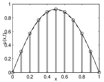Figure 2 shows the solution of (30) and the gap-tooth solution with $\Delta x=0.1$ , $\Delta t=1\cdot 10^{-3}$ and $h=0.01$ at time $t=0.02$ .

Difference with respect to finite differences.

We first compare the results of the gap-tooth scheme for (30) with those of a finite difference scheme for (31) with the same coarse parameters. We use a spatial interpolation/finite differences of order $k=2$ , with a coarse mesh of $\Delta x=0.1$ , resp. $\Delta x=0.05$ , for decreasing box sizes $h=0.04$ , $0.02$ , $0.01$ , $0.005$ , and for time-steps $\Delta t=\nu\Delta x^{2}$ , with $\nu=0.1$ , $0.2$ , $0.4$ . The results are shown in table 1 for $\Delta x=0.1$ and in table 2 for $\Delta x=0.05$ . They clearly show an $O(h^{2})$ decrease of the error initially, with a slow-down for smaller $h$ , due to the additional $O(\frac{\epsilon}{\Delta t})$ term. We also see that the decrease of convergence speed is affected by the time-step. The error decreases less rapidly for smaller $\nu$ , due to the additional error in each restriction step. Also note a smaller decrease for $\Delta x=0.05$ , because in this case $\Delta t$ is also smaller. Note that the difference with respect to finite differences does not depend dramatically on $\Delta t$ for this example, due to the absence of a reaction term (see theorem 4.4). By comparing tables 1 and 2, we also see that the difference between the gap-tooth scheme and the finite difference scheme is independent of $\Delta x$ , for fixed $h$ and $\nu$ .

	$\Delta t=0.1\Delta x^{2}$		$\Delta t=0.2\Delta x^{2}$		$\Delta t=0.4\Delta x^{2}$
	error	ratio	error	ratio	error	ratio
$h=0.04$	$5.4189\cdot 10^{-4}$		$5.3755\cdot 10^{-4}$		$5.3568\cdot 10^{-4}$
$h=0.02$	$1.4296\cdot 10^{-4}$	3.79	$1.3815\cdot 10^{-4}$	3.89	$1.3584\cdot 10^{-4}$	3.94
$h=0.01$	$4.3169\cdot 10^{-5}$	3.32	$3.8297\cdot 10^{-5}$	3.61	$3.5885\cdot 10^{-5}$	3.79
$h=0.005$	$1.8221\cdot 10^{-5}$	2.37	$1.3334\cdot 10^{-5}$	2.87	$1.0896\cdot 10^{-5}$	3.29

Table 1: Difference between the gap-tooth scheme for (30) and a finite difference scheme for (31) for order

k=2

and

\Delta x=0.1

at time

t=2\cdot 10^{-2}

	$\Delta t=0.1\Delta x^{2}$		$\Delta t=0.2\Delta x^{2}$		$\Delta t=0.4\Delta x^{2}$
	error	ratio	error	ratio	error	ratio
$h=0.04$	$5.6378\cdot 10^{-4}$		$5.5060\cdot 10^{-4}$		$5.4275\cdot 10^{-4}$
$h=0.02$	$1.7152\cdot 10^{-4}$	3.29	$1.5293\cdot 10^{-4}$	3.6	$1.5641\cdot 10^{-4}$	3.79
$h=0.01$	$7.2618\cdot 10^{-5}$	2.36	$5.3027\cdot 10^{-5}$	2.88	$4.3236\cdot 10^{-5}$	3.32
$h=0.005$	$4.7638\cdot 10^{-5}$	1.52	$2.8043\cdot 10^{-5}$	1.89	$1.8247\cdot 10^{-5}$	2.37

Table 2: Difference between the gap-tooth scheme for (30) and a finite difference scheme for (31) for order

k=2

and

\Delta x=0.05

at time

t=2\cdot 10^{-2}

The $O(\frac{\epsilon}{\Delta t})$ -term.

The evolution of the difference between the gap-tooth scheme and the finite difference scheme is shown in figure 3.

We see that we start with a constant error at time $t=0$ due to the averaging of the initial condition. Note that this error is not important if one compares to the exact averaged solution $U(x,t)$ . It is an artifact of comparing to the homogenized equation instead of the effective equation. However, if $u_{0}(x,t)$ evolves according to (31), $U(x,t)=\mathcal{S}_{h}(u_{0})(x,t)$ evolves according to the same equation. Therefore, we can eliminate the $O(h^{2})$ term, by comparing to $U(x,t)$ instead of $u_{0}(x,t)$ . This allows us to show that the stagnation in tables 1 and 2 is really $\epsilon$ -dependent. We compare the results of the gap-tooth scheme and the finite difference scheme of order $2$ for $\Delta x=0.05$ and $h=0.02$ at time $t=2\cdot 10^{-2}$ . We first keep $\Delta t=1\cdot 10^{-3}$ fixed, and vary $\epsilon=1\cdot 10^{-3}$ , $2\cdot 10^{-3}$ , $4\cdot 10^{-3}$ . Subsequently, we fix $\epsilon=1\cdot 10^{-3}$ , and vary $\Delta t=0.5\cdot 10^{-3}$ , $1\cdot 10^{-3}$ , $2\cdot 10^{-3}$ . The results are shown in table 3. For this simple example, the error decreases quadratically with $\epsilon$ , because the error constant of the $O(\epsilon)$ term is zero. If we combine the results from both tables, we clearly see a decrease in error according to $O(\frac{\epsilon^{2}}{\Delta t})$ for this example.

	error	ratio
$\epsilon=4\cdot 10^{-3}$	$3.0574\cdot 10^{-4}$
$\epsilon=2\cdot 10^{-3}$	$7.6239\cdot 10^{-5}$	4.01
$\epsilon=1\cdot 10^{-3}$	$1.9710\cdot 10^{-5}$	3.87

	error	ratio
$\Delta t=0.5\cdot 10^{-3}$	$3.9304\cdot 10^{-5}$
$\Delta t=1\cdot 10^{-3}$	$1.9710\cdot 10^{-5}$	1.99
$\Delta t=2\cdot 10^{-3}$	$9.9133\cdot 10^{-6}$	1.99

Table 3: Left: Difference between the results of the gap-tooth scheme and the forward Euler/spatial finite difference scheme of order

2

for

\Delta x=0.05

\Delta t=1\cdot 10^{-3}

h=0.02

, at time

t=2\cdot 10^{-2}

, for

\epsilon=1\cdot 10^{-3}

2\cdot 10^{-3}

4\cdot 10^{-3}

after subtracting the

O(h^{2})

error in the initial data. Right: Difference for

\epsilon=1\cdot 10^{-3}

\Delta t

varying.

Error with respect to solution of the homogenized problem.

We also show the error with respect to the exact solution of the homogenized problem. For this purpose, we compute the homogenized solution with a second order finite difference approximation in space with $\delta x=1\cdot 10^{-5}$ and implicit Euler time-steps with $\delta t=5\cdot 10^{-7}$ . The gap-tooth scheme is used with box width $h=0.005$ , $\Delta x=0.2$ , $0.1$ and $\Delta t=\nu\Delta x^{k}$ with $\nu=0.4$ and order $k=2$ . We compare the gap-tooth and the finite difference solution to the exact solution for the homogenized equation at time $t=2\cdot 10^{-2}$ . The results are shown in figure 4. It is clear that the error is similar to that of the finite difference scheme. Note however that the errors will increase when the $O(h^{2})$ and $O({\epsilon}{\Delta t})$ terms in the error become dominant.

Higher order discretizations in space.

We repeat the same experiment for a gap-tooth scheme of order $k=4$ , which we compare to a fourth order spatial finite difference approximation, with an explicit Euler time-step. As parameters, we choose $\Delta x=0.1$ , $0.05$ and $\Delta t=\nu\Delta x^{4}$ , with $\nu=0.4$ and $h=0.01$ . In order to view the $O(\Delta x^{4})$ behaviour, we need to choose $\Delta t$ correspondingly small, which will affect convergence through the $O(\frac{\epsilon}{\Delta t})$ term. The results are shown in figure 5. It is clear for $\Delta x=0.1$ that the scheme approximates the fourth order scheme. In this case, the time-step $\Delta t=4\cdot 10^{-5}$ . However, for $\Delta x=0.05$ , $\Delta t=2.5\cdot 10^{-6}$ , the error is already completely dominated by the $O(\frac{\epsilon}{\Delta t})$ term.

5.2 Periodic diffusion with non-linear reaction

As a second example, we consider the following reaction-diffusion equation

\frac{\partial}{\partial t}u_{\epsilon}(x,t)=\frac{\partial}{\partial x}\left(a(\frac{x}{\epsilon})\frac{\partial}{\partial}u_{\epsilon}(x,t)\right)+u_{\epsilon}(x,t)(1-\frac{u_{\epsilon}(x,t)}{b(x)}),

(32)

where $a(\frac{x}{\epsilon})=1.1+\sin(2\pi\frac{x}{\epsilon})$ as in section 5.1, and $b(x)=\sin(2\pi x)+1.2$ . This model can be interpreted as a one-species logistic growth model with macroscopically varying capacity $b(x)$ and a rapidly oscillating diffusion coefficient $a(\frac{x}{\epsilon})$ . We choose periodic boundary conditions and a constant initial condition, $u^{0}(x)=0.7$ . The corresponding homogenized problem is given by

\frac{\partial}{\partial t}u_{\epsilon}(x,t)=\frac{\partial}{\partial x}\left(a^{*}\frac{\partial}{\partial}u_{\epsilon}(x,t)\right)+u_{\epsilon}(x,t)(1-\frac{u_{\epsilon}(x,t)}{b(x)}),

(33)

with $a^{*}\approx 0.45825686$ . Figure 6 shows the solution of (32), as well as the result of a gap-tooth simulation with parameters $\Delta x=0.05$ , $\Delta t=1\cdot 10^{-3}$ , $h=0.01$ for $t=2\cdot 10^{-2}$ . The reference solution was computed with second order spatial finite differences and an implicit Euler time-stepper, with $\delta x=1\cdot 10^{-5}$ and $\delta t=5\cdot 10^{-7}$ .

In contrast to the example in section 5.1, there will be also an $O(\Delta t)$ difference between the gap-tooth solution and the finite difference scheme. To show this, we compare the gap-tooth scheme with $\Delta x=0.1$ and $\Delta t=\nu\Delta x^{2}$ with a finite difference scheme for the homogenized equation with the same coarse parameters for $\nu=0.05$ , $0.1$ , $0.2$ , $0.4$ . We did this for box width $h=0.005$ and $0.01$ . The results are shown in table 4.

	$h=0.005$		$h=0.01$
	error	ratio	error	ratio
$\Delta t=4\cdot 10^{-3}$	$1.3842\cdot 10^{-4}$		$1.3929\cdot 10^{-4}$
$\Delta t=2\cdot 10^{-3}$	$7.9135\cdot 10^{-5}$	1.75	$7.9792\cdot 10^{-5}$	1.75
$\Delta t=1\cdot 10^{-3}$	$5.1103\cdot 10^{-5}$	1.55	$5.1496\cdot 10^{-5}$	1.55
$\Delta t=5\cdot 10^{-4}$	$3.8014\cdot 10^{-5}$	1.34	$3.7959\cdot 10^{-5}$	1.36

Table 4: Difference between the gap-tooth scheme for (30) and a finite difference scheme for (31) for order

k=2

and

\Delta x=0.05

at time

t=2\cdot 10^{-2}

¿From this table we see that a smaller time-step indeed gives a smaller difference with respect to the corresponding finite difference scheme. However, we do not observe the ratio $2$ . We can show that this is due to the interference of the $O(\frac{\epsilon}{\Delta t})$ -term. Indeed, if we replace the microscopic problem inside each box with the homogenized problem with Neumann boundary conditions, the $O(\frac{\epsilon}{\Delta t})$ -term vanishes. The result is shown in table 5.

	$h=0.005$		$h=0.01$
	error	ratio	error	ratio
$\Delta t=4\cdot 10^{-3}$	$1.0812\cdot 10^{-4}$		$1.0982\cdot 10^{-4}$
$\Delta t=2\cdot 10^{-3}$	$4.9371\cdot 10^{-5}$	2.19	$5.1135\cdot 10^{-5}$	2.15
$\Delta t=1\cdot 10^{-3}$	$2.1459\cdot 10^{-5}$	2.3	$2.3411\cdot 10^{-5}$	2.18
$\Delta t=5\cdot 10^{-4}$	$8.1325\cdot 10^{-5}$	2.63	$1.0492\cdot 10^{-5}$	2.23

Table 5: Difference between the gap-tooth scheme for (30) and a finite difference scheme for (31) for order

k=2

and

\Delta x=0.05

at time

t=2\cdot 10^{-2}

We see that the decrease of convergence speed indeed disappears. The observed ratios are slightly larger than 2, due to the interference with the $O(h^{2})$ term due to averaging, which is opposite in sign.

5.3 Rough non-periodic (random) diffusion

With this example, we illustrate that the scheme can also be used to simulate systems with rough coefficients, which are correlated on a length scale $\epsilon$ . We use the same example as Abdulle and E [1], who constructed it to demonstrate the behaviour of the heterogeneous multi-scale method. We first take a uniformly distributed random signal $s(x)$ in $[0.1,1.1]$ , with $x\in[0,1]$ . We discretize the interval $[0,1]$ in $N$ equidistant points $x_{i}$ , and define a correlation kernel $g^{\epsilon}(x)$ , such that

g^{\epsilon}(0)=\frac{1}{\epsilon},\qquad g^{\epsilon}(x)=0\text{ if }x\notin(-\frac{\epsilon}{2},\frac{\epsilon}{2}),\qquad\int_{-\frac{\epsilon}{2}}^{\frac{\epsilon}{2}}g^{\epsilon}(x)\mathrm{d}x=1.

Here, we choose $g^{\epsilon}(x)=\frac{1}{\epsilon}(1-\sin(\frac{2\pi x}{\epsilon}))$ , $x\in(-\frac{\epsilon}{2},\frac{\epsilon}{2})$ . We then define the rough diffusion coefficient in the discretization points as

a^{\epsilon}(x_{i})=(g^{\epsilon}*s)(x_{i})=\int_{-\frac{\epsilon}{2}}^{\frac{\epsilon}{2}}g^{\epsilon}(x_{i}-\xi)s(\xi)\mathrm{d}\xi.

We then consider the diffusion equation

\frac{\partial}{\partial t}u_{\epsilon}(x,t)=\frac{\partial}{\partial x}\left(a^{\epsilon}(x)\frac{\partial}{\partial x}u_{\epsilon}(x,t)\right),

with $a^{\epsilon}(x)$ constructed as above. Note that this is a deterministic problem once the diffusion coefficient is obtained. We consider only one realization of the diffusion coefficient field. Here, we can approximate the effective behaviour by averaging in space; in [20], one had to average over many (shifted) initial conditions.

We compute the solution with $N=20001$ and $\epsilon=1\cdot 10^{-3}$ , and we compare this to a gap-tooth solution with $h=5\cdot 10^{-3}$ . As an initial condition, we take $u_{\epsilon}(x,0)=1-4(x-0.5)^{2}$ , with homogeneous Dirichlet boundary conditions. Figure 7 shows the diffusion coefficient and the reference and gap-tooth solutions.

We compute the solution for this problem with an increasing number of boxes, where $\nu=0.2$ is fixed and $\Delta t=\nu\Delta x^{2}$ . The error is shown in table 6.

	error
$\Delta x=2\cdot 10^{-1}$	$1.0283\cdot 10^{-2}$
$\Delta x=1\cdot 10^{-1}$	$8.1064\cdot 10^{-3}$
$\Delta x=5\cdot 10^{-2}$	$7.4622\cdot 10^{-3}$
$\Delta x=2.5\cdot 10^{-2}$	$1.4028\cdot 10^{-3}$

Table 6: Difference between the gap-tooth scheme with

h=5\cdot 10^{-3}

and the reference solution at time

t=2\cdot 10^{-2}

for increasing level of discretization.

We see that the error decreases when more boxes are inserted. Note that, due to the roughness of the signal, it is difficult to draw conclusions on the convergence rate, and to determine good parameter values for the gap-tooth scheme. E.g. the length over which the gradient is averaged at the end points of each box is no longer uniquely defined, since the small scale $\epsilon$ is only a correlation length.

6 Avoiding the algebraic constraint

We recall that the gap-tooth scheme, as presented above, performs the simulations inside each box using an algebraic constraint, ensuring that the initial macroscopic gradient is preserved at the boundary of each box over the time-step $\Delta t$ . If our goal is to accelerate time-integration using an existing microscopic code, this constraint may require us to alter this code, so as to impose this macroscopically-inspired constraint. This may be impractical (e.g. if the macroscopic gradient has to be estimated), undesirable (e.g. if the development of the code is expensive and time-consuming) or even impossible (e.g. if the microscopic code is a legacy code).

Generally, a given microscopic code allows us to run with a set of pre-defined boundary conditions. It is highly non-trivial to impose macroscopically inspired boundary conditions on such microscopic codes, see e.g. [16] for a control-based strategy. This can be circumvented by introducing buffer regions at the boundary of each small box, which shield the dynamics within the computational domain of interest from boundary effects during a short time interval. One then uses the microscopic code with its built-in boundary conditions [21].

6.1 The gap-tooth scheme with buffers

We note that, for a correct simulation, the only crucial issue is that the detailed system in each box should evolve as if it were embedded in a larger domain. This can be effectively accomplished by introducing a larger box of size $H>>h$ around each macroscopic mesh point, but still only use (for macro-purposes) the evolution over the smaller, “inner” box. This is illustrated in figure 8. Lifting and evolution (using arbitrary outer boundary conditions) are performed in the larger box; yet the restriction is done by taking the average of the solution over the inner, small box. The goal of the additional computational domains, the buffers, is to buffer the solution inside the small box from outer boundary effects. This can be accomplished over short enough times, provided the buffers are large enough; analyzing the method is tantamount to making these statements quantitative.

The idea of using a buffer region was also used in the multi-scale finite element method (oversampling) of Hou [10] to eliminate the boundary layer effect; also Hadjiconstantinou makes use of overlap regions to couple a particle simulator with a continuum code [9]. If the microscopic code allows a choice of different types of “outer” microscopic boundary conditions, selecting the size of the buffer may also depend on this choice.

6.2 Damping factors

Here, we show that we can study the gap-tooth scheme (with buffers) through its numerically obtained damping factors, i.e. by estimating the eigenvalues of its linearization. Integration with nearby coarse initial conditions is used to estimate matrix-vector products of the linearization of the coarse time- $\Delta t$ map with known perturbation vectors; these are integrated in matrix-free iterative methods such as Arnoldi eigensolvers. For the diffusion homogenization problem (30), we show that the eigenvalues of the gap-tooth scheme are approximately the same as those of the corresponding finite difference scheme for (31). When we impose Dirichlet boundary conditions at the boundary of the buffers, we show that the scheme converges to the standard gap-tooth scheme for increasing buffer size.

Convergence results are typically established by proving consistency and stability. If one can prove that the error in each time step can be made arbitrarily small by refining the spatial and temporal mesh size, and that an error made at time $t_{n}$ does not get amplified in future time-steps, one has proved convergence. This requires the solution operator to be stable as well. In the absence of explicit formulas, one can examine the damping factors of the time-stepper. If, for decreasing mesh sizes, all (finitely many) eigenvalues and eigenfunctions of the time-stepper converge to the dominant eigenvalues and eigenfunctions of the time evolution operator, one expects the solution of the scheme to converge to the true solution of the evolution problem.

Consider equation (31) with Dirichlet boundary conditions $u(0,t)=0$ and $u(1,t)$ , and denote its solution at time $t$ by the time evolution operator

u(x,t)=s(u_{0}(x);t),

(34)

We know that

s(\sin(m\pi x);t)=\mathrm{e}^{-(m\pi)^{2}t}\sin(m\pi x),\qquad m\in\mathbb{N}.

Therefore, if we consider the time evolution operator over a fixed time $\bar{t}$ , $s(\cdot,\bar{t})$ , then this operator has eigenfunctions $\sin(m\pi x)$ , with resp. eigenvalues

\lambda_{m}=\mathrm{e}^{-{(m\pi)}^{2}\bar{t}}.

(35)

A good (finite difference) scheme approximates well all eigenvalues whose eigenfunctions can be represented on the given mesh. We choose $\bar{t}$ as a multiple of $\Delta t$ for convenience.

Since the operator defined in (34) is linear, the numerical time integration is equivalent to a matrix-vector product. Therefore, we can compute the eigenvalues using matrix-free linear algebra techniques, even for the gap-tooth scheme, for which it might not even be possible to obtain a closed expression for the matrix. Note that this idea is general; here we use it as a tool to study the effect of the buffer size on convergence of the gap-tooth scheme. However, although this analysis gives us an indication about the quality of the scheme, it is by no means a proof of convergence.

6.3 Numerical results

We illustrate this idea by computing the eigenvalues of the gap-tooth scheme of order $k=2$ , applied to (30). In this case, we know from section 4 that these eigenvalues should approximate the eigenvalues of a finite difference scheme on the same mesh. As method parameters, we choose $\Delta x=0.05$ , $h=5\cdot 10^{-3}$ , $\Delta t=2.5\cdot 10^{-4}$ for a time horizon $\bar{t}=4\cdot 10^{-3}$ , which corresponds to 16 gap-tooth steps. Inside each box, we use a finite difference scheme of order $2$ with $\delta x=1\cdot 10^{-5}$ and an implicit Euler time-step of $5\cdot 10^{-7}$ . We compare these eigenvalues to those of the finite difference scheme with $\Delta x=0.05$ and $\Delta t=2.5\cdot 10^{-4}$ , and with the dominant eigenvalues of the reference solution (a finite difference approximation with $\Delta x=1\cdot 10^{-5}$ , $\Delta t=5\cdot 10^{-7}$ and implicit Euler time-stepping). The result is shown in figure 9.

We now introduce a buffer region of size $H$ , and we impose Dirichlet boundary conditions at the outer boundary of the buffer region. Lifting is done in identically the same way as for the gap-tooth scheme without buffers; we only use (9) as the initial condition in the larger box $[x_{i}-\frac{H}{2},x_{i}+\frac{H}{2}]$ . We compare the eigenvalues again with the equivalent finite difference scheme and the exact solution, for increasing sizes of the buffer box $H$ . Figure 10 shows that, as $H$ increases, the eigenvalues of the scheme converge to those of the original gap-tooth scheme. We see that, in this case, we would need a buffer of size $H=4\cdot 10^{-2}$ , i.e. 80% of the original domain, for a good approximation of the damping factors. It is possible to decrease the buffer size by decreasing $\Delta t$ , which results in more re-initializations.

7 Conclusions

We described the gap-tooth scheme for the numerical simulation of multi-scale problems. This scheme simulates the macroscopic behaviour over a macroscopic domain when only a microscopic model is explicitly available. We analyzed the convergence of this scheme for a parabolic homogenization problem with non-linear reaction.

We showed that our method approximates a finite difference scheme of arbitrary (even) order for the homogenized equation when we appropriately constrain the microscopic problem in the boxes, and illustrated this theoretical result with numerical tests on several model problems. Our analysis revealed that the presence of microscopic scales, combined with the requirement that the macroscopic gradient does not change over one gap-tooth time-step $\Delta t$ , introduces an error term that grows with decreasing $\Delta t$ , which is not optimal.

We also demonstrated that it is possible to obtain a convergent scheme without constraining the microscopic code, by introducing buffers that shield over relatively short time intervals the dynamics inside each box from boundary effects. It is possible, even without analytic formulas, to study the properties of the gap-tooth scheme and generalizations through the damping factors of the resulting coarse time- $\Delta t$ map. In a forthcoming paper, we will use these damping factors to study the the trade-off between the effort required to impose a particular type of boundary conditions and the efficiency gain due to smaller buffer sizes and/or longer possible time-steps before reinitialization.

The time-stepper as constructed in this paper will allow us to perform simulations of the effective behaviour of a microscopic system over macroscopic space and macroscopic time (when combined with projective integration), or to perform tasks as bifurcation analysis or coarse control (when coupled to time-stepper based bifurcation codes).

Acknowledgments

The authors thank Sabine Attinger and Petros Koumoutsakos for organizing the Summer School in Multi-scale Modeling and Simulation in Lugano, and the participants for many fruitful discussions. Giovanni Samaey is a Research Assistant of the Fund for Scientific Research - Flanders. This work has been partially supported by grant IUAP/V/22 and by the Fund of Scientific Research through Research Project G.0130.03 (GS, DR), and an NSF/ITR grant and AFOSR Dynamics and Control, Dr. B. King (IGK).

References

[1] A. Abdulle and W. E. Finite difference heterogeneous multi-scale method for homogenization problems. Journal of Computational Physics, 0(0):1–25, 2003.
[2] G. Allaire. Homogenization and two-scale convergence. SIAM Journal of Mathematical Analysis, 23(6):1482–1518, 1992.
[3] A. Bensoussan, J.L. Lions, and G. Papanicolaou. Asymptotic analysis of periodic structures, volume 5 of Studies in Mathematics and its Applications. North-Holland, Amsterdam, 1978.
[4] D. Cioranescu and P. Donato. An introduction to homogenization. Oxford University Press, 1999.
[5] W. E and B. Engquist. The heterogeneous multi-scale methods. Comm. Math. Sci., 1(1):87–132, 2003.
[6] C.W. Gear and I.G. Kevrekidis. Constraint-defined manifolds: a legacy code approach to low-dimensional computation. J. Sci. Comp., 2003. submitted.
[7] C.W. Gear and I.G. Kevrekidis. Projective methods for stiff differential equations: problems with gaps in their eigenvalue spectrum. SIAM Journal of Scientific Computation, 24(4):1091–1106, 2003. Can be obtained as NEC Report 2001-029, http://www.neci.nj.nec.com/homepages/cwg/projective.pdf.
[8] C.W. Gear, J. Li, and I.G. Kevrekidis. The gap-tooth method in particle simulations. Physics Letters A, 316:190–195, 2003. Can be obtained as physics/0303010 at arxiv.org.
[9] N.G. Hadjiconstantinou. Hybrid atomistic-continuum formulations and the moving contact-line problem. Journal of Computational Physics, 154:245–265, 1999.
[10] T.Y. Hou and X.H. Wu. A multiscale finite element method for elliptic problems in composite materials and porous media. Journal of Computational Physics, 134:169–189, 1997.
[11] T.Y. Hou and X.H. Wu. Convergence of a multiscale finite element method for elliptic problems with rapidly oscillating coefficients. Mathematics of Computation, 68(227):913–943, 1999.
[12] G. Hummer and I.G. Kevrekidis. Coarse molecular dynamics of a peptide fragment: free energy, kinetics and long-time dynamics computations. Journal of Chemical Physics, 118(23):10762–10773, 2003. Can be obtained as physics/0212108 at arxiv.org.
[13] I.G. Kevrekidis. Coarse bifurcation studies of alternative microscopic/hybrid simulators. Plenary lecture, CAST Division, AIChE Annual Meeting, Los Angeles, 2000. Slides can be obtained from http://arnold.princeton.edu/~yannis/.
[14] I.G. Kevrekidis, C.W. Gear, J.M. Hyman, P.G. Kevrekidis, O. Runborg, and C. Theodoropoulos. Equation-free multiscale computation: enabling microscopic simulators to perform system-level tasks. Comm. Math. Sciences, 2002. in press. Can be obtained as physics/0209043 from arxiv.org.
[15] J. Li, P.G. Kevrekidis, C.W. Gear, and I.G. Kevrekidis. Deciding the nature of the “coarse equation” through microscopic simulations: the baby-bathwater scheme. SIAM Multiscale modeling and simulation, 1(3):391–407, 2003.
[16] J. Li, D. Liao, and S. Yip. Imposing field boundary conditions in MD simulation of fluids: optimal particle controller and buffer zone feedback. Mat. Res. Soc. Symp. Proc, 538:473–478, 1998.
[17] A.G. Makeev, D. Maroudas, and I.G. Kevrekidis. Coarse stability and bifurcation analysis using stochastic simulators: kinetic Monte Carlo examples. Journal of Chemical Physics, 116:10083–10091, 2002.
[18] A.G. Makeev, D. Maroudas, A.Z. Panagiotopoulos, and I.G. Kevrekidis. Coarse bifurcation analysis of kinetic Monte Carlo simulations: a lattice-gas model with lateral interactions. Journal of Chemical Physics, 117(18):8229–8240, 2002.
[19] A.M. Matache, I. Babuska, and C. Schwab. Generalized p-FEM in homogenization. Numerische Mathematik, 86(2):319–375, 2000.
[20] O. Runborg, C. Theodoropoulos, and I.G. Kevrekidis. Effective bifurcation analysis: a time-stepper based approach. Nonlinearity, 15:491–511, 2002.
[21] G. Samaey, I.G. Kevrekidis, and D. Roose. Damping factors for the gap-tooth scheme. Lecture Notes in Computational Science and Engineering. Springer, 2003. Submitted. Can be obtained as physics/0310014 at arxiv.org.
[22] C. Schwab and A.M. Matache. Generalized FEM for homogenization problems, volume 20 of Lecture Notes in Computational Science and Engineering, pages 197–238. Springer-Verlag, 2002.
[23] S. Setayeshar, C.W. Gear, H.G. Othmer, and I.G. Kevrekidis. Application of coarse integration to bacterial chemotaxis. SIAM Multiscale modelling and simulation, 2003. Submitted.
[24] C.I. Siettos, A. Armaou, A.G. Makeev, and I.G. Kevrekidis. Microscopic/stochastic timesteppers and coarse control: a kinetic Monte Carlo example. AIChE J., 49(7):1922–1926, 2003. can be obtained as nlin.CG/0207017 at arxiv.org.
[25] C.I. Siettos, M.D. Graham, and I.G. Kevrekidis. Coarse brownian dynamics for nematic liquid crystals: bifurcation, projective integration and control via stochastic simulation. can be obtained as cond-mat/0211455 at arxiv.org, 2003.
[26] C. Theodoropoulos, Y.H. Qian, and I.G. Kevrekidis. Coarse stability and bifurcation analysis using time-steppers: a reaction-diffusion example. In Proc. Natl. Acad. Sci., volume 97, 2000.
[27] C. Theodoropoulos, K. Sankaranarayanan, S. Sundaresan, and I.G. Kevrekidis. Coarse bifurcation studies of bubble flow Lattice-Boltzmann simulations. Chem. Eng. Sci., 2003. can be obtained as nlin.PS/0111040 from arxiv.org.

$\displaystyle\left\\|U(x,t)-u_{0}(x,t)\right\\|$	$\displaystyle=$	$\displaystyle\left\\|\frac{1}{h}\int_{x-\frac{h}{2}}^{x+\frac{h}{2}}u(\xi,t)\mathrm{d}\xi-u_{0}(x,t)\right\\|$
	$\displaystyle\leq$	$\displaystyle\left\\|\frac{1}{h}\int_{x-\frac{h}{2}}^{x+\frac{h}{2}}u_{0}(\xi,t)\mathrm{d}\xi-u_{0}(x,t)\right\\|$
		$\displaystyle+\epsilon\left\\|\int_{x-\frac{h}{2}}^{x+\frac{h}{2}}u_{1}(\xi,\frac{\xi}{\epsilon},t)-\theta_{1}(\xi,\frac{\xi}{\epsilon},t)\mathrm{d}\xi\right\\|+O(\epsilon^{2})$
	$\displaystyle\leq$	$\displaystyle\frac{h^{2}}{24}\left\|\frac{\partial^{2}}{\partial x^{2}}u_{0}(x,t)\right\|+C_{2}\epsilon$
	$\displaystyle\leq$	$\displaystyle\frac{h^{2}}{24}\max_{x\in[0,1]}\left\|\frac{\partial^{2}}{\partial x^{2}}u_{0}(x,t)\right\|+C_{2}\epsilon$

$\displaystyle\left\\|\bar{U}^{n+1}_{i}-\hat{U}_{i}^{n+1}\right\\|$
	$\displaystyle=$	$\displaystyle\left\\|G_{i}^{n}\Delta t-\frac{1}{h}\int_{t_{n}}^{t_{n}+\Delta t}\int_{x_{i}-\frac{h}{2}}^{x_{i}+\frac{h}{2}}g(\tilde{u}_{0}^{i}(\xi,t))\mathrm{d}\xi\mathrm{d}t\right\\|$
	$\displaystyle\leq$	$\displaystyle\left\\|\frac{1}{h}\int_{x_{i}-\frac{h}{2}}^{x_{i}+\frac{h}{2}}\left(g\left(u(\xi,t_{n})\right)\Delta t-\int_{t_{n}}^{t_{n}+\Delta t}g\left(u(\xi,t)\right)\mathrm{d}t\right)\mathrm{d}\xi\right\\|$
	$\displaystyle+$	$\displaystyle\left\\|\frac{1}{h}\int_{x_{i}-\frac{h}{2}}^{x_{i}+\frac{h}{2}}\int_{t_{n}}^{t_{n}+\Delta t}\left(g\left(u(\xi,t)\right)-g\left(\tilde{u}_{0}^{i}(\xi,t)\right)\right)\mathrm{d}t\mathrm{d}\xi\right\\|$

$\displaystyle\left\\|U_{i}^{n}-u_{0}(x_{i},t_{n})\right\\|$
	$\displaystyle\leq$	$\displaystyle\left\\|U_{i}^{n}-\bar{U}_{i}^{n}\right\\|+\left\\|\bar{U}_{i}^{n}-U(x_{i},t_{n})\right\\|+\left\\|U(x_{i},t_{n})+u_{0}(x_{i},t_{n})\right\\|$
	$\displaystyle\leq$	$\displaystyle\left\\|U_{i}^{n}-\bar{U}_{i}^{n}\right\\|+C_{5}\Delta x^{k}+C_{6}\Delta t+C_{1}h^{2}+C_{2}\epsilon.$

$\displaystyle\left\\|U^{n}-\bar{U}^{n}\right\\|$	$\displaystyle=$	$\displaystyle\left\\|S_{k}(U^{n-1},t_{n-1}+\Delta t)-\bar{S}_{k}(\bar{U}^{n-1},t_{n-1}+\Delta t)\right\\|$
	$\displaystyle\leq$	$\displaystyle\left\\|S_{k}(U^{n-1},t_{n-1}+\Delta t)-\bar{S}_{k}(U^{n-1},t_{n-1}+\Delta t)\right\\|$
	$\displaystyle+$	$\displaystyle\left\\|\bar{S}_{k}(U^{n-1},t_{n-1}+\Delta t)-\bar{S}_{k}(\bar{U}^{n-1},t_{n-1}+\Delta t)\right\\|$
	$\displaystyle\leq$	$\displaystyle\left\\|A_{k}(U^{n-1}-\bar{U}^{n-1})\right\\|+C_{3}\epsilon+C_{4}\Delta t^{2},$

The gap-tooth scheme for homogenization problems

Abstract

1 Introduction

2 The gap-tooth scheme

Boundary constraints.

Initial conditions.

The algorithm.

Microscopic simulators.

3 Model homogenization problem

3.1 Standard homogenization theory

3.2 Homogenization and averaging

Lemma 3.1.

Lemma 3.2.

Proof.

4 Convergence results

Lemma 4.1.

Lemma 4.2.

Proof.

Lemma 4.3.

Proof.

Theorem 4.4 (Local error).

Proof.

Theorem 4.5.

Proof.

5 Numerical results

5.1 Periodic diffusion coefficient without reaction

Difference with respect to finite differences.

The O⁡(ϵΔ​t)O(\frac{\epsilon}{\Delta t})-term.

Error with respect to solution of the homogenized problem.

Higher order discretizations in space.

5.2 Periodic diffusion with non-linear reaction

5.3 Rough non-periodic (random) diffusion

6 Avoiding the algebraic constraint

6.1 The gap-tooth scheme with buffers

6.2 Damping factors

6.3 Numerical results

7 Conclusions

Acknowledgments

References

The $O(\frac{\epsilon}{\Delta t})$ -term.