Two dimensional modulational instability in photorefractive media
Abstract
We study theoretically and experimentally the modulational instability of broad optical beams in photorefractive nonlinear media. We demonstrate the impact of the anisotropy of the nonlinearity on the growth rate of periodic perturbations. Our findings are confirmed by experimental measurements in a strontium barium niobate photorefractive crystal.
pacs
42.65.Hw, 42.65.JxA plane wave propagating in a medium with focusing nonlinearity is unstable with respect to the generation of small scale filaments BesTal. This so called modulational instability (MI) phenomenon, has been extensively studied because of its importance as a factor limiting the propagation of high power beams. Filamentation may also be identified as the first stage in the development of turbulent fluctuations in the transverse profile of a laser beamzak92. In addition, MI is often considered as a precursor for the formation of spatial and/or temporal optical solitons. As far as optics is concerned, MI has been studied in media with various mechanisms of nonlinear response including cubic BesTal, quadratic MI_SHG, nonlocal nonlocal1; nonlocal2 and inertial MI_slow; MI_incoherent types of nonlinearity. Importantly, MI is not restricted to nonlinear optics but has also been studied in many other nonlinear systems including fluids fluids, plasmas plasma and matter waves BEC.
In the context of optical beam propagation in nonlinear materials MI has usually been considered in media with spatially isotropic nonlinear properties. Recently a great deal of theoretical and experimental efforts have been devoted to studies of nonlinear optical effects and soliton formation in photorefractive crystals PR1; PR2; PR3. While these media exhibit strong nonlinearity at very low optical power their nonlinear response is inherently anisotropic zapra. The anisotropy causes a number of observable effects including astigmatic self-focusing of optical beams astigmatism, elliptically shaped solitary solutionszams, geometry-sensitive interactions of solitons ks, and fixed optical pattern orientation mamsaflinear.
Several previous studies of MI in the context of photorefractive media were limited to a 1-dimensional geometry where the anisotropy is absent MI_PR1; MI_PR2; MI_PR3, and the physics is similar to the standard saturable nonlinearity saturable. On the other hand, in a real physical situation where one deals with finite sized beams, the anisotropic aspects of the photorefractive nonlinear response are expected to play a significant role. Some previous work msz1; zamspra2 already indicated the importance of anisotropy in the transversal break-up of broad beams propagating in biased photorefractive crystals. However, no detailed analysis of this phenomenon was carried out. In this paper we study the MI of optical beams in photorefractive media taking into account the full 2-dimensional anisotropic model of the photorefractive nonlinearity.
Time independent propagation of an optical beam in a nonlinear medium with a weakly varying index of refraction is governed by the parabolic equation
| (1) |
Here and are transverse and axial coordinates, is the wavelength in vacuum, is the speed of light, and is the refractive index, with the spatially uniform background index, and the spatially varying nonlinear increment.
In the case of a photorefractive screening nonlinearity the optical beam propagates through a photorefractive crystal externally biased with a DC electric field. The beam excites charges which after migrating due to diffusion and drift in the applied field, are subsequently trapped by impurity or defect centers. The effective nonlinearity (refractive index change) is proportional to the low frequency electric field created by light induced charge redistribution PR1; PR2; zapra. In the situation of interest here where the optical field is linearly polarized along which coincides with the crystalline axis the nonlinear increment to the refractive index is given by with the relevant component of the electro-optic tensor, and the component of the low frequency electric field in the medium.
It is convenient to describe the nonlinear material response in terms of the quasi-static potential induced by the optical field. As shown in the appendix the resulting set of dimensionless equations is
| (2) | |||
| (3) |
where The coordinates and variables have been normalized using the scalings given in the appendix with the addition of with
Equation (3) describes the most general situation when the electrostatic potential in the crystal is induced by two distinct transport mechanisms: drift of charges in the biasing DC field plus photogalvanic field and their diffusion. The relative strength of the diffusion and drift terms is determined by the dimensionless parameter
The diffusion contribution which leads to spatially asymmetric stimulated scattering dominates at large transverse wavenumbers of order On the other hand the drift terms give the dominant contribution to the spatially symmetric MI which is prominent at much smaller transverse wavenumbers. Thus the term proportional to in Eq. (3) is often neglected when studying MI.
The initial linear stage of the filamentation instability may be investigated by putting
| (4) |
where represents the growth rate of the perturbation characterized by the transverse wavevector , and frequency detuning .
The steady state solution to Eq. (3) in the one dimensional plane wave limit with is where is the amplitude of the plane wave which is assumed to vanish for . It is therefore convenient to renormalize the potential as so that the equations of motion become
| (5) | |||
| (6) |
with The ansatz (4) then gives which provides a continuous transition to the 1D solution.
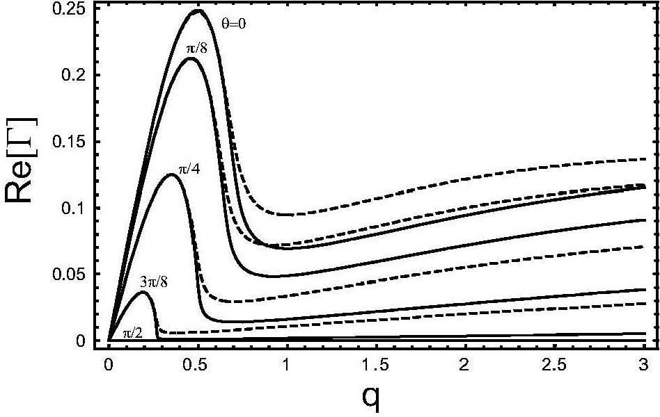
Solving the linear problem defined by Eqs. (4-6) gives the dispersion relation
| (7) |
where with the static dielectric tensor component along and the angle of with respect to the axis. In the limit of a single transverse dimension () without diffusion Eq.(7) reduces to the formula for the growth rate in saturable nonlinear media MI_slow; saturable.
The instability growth rate is given by . In Fig.1 we show the growth rate as a function of the spatial frequency for a few values of the angle using parameters characteristic of a photorefractive crystal as given in the appendix. The growth rate depends strongly on the angular orientation of the initial perturbation. In particular, it always attains the largest value when the wave vector of the perturbation coincides with the direction of the applied electric field (). As departs from zero the amplification of the perturbation decreases, and the growth rate becomes less strongly peaked at small . The growth rate is an even function of provided and inspection of Eq. (7) shows that it falls of for large as Interestingly Eq.(7) predicts there is no instability for perturbations with wave vectors perpendicular to the direction of the applied field.
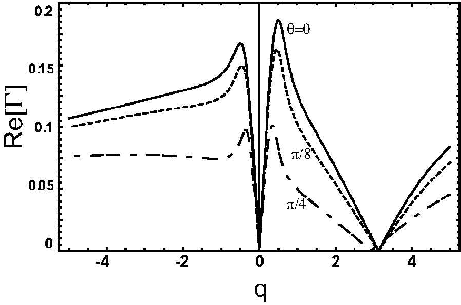
When the perturbation is frequency shifted with respect to the plane wave the growth rate becomes an asymmetric function of This is shown in Fig. 2 for Positive in the figure corresponds to the direction of a plane wave that experiences two-wave mixing gain. We see that the growth rate has several maxima as a function of in the presence of a frequency shift.
Finally we note that the angular dependence takes on a simple form in the small limit where the diffusion contribution can be neglected. Putting in (7) and assuming no frequency shift so we obtain
| (8) |
This latter expression shows clearly the decline of the instability growth rate with increasing angle away from the axis.


In order to verify the reliability of the linear approximation discussed above we resorted to numerical analysis of the full 2-dimensional model governing propagation of optical beams in a photorefractive medium Eqs. (2,3). For simplicity and comparison with the experimental conditions discussed below we only considered the frequency degenerate () and short Debye length () limit. We also assumed the lack of a photogalvanic effect (). We used a split step Fast Fourier transform code to solve the propagation equation (2) and a finite difference technique to find the electrostatic potential and refractive index change induced by the beam. Results of these calculations are shown in Fig.(3-5). In all cases the direction of the applied DC field is horizontal (along the x-axis). In Fig.(3) we show a few examples of numerical simulations depicting results of propagation of the wide Gaussian beam with initial random perturbation of its amplitude, for a few values of the beams peak intensity. These graphs illustrate the inherently anisotropic nature of the instability. Initially random perturbations lead to amplification of the perturbation with almost zero y-component of the wave vector. This leads to appearance of beam modulation in the form of roughly vertically oriented stripes. Graphs in the bottom row display the spatial spectrum (a zero frequency component has been removed for clarity of presentation) of the resulting intensity distribution. Notice that the spatial frequency with the highest growth rate varies with the peak intensity of the beam, which is in agreement with the prediction of Eq. (8). For comparison Fig.4 shows the intensity distribution obtained with the Gaussian beam propagating in a standard isotropic saturable medium. The beam experiences modulational instability but this time all amplified spatial frequencies are located on a ring reflecting the isotropic nature of the nonlinear process.
The complete absence of instability for and its apparent one-dimensional character as depicted in Fig.(3) are a direct consequence of the anisotropy of the nonlinear response of the photorefractive medium. The light induced focusing power is roughly three times stronger in the direction of the applied DC field than in the direction perpendicular to it astigmatism. Unlike the isotropic system where all spatial frequencies corresponding to highest growth rate are amplified (Fig.4), in the photorefractive crystal the highest gain is experienced only by perturbations with (. Therefore only these frequencies will contribute to the initial stages of the modulational instability described by the linear theory. Spatial perturbations with nonzero components have much weaker growth rates and will play an important role only after the 1D structure with has reached sufficiently high intensitymamsaflinear. Then the full 2-dimensional break-up and subsequent filamentation of the beam will follow msz1; MI_stripe2. However, the full analysis of such a process is beyond the scope of the present paper.
Next we simulated propagation of a broad Gaussian beam with its amplitude perturbed by a spatially periodic modulation. The angle which determines the angular orientation of the perturbation with respect to the direction of applied DC field was varied from to . The strength of the perturbation (relative to the peak intensity of the beam) was less than . Results of the propagation of this beam over a distance of five millimetres are shown in Fig.5. Each row of this figure corresponds to a different spatial frequency of the initial perturbation. A decrease in the amplification of the perturbation with increasing angle is evident.


To verify our theoretical findings we conducted experiments using a crystal of photorefractive strontium barium niobate as the nonlinear medium. The experimental setup is analogous to that used in our earlier studies of photorefractive soliton formation PR3. The crystal was 5x5x10 mm in size with the optical beam propagating along the 10 mm axis and a DC electric field of 1.1 kV applied along the 5 mm long -axis. The optical beam (1mW) from a solid state laser () was loosely focused at the input face of the crystal. The output intensity distribution was imaged by a CCD camera and stored in a computer. The crystal was illuminated by a broad white light beam which was used to control the degree of saturation. Typically, the peak intensity of the incident beam was of the same order as the average intensity of the white light background. We used either an unperturbed beam or beam with superimposed weak periodic perturbations. Results of the experiments are shown in Fig.6-7. Fig.6(a) shows the light intensity distribution at the exit facet of the crystal (after 10 mm of propagation) in the case where the incoming beam was not intentionally perturbed. It is evident that nonlinearity induces modulational instability which leads to the formation of quasi 1-dimensional vertical stripes oriented perpendicularly to the direction of the applied DC field. Figure 6 (b) depicts the corresponding Fourier spectrum of the outgoing beam where the two distinct peaks with almost zero components clearly indicate the anisotropic character of the instability. The presence of the small y-component in the spectrum is the result of a slight misalignment of the crystal.

Finally we investigated the role of anisotropy in modulational instability of a broad beam with an initially imposed periodic perturbation. To this end the incoming Gaussian beam was initially transmitted through a parallel plate which resulted in the appearance of a weak spatial periodic modulation of the beam wavefront. By rotating the plate we were able to change the orientation of this modulation. The perturbed beam subsequently propagated through the biased photorefractive crystal. Results of this experiment are shown in Fig.7. Grey scale plots in the top row of this figure represent the light intensity distribution at the output face of the photorefractive crystal corresponding to different angular orientations of the periodic pattern characterized by the angle (). Graphs in the bottom row illustrate the corresponding intensity profile. As Fig.(7) clearly shows the amplification of the perturbation decreases rapidly as the angle departs from . The rightmost plot shows the intensity pattern at the input face of the crystal. For better visualisation we plot in Fig. 8 the experimentally measured growth rate (normalized to its maximum value) as a function of the angle . The points represent experimental data while the line is a theoretical fit (Eq.(8) with , , , and . Again, the drop in amplification of the perturbation for increasing is evident.

In conclusion, we investigated modulational instability of plane waves and finite beams in photorefractive nonlinear media biased with a DC electric field. We showed that the growth rate of perturbation is affected by the inherent anisotropy of the nonlinear response. It is highest for perturbations whose wave-vectors correspond to the direction of the biasing DC field. For arbitrarily oriented perturbations the effect of anisotropy manifests itself in a decrease of the effective strength of the nonlinear response until it reaches zero for wave-vectors perpendicular to the direction of the field. Our theoretical predictions were confirmed by experimental observations in strontium barium niobate crystals.
Acknowledgement
The work of W.K and G.M. has been supported by the Australian Research Council.
Appendix A Derivation of equations
The set of equations describing the optical properties of a photorefractive crystal, known as the Kukhtarev equationskuk, are
| (9a) | |||
| (9b) | |||
| (9c) | |||
| (9d) | |||
| (9e) | |||
Here and are the density of donors, ionized donors, acceptors, and conduction electrons, and are the coefficients of thermal and photoexcitation, is the optical intensity, is the electron recombination coefficient, is the charge on an electron, is the permeability of vacuum, is the static dielectric tensor, is the Boltzmann constant, the temperature, the electron mobility, the charge density, the current, and the static electric field. Note that the coefficient includes the photogalvanic contribution due to so that we could write the total photoexcitation coefficient as
We analyze these equations following the approach of Ref. zapra. In the absence of thermal or photoexcitation so the condition where denotes a spatial average, ensures bulk charge neutrality. The negatively charged acceptors do not participate in the photoexcitation dynamics so the density is fixed and serves to limit the magnitude of the photoexcited space charge field. To analyze the Kukhtarev equations we assume Gauss’s law (9d) then gives
Introducing the Debye wavenumber for charge motion along the axis as where is the component of the dielectric tensor along and the characteristic field we can write the last expression as
with the static dielectric tensor divided by
The assumption of fast carrier recombination implies that can be set to zero in the equation for charge continuity. It follows that
| (10) |
where To proceed we use Eq. (9a) to write
where is the saturation intensity for which the rate of thermal excitation equals the rate of photoexcitation. With fast carrier recombination and we have
with The characteristic density of electrons associated with is so the electron density can be written as
| (11) |
Furthermore the photogalvanic term can be written as
| (12) | |||||
Defining the characteristic relaxation time of the electric field and the photogalvanic field Eq. (10) can be written as
| (13) |
This equation coincides with Ref. zapra, Eq. (2) with and
We are interested in the situation where the optical beam is small compared to the size of the nonlinear medium. The externally applied bias field is with the applied voltage and the width of the medium along which is taken to coincide with the axis. It is convenient to subtract this field from the optically induced field so that the field vanishes at the boundaries of the medium. Using instead of in Eq. (1) results in only a small change in the wavenumber of the beam which has no physical importance for this work. We then introduce a potential through the relation so that Eq. (13) can be written as
| (14) |
In the situation of interest here where the optical field is linearly polarized along the nonlinear increment to the refractive index is given by with the relevant component of the electro-optic tensor, and the component of the low frequency electric field in the medium. In a paraxial approximation the optical field therefore satisfies the parabolic equation
| (15) |
Within the same paraxial approximation we drop the longitudinal derivatives in Eq. (14) so that the gradient operator becomes Finally introducing the spatial scales and and redefining the coordinates and variables through gives the normalized set
| (16) | |||
| (17) |
where and
We can calculate characteristic values for the theoretical parameters for the SBN crystal used in the experimental work. Using data from Ref. feinbergsbn we have and so that the Debye length is and the characteristic internal field is The optical parameters are while the electro-optic coefficient in our crystal was measured to be With a typical applied field of we have and
References
- (1) V. I. Bespalov and V. I. Talanov, ”Filamentary structure of light beams in nonlinear liquids”, Pis’ma Zh. Éksp. Teor. Fiz. 3, 471-476 (1966) [JETP Lett. 3, 307-310 (1966)].
- (2) S. Dyachenko, A.C. Newell, A. Pushkarev, and V.E. Zakharov, ”Optical turbulence: weak turbulence, condensates and collapsing filaments in the nonlinear Schrödinger equation”, Physica D 57, 96-160 (1992).
- (3) S. Trillo, P. Ferro, Opt. Lett. 20 438 (1995); P. Drummond, H. He, B.A. Malomed, Opt. Commun. 123, 394 (1995); Z. H. Muslimani and B.A. Malomed, ”Modulational instability in bulk dispersive quadratically nonlinear media”, Physica D 123, 235-243 (1998).
- (4) J.Wyller, W.Krolikowski, O.Bang and J.J.Rasmussen, ”generic properties of modulational instability in nonlocal media”, Phys. Rev. E 66, 66615 (2002).
- (5) M. Pecanti, Conti, and G.Assanto, ”Optical modulational instability in nonlocal medium”, Phys. Rev. E 68, 25602(R) (2003).
- (6) M.-F. Shih, C-C. Jeng, F.-W. Sheu, and C.-Y. Lin, ”Spatiotemporal optical modulational instability of coherent light in noninstantaneous nonlinear media”, Phys. Rev. Lett. 88, 133902-1-4 (2002).
- (7) D. Kip, M. Soljacic, M. Segev, E. Eugenieva, and D.N. Christodoulides, ”Modulational instability and pattern formation in spatially incoherent light beams”, Science 290, 491 (2000).
- (8) T.B. Benjamin and J.E.Feir, J. Fluid Mech. 27, 417 (1967).
- (9) A.Hasegawa, Plasma Instabilities and Nonlinear Effects, (Springer-Verlag, Heidelberg, 1975).
- (10) K.E. Strecker, G.B. Partidge, A.G. Truscot, and R.G. Hulet, ”Formation and propagation of matter wave soliton trains”, Nature 417, 150 (2002); C.A. Sackett, J.M. Gerton, M.Welling, and R.C. Hulet, Phys. Rev. Lett. 82, 876 (1999); L.D. Carr and J. Brand, ”Spontaneous soliton formation and modulational instability in Bose-Einstein condensates”, arXiv:cond-matt/0303257.
- (11) M.D. Iturbe Castillo, P.A. Marquez-Aguilar, J. Sanchez-Mondragon, S. Stepanov, and V. Vysloukh, Appl. Phys. Lett. 64, 408 (1994).
- (12) M. Segev, B. Crosignani, P. DiPorto, G. C. Valley and A. Yariv, ”Steady state spatial screening-solitons in photorefractive media with external applied field”, Phys Rev. Lett. 73, 3211 (1994).
- (13) W. Krolikowski, B. Luther-Davies, and C.Denz, ”Photorefractive solitons”, IEEE J. Quantum Electron. 39, 3 (2003).
- (14) A. A. Zozulya and D. Z. Anderson, ”Propagation of an optical beam in a photorefractive medium in the presence of a photogalvanic nonlinearity or an externally applied electric field”, Phys. Rev. A 51, 1520 (1995).
- (15) N. Korneev, P.A. Marquez Aguilar, J.J. Sanchez Mondragon, S. Stepanov, M. Klein and B. Wechsler, ”Anisotropy of steady-state two-dimensional lenses in photorefractive crystals with drift nonlinearity”, J. Mod. Opt. 43, 311 (1996).
- (16) A. A. Zozulya, D. Z. Anderson, A. V. Mamaev, and M. Saffman, ”Self-focusing and soliton formation in media with anisotropic nonlocal material response”, Europhys. Lett. 36, 419 (1996).
- (17) W. Krolikowski, M. Saffman, B. Luther-Davies, and C. Denz, ”Anomalous interaction of spatial solitons in photorefractive media”, Phys. Rev. Lett. 80, 3240-3243 (1998).
- (18) A. V. Mamaev and M. Saffman, ”Hexagonal optical patterns in anisotropic nonlinear media”, Europhys. Lett. 34, 669 (1996).
- (19) M.I. Carvalho, S.R. Singh, and D.N. Christodoulides, ”Modulational instability of quasi-plane wave optical beams biased in photorefractive media”, Opt. Commun. 126, 167 (1996).
- (20) M.D. Iturbe-Castillo, M. Torres-Cisneros, J.J. Sanchez-Mondragon, S. Chavez-Cerda, S.I. Stepanov, V.A. Vysloukh and G.E. Torres-Cisneros, ”Experimental evidence of modulational instability in a photorefractive crystals”, Opt. Lett. 20, 1853 (1995).
- (21) A. Apolinar-Iribe, N. Korneev, V. Vysloukh, and C. M. Gomez-Sarabia, ”Transverse modulational instability of periodic light patterns in photorefractive strontium barium niobate crystal”, Opt. Lett. 27 2088 (2003).
- (22) Y. S. Kivshar, D. Anderson, and M. Lisak, ”Modulational instabilities and dark solitons in generalized nonlinear Schrödinger equation”, Phys. Scripta, 47, 679-681 (1993).
- (23) A. V. Mamaev, M. Saffman, D. Z. Anderson, and A.A. Zozulya, ”Propagation of light beams in anisotropic nonlinear media: from symmetry breaking to spatial turbulence”, Phys. Rev. A, 54, 870-879 (1996).
- (24) A. A. Zozulya, D. Z. Anderson, A. V. Mamaev, and M. Saffman, Phys. Rev. A 57, 522-534 (1998).
- (25) E. Infeld and T. Lenkowska-Czerwinska, ”Analysis of stability of light beams in nonlinear photorefractive media”, Phys. Rev. E 55, 6102 (1997).
- (26) N.V. Kukhtarev, V.B. Markov, S.G. Odulov, M.S. Soskin, and V.L. Vinetskii, Ferroelectrics 22, 949 (1979).
- (27) M. D. Ewbank, R. R. Neurgaonkar, W. K. Cory, and J.Feinberg, ”Photorefractive properties of strontium barium niobate”, J. Appl. Phys. 62, 374 (1987).