A new way of defining unstable states

Sungyun Kim Email: ksyun@mpipks-dresden.mpg.de Affiliation: Max-Planck Institute for Physics of Complex Systems, Nöthnizter Str 38, 01187 Dresden, Germany Gonzalo Ordonez Email: gonzalo@physics.utexas.edu Affiliation: Center for Studies in Statistical Mechanics and Complex Systems, The University of Texas at Austin, Austin, Texas 78712 USA

August 11, 2026

Abstract

We define a new unstable state in the Friedrichs model of a two-level atom. This unstable state is a complex eigenstate of the time evolution operator $\exp(-iHt)$ with a restricted test function space, which is obtained from causality conditions. The unstable state shows exact exponential decay for $t\geq 0$ . Its emitted field is confined inside the future light-cone. In this way the long-standing problem of exponential catastrophe is removed. This is an example of quantum mechanics outside Hilbert space, which consists of generalized eigenstates in a distribution space, and a dual (test function) space.

pacs

02., 02.30-f, 03.65-w

I Introduction

The problem of defining unstable states has a long and controversial history. Although unstable particles abound in nature, usual quantum states with real energies in Hilbert space describe only stable particles. Thus the question arises whether we can construct an unstable state that represents an unstable particle.

A number of people have studied this problem. Gamow first introduced complex energies to model unstable particles with exponential decay Gamow. Nakanishi Nakanishi introduced complex distributions to define a complex eigenstate of the Hamiltonian in Lee’s model Lee. The real part of the eigenvalue gave the particle’s mass, and the imaginary part gave the lifetime. In this way, a state with complex eigenvalue represented the unstable state. Sudarshan, Chiu and Gorini Sudarshan constructed complex eigenstates using contour deformation in the complex plane. Bohm and Gadella Bohm constructed complex eigenvectors using poles of the $S$ matrix and Hardy class test functions (see also Tasaki). Prigogine and collaborators studied extensively the properties of complex spectral representations in the Friedrichs model PPT, and defined unstable states in Liouville space (see OPP and references therein). Still, the exponential growth of the field component outside the light cone (also called the exponential catastrophe) remained as a problem symmetry1; symmetry2.

In this article we show another way of constructing an unstable state without exponential catastrophe in the Friedrichs model. This is done by separating the pole contribution using a suitable integration contour and test function space. The state we construct becomes a complex eigenstate of the the time evolution operator $e^{-iHt}$ within a suitable test function space.

The paper is organized as follows. In section II we explain the Friedrichs model. In section III we review a previous approaches based on contour deformation Sudarshan; Tasaki (in Appendix A we review other approach based on a “rigged” Hilbert space with Hardy-class test functions Bohm). We point out difficulties of these approaches in describing unstable states. In section IV, we propose another way of taking the complex pole and show that this method eliminates the exponential growth. In section V, we conclude our result and discuss the extension of quantum mechanics outside the Hilbert space.

II Model

We consider the Friedrichs model in one dimension Fano; Friedrichs. This is a simplified version of the Lee model of unstable particle in the one-particle sector Lee. It is also a model of a two-level atom interacting with the electromagnetic field in the dipole and rotating wave approximations cohen. Hereafter we focus on the atom-photon interpretation of the model. The Hamiltonian is given by

	$\displaystyle H_{F}=\omega_{1}\|1\rangle\langle 1\|+\int_{-\infty}^{\infty}dk\;\omega_{k}\|k\rangle\langle k\|$
	$\displaystyle+\lambda\int_{-\infty}^{\infty}dk\;{\bar{v}}_{k}(\|1\rangle\langle k\|+\|k\rangle\langle 1\|)$		(1)

where we put $c=\hbar=1$ . The state $|1\rangle$ represents the bare atom in its excited level with no field present, while the state $|k\rangle$ represents a bare field mode (“photon”) of momentum $k$ together with the atom in its ground state. The excited state is analogous to an unstable particle state, while the photon is analogous to decay products.

The energy of the ground state is chosen to be zero; $\omega_{1}$ is the bare energy of the excited level and $\omega_{k}\equiv|k|$ is the photon energy. $\lambda$ is a small dimensionless coupling constant ( $\lambda\ll 1$ ). We shall consider a specific form of the interaction potential

\displaystyle{\bar{v}}_{k}=\frac{\omega_{k}^{1/2}}{1+(\omega_{k}/M)^{2}}.

(2)

The constant $M^{-1}$ determines the range of the interaction and gives an ultraviolet cutoff. Other forms of potential (form factors) may be treated in a similar way, the only condition being that they are exponentially bounded at infinity, as we will discuss later on.

From the dispersion relation $\omega_{k}=|k|$ , the free-Hamiltonian eigenstates $|k\rangle$ and $|-k\rangle$ have the same eigenvalue $\omega_{k}$ . We remove this degeneracy by rewriting the Hamiltonian

	$\displaystyle H_{F}=\omega_{1}\|1\rangle\langle 1\|+\int_{0}^{\infty}dk\;\omega_{k}\left(\|S_{k}\rangle\langle S_{k}\|+\|A_{k}\rangle\langle A_{k}\|\right)$
	$\displaystyle+\int_{0}^{\infty}dk\;\sqrt{2}\lambda{\bar{v}}_{k}(\|1\rangle\langle S_{k}\|+\|S_{k}\rangle\langle 1\|)$		(3)

where

\displaystyle|S_{k}\rangle\equiv\frac{1}{\sqrt{2}}(|k\rangle+|-k\rangle),\;\;\;|A_{k}\rangle\equiv\frac{1}{\sqrt{2}}(|k\rangle-|-k\rangle).

(4)

From Eq. (3) we see that the discrete eigenstate $|1\rangle$ only interacts with the symmetric field eigenstate $|S_{k}\rangle$ . Also in this form the Hamiltonian is expressed with energy eigenstates, not the $k$ eigenstates. The anti-symmetric field component acts like a free field and can be treated separately. From now on, we concentrate on only the discrete atom state and the symmetric field states of the Hamiltonian. Changing integration variable $k$ to $\omega$ and rewriting

\displaystyle|\omega\rangle\equiv|S_{k}\rangle,\;\;\;v_{\omega}\equiv\sqrt{2}{\bar{v}}_{\omega_{k}},

(5)

we get the atom-field interaction Hamiltonian

	$\displaystyle H\equiv\omega_{1}\|1\rangle\langle 1\|+\int_{0}^{\infty}d\omega\;\omega\|\omega\rangle\langle\omega\|$
	$\displaystyle+\int_{0}^{\infty}d\omega\;\lambda v_{\omega}(\|1\rangle\langle{\omega}\|+\|{\omega}\rangle\langle 1\|).$		(6)

This Hamiltonian has an exact diagonalized form. When the atom eigenfrequency $\omega_{1}$ is outside the field spectrum ( $\omega_{1}<0$ ) , we call this stable case. In this case the Hamiltonian is diagonalized as

\displaystyle H_{s}={\bar{\omega}}_{1}|{\bar{\phi}}_{1}\rangle\langle{\bar{\phi}}_{1}|+\int_{0}^{\infty}d\omega\;\omega|{\bar{\phi}}_{\omega}^{\pm}\rangle\langle{\bar{\phi}}_{\omega}^{\pm}|

(7)

where $|{\bar{\phi}}_{1}\rangle$ and $|{\bar{\phi}}_{\omega}\rangle$ are given by

\displaystyle|{\bar{\phi}}_{1}\rangle={\bar{N}}_{1}^{1/2}\left(|1\rangle+\int_{0}^{\infty}d\omega\frac{\lambda v_{\omega}|\omega\rangle}{{\bar{\omega}}_{1}-\omega}\right),

(8)

\displaystyle|{\bar{\phi}}_{\omega}^{\pm}\rangle=|\omega\rangle+\frac{\lambda v_{\omega}}{\eta^{\pm}(\omega)}|1\rangle+\frac{\lambda v_{\omega}}{\eta^{\pm}(\omega)}\int_{0}^{\infty}d\omega^{\prime}\frac{\lambda v_{\omega^{\prime}}|\omega^{\prime}\rangle}{\omega-\omega^{\prime}\pm i\epsilon}

(9)

with

\displaystyle{\bar{N}}_{1}\equiv\left(1+\int_{0}^{\infty}d\omega\frac{\lambda^{2}v_{\omega}^{2}}{({\bar{\omega}}_{1}-\omega)^{2}}\right)^{-1},

(10)

\displaystyle\eta^{\pm}(z)\equiv z-\omega_{1}-\int_{0}^{\infty}d\omega\frac{\lambda^{2}v_{\omega}^{2}}{z^{\pm}-\omega}.

(11)

We can choose $+$ branch or $-$ branch for the diagonalized solution. These branches correspond to outgoing and incoming waves, respectively. In Eq. (11), $1/(z^{\pm}-\omega)$ means that $z$ is analytically continued from above ( $+$ ) or below ( $-$ ). For real z, it can be understood as

\displaystyle\frac{1}{z^{\pm}-\omega}=\lim_{\epsilon\rightarrow 0^{+}}\frac{1}{z\pm i\epsilon-\omega}

(12)

For the stable case ( $\omega_{1}<0$ ), the diagonalized Hamiltonian has a renormalized atom state $|{\bar{\phi}}_{1}\rangle$ with renormalized atom frequency ${\bar{\omega}}_{1}<0$ satisfying the relation

\displaystyle{\bar{\omega}}_{1}-\omega_{1}-\int_{0}^{\infty}d\omega\;\frac{\lambda^{2}v_{\omega}^{2}}{{\bar{\omega}}_{1}-\omega}=0

(13)

When the atom eigenvalue $\omega_{1}$ is inside the continuum, the situation changes. For

\displaystyle\omega_{1}>\int_{0}^{\infty}d\omega\frac{\lambda^{2}v_{\omega}^{2}}{\omega},

(14)

the equation $\eta^{\pm}(z)=0$ does not have a real solution. Unlike stable case, we cannot maintain the renormalized atom state with real eigenvalue.

One diagonalized solution for this case is due to Friedrichs Friedrichs, and has the form

	$\displaystyle H=\int_{0}^{\infty}d\omega\;\omega\|F_{\omega}^{\pm}\rangle\langle F_{\omega}^{\pm}\|,$		(15)
	$\displaystyle\|F_{\omega}^{\pm}\rangle=\|\omega\rangle+\frac{\lambda v_{\omega}}{\eta^{\pm}(\omega)}\left(\|1\rangle+\int_{0}^{\infty}d\omega^{\prime}\frac{\lambda v_{\omega^{\prime}}}{\omega-\omega^{\prime}\pm i\epsilon}\|{\omega^{\prime}}\rangle\right).$

The eigenstates satisfy the eigenvalue equation as well as the orthonormality and completeness relations PPT

$\displaystyle H\|F_{\omega}^{\pm}\rangle$	$\displaystyle=$	$\displaystyle\omega\|F_{\omega}^{\pm}\rangle,$	(17)
$\displaystyle\langle F_{\omega}^{\pm}\|F_{\omega^{\prime}}^{\pm}\rangle$	$\displaystyle=$	$\displaystyle\delta(\omega-\omega^{\prime})$
$\displaystyle\int_{0}^{\infty}d\omega\;\|F_{\omega}^{\pm}\rangle\langle F_{\omega}^{\pm}\|$	$\displaystyle=$	$\displaystyle\|1\rangle\langle 1\|+\int_{0}^{\infty}d\omega\;\|{\omega}\rangle\langle{\omega}\|.$	(18)

Note that this solution contains only field modes. The bare unstable atom is viewed as a superposition of the field modes. The difficulty is that in this view the unstable state has the memory of its creation. The decay law is not strictly exponential, and we can distinguish old atoms and young atoms. According to this view, unstable particles are also distinguished by their creation process. Because of these complications, we want another definition of unstable states describing indistinguishable particles which are independent of their creation process. This requires strict exponential decay with no memory IP80.

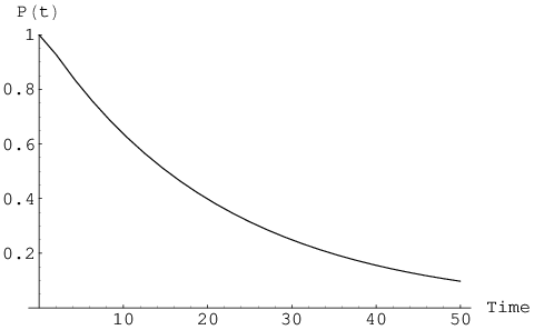
In figure 1 we show the survival probability of the state $|1\rangle$ . As seen in figure 2, the survival probability shows non-exponential decay around $t=0$ (Zeno effect). Figure 3 shows the field generated by the initial condition of excited atom state and no field. We define the field bra $\langle\psi(x)|$ as

	$\displaystyle\langle\psi(x)\|$	$\displaystyle\equiv$	$\displaystyle\int_{-\infty}^{\infty}dk\;\frac{1}{\sqrt{2\omega_{k}}}e^{ikx}\langle k\|$		(19)
		$\displaystyle=$	$\displaystyle\int_{0}^{\infty}d\omega\;\sqrt{\frac{2}{\omega}}\cos(\omega x)\langle\omega\|,$		(19)

The generated field is a superposition of field associated with the Zeno effect, exponential field due to spontaneous emission and dressing cloud around the atom at $x=0$ POP. Note that the field disappears rapidly outside the light cone, defined by $|x|=ct$ with $c=1$ .

Refer to caption — Figure 1: The decay of survival probability $|\langle 1|e^{-iHt}|1\rangle|^{2}$ .

One way to get pure exponential decay is to construct eigenstates with complex eigenvalues. This has been done already, but previous constructions had their own difficulties, for example the exponential growth of the emitted field outside the light cone (exponential catastrophe). In the following sections, we review the approach based on contour deformation.

III Unstable state using contour deformation

In this section we review the construction of unstable state through contour deformation. The construction of complex eigenstate through contour deformation was done by Sudarshan, Chiu, and Gorgini Sudarshan. Later by the perturbation expansion with regularization rules, Petrosky, Prigogine and Tasaki PPT investigated the Friedrichs model and showed that the system can be described as a sum of a discrete complex eigenstate plus continuum states. They showed that their decomposition can be also derived by contour deformation. Let us follow their construction in the Friedrichs model.

In the Friedrichs model, first we note that $\eta^{+}(z)=0$ has a complex root $z_{1}={\tilde{\omega}}_{1}-i\gamma=\omega_{1}+O(\lambda^{2})$ for $0<\omega_{1}\sim O(1)$ . We can consider this as a complex eigenvalue which coincides with the original discrete eigenvalue $\omega_{1}$ in the limit $\lambda\rightarrow 0$ . By contour deformation, we can separate $z_{1}$ pole from $1/\eta^{+}(z)$ in the completeness relation.

	$\displaystyle 1$	$\displaystyle=$	$\displaystyle\int_{0}^{\infty}d\omega\;\|F_{\omega}^{+}\rangle\langle F_{\omega}^{+}\|$		(20)
		$\displaystyle=$	$\displaystyle\int_{\Gamma}d\omega\;\|F_{\omega}^{+}\rangle\langle F_{\omega}^{+}\|+\int_{C}d\omega\;\|F_{\omega}^{+}\rangle\langle F_{\omega}^{+}\|$		(20)

where the contours $\Gamma$ and $C$ are shown in Fig 4.

The pole part of the contour $\int_{C}$ can be written as

\displaystyle\int_{C}d\omega\;|F_{\omega}^{+}\rangle\langle F_{\omega}^{+}|=|\phi_{1}\rangle\langle{\tilde{\phi}}_{1}|

(21)

where

	$\displaystyle\|\phi_{1}\rangle=N_{1}^{1/2}\left(\|1\rangle+\int_{0}^{\infty}d\omega\frac{\lambda v_{\omega}\|\omega\rangle}{z_{1}^{+}-\omega}\right),$		(22)
	$\displaystyle\langle{\tilde{\phi}}_{1}\|=N_{1}^{1/2}\left(\langle 1\|+\int_{0}^{\infty}d\omega\frac{\lambda v_{\omega}\langle\omega\|}{z_{1}^{+}-\omega}\right),$		(23)
	$\displaystyle N_{1}\equiv\left(1+\int_{0}^{\infty}d\omega\frac{\lambda^{2}v_{\omega}^{2}}{(z_{1}^{+}-\omega)^{2}}\right)^{-1}.$		(24)

This complex eigenstate $|\phi_{1}\rangle$ satisfies the eigenvalue equation

\displaystyle H|\phi_{1}\rangle=z_{1}|\phi_{1}\rangle.

(25)

Note that $|\phi_{1}\rangle$ cannot be in the Hilbert space since it has a complex eigenvalue.

It should be noted that when we act a function on $|\phi_{1}\rangle$ the function should not blow up on the deformed contour. We need suitable test functions depending on our choice of contour deformation. Without the test function consideration, unphysical growth (exponential catastrophe) appears. This exponential catastrophe is a main difficulty of accepting this complex eigenstate as a representation of unstable states.

To see this problem let us consider the time evolution of $|\phi_{1}\rangle$ for the atom component and field component. The atom component of $|\phi_{1}\rangle$ is given by

\displaystyle\langle 1|e^{-iHt}|\phi_{1}\rangle=N_{1}^{1/2}e^{-iz_{1}t}.

(26)

Eq. (26) holds for all $t$ . For $t<0$ , the RHS of Eq. (26) grows exponentially. If we had chosen the $-$ branch of the Friedrichs eigenstates as a starting point, then we would have a similar problem: the states would decay for $t<0$ and would grow exponentially for $t>0$ .

This exponential growth also appears in the field component of $|\phi_{1}\rangle$ . The time evolution of this component is becomes

	$\displaystyle\langle\psi(x)\|e^{-iHt}\|\phi_{1}\rangle$	$\displaystyle=$	$\displaystyle e^{-iz_{1}t}\langle\psi(x)\|\phi_{1}\rangle\sim O(e^{-iz_{1}(t-\|x\|)})$		(27)
			for large $\|t-\|x\|\|.$		(27)

The field component shows exponential growth in $x$ . The $|\langle\psi(x)|e^{-iHt}|\phi_{1}\rangle|^{2}$ plot in $x$ space for a fixed time is shown in Fig 5.

We can avoid the exponential growth by choosing suitable test function spaces. One such approach is due to Bohm and Gadella Bohm. They defined complex states (Gamow vectors) through the poles of the S-matrix, and restricted their test function space to Hardy class functions from below. In Appendix A we review their approach and also discuss difficulties in their approach.

In the next section we propose a new way to construct the unstable state for the Friedrichs model. We separate the pole according to the type of test function, and discuss the advantages of our construction over the previous constructions of unstable states.

IV A new unstable state in the Friedrichs model

In this section we propose a new way of defining the unstable state. We want our unstable state to be memoryless and have no unphysical growth. To this end, we construct a complex eigenstate of the time evolution operator $e^{-iHt}$ which gives exponential decay, and a suitable test function space which removes unphysical growth.

IV.1 Complex pole and integration contour

The complex eigenstate is related to the complex pole of Green’s function $[\eta^{+}(z)]^{-1}$ (or the pole of S-matrix $\eta^{-}(\omega)/\eta^{+}(\omega)$ ) that can be calculated by perturbation from the original unperturbed eigenstate. Consider the emission of the field by the excited atom. We focus on the overlap $\langle f|e^{-iHt}|1\rangle$ between the emitted field and a wave packet $\langle f|$ . We restrict our attention to the case in which the wave packet $\langle f|x\rangle$ is square integrable and localized, with compact support in space representation.

From the completeness relation of eigenstates of $H$ , we have

	$\displaystyle\langle f\|e^{-iHt}\|1\rangle$	$\displaystyle=$	$\displaystyle\langle f\|e^{-iHt}\int_{0}^{\infty}d\omega\;\|F_{\omega}^{+}\rangle\langle F_{\omega}^{+}\|1\rangle$		(28)
		$\displaystyle=$	$\displaystyle\int_{0}^{\infty}d\omega e^{-i\omega t}\frac{\eta^{-}(\omega)}{\eta^{+}(\omega)}\langle f\|F_{\omega}^{-}\rangle\langle F_{\omega}^{+}\|1\rangle\$		(29)

In Eq. (28), $1/\eta^{+}(\omega)$ has the pole $z_{1}={\tilde{\omega}}_{1}-i\gamma=\omega_{1}+O(\lambda^{2})$ in the lower half plane. This is the pole we want to extract.

Our task is to take the residue at the pole $z_{1}$ in an integral of the form $\int_{0}^{\infty}d\omega\;h(\omega)$ , where $h(\omega)$ has the pole $z_{1}$ in the lower half of the complex plane. One simple way to do this is making a contour which encloses the pole and using the residue theorem. Suppose that we make a counterclockwise contour $C$ around the pole $z_{1}$ . If $h(\omega)$ is analytic in $C$ , we have

	$\displaystyle\int_{C}d\omega\;h(\omega)=\int_{C}d\omega\;\frac{1}{\omega-z_{1}}h(\omega)(\omega-z_{1})=2\pi ih_{1}(z)$
			(30)

where $h_{1}(\omega)$ is defined as

\displaystyle h_{1}(\omega)\equiv(\omega-z_{1})h(\omega).

(31)

Note that $h_{1}(\omega)$ is analytic function inside $C$ .

The enclosing contour should be chosen according to the test function $\langle f|$ . It would not be a good choice of contour if the test function blows up at the contour. Also, the test function space should be determined by considering underlying physics.

In scattering experiment usually a localized wave packet is prepared. Say $\langle f|x\rangle$ is zero outside the region $-x_{0}<x<x_{0}$ . In our Hamiltonian system, $\langle f|\omega\rangle$ is given by

\displaystyle\langle f|\omega\rangle=\int_{-\infty}^{\infty}dx\;\langle f|x\rangle\langle x|\omega\rangle=\int_{-x_{0}}^{x_{0}}dx\;\langle f|x\rangle\frac{\cos(\omega x)}{\sqrt{\pi}}.

(32)

According to a theorem due to Paley and Wiener Boas, the function $\langle f|\omega\rangle$ is entire function of exponential type $x_{0}$ and belongs to $L^{2}$ on the real axis of $\omega$ (see Appendix B). This theorem shows that even though $\langle f|\omega\rangle$ is $L^{2}$ on the positive real axis, it can be extended to the whole real axis and remain in $L^{2}$ . So, we can use the whole real axis as a part of enclosing contour. We write

\displaystyle\int_{0}^{\infty}=\int_{-\infty}^{\infty}-\int_{-\infty}^{0}

(33)

The last term is a “background” integral, which does not give any pole contribution.

To enclose the pole in the lower half plane, we need another piece of contour besides the real axis. If the function vanishes at the lower infinite semicircle, then the integral over the real axis is the same as the integral over the closed contour consisting of the real axis and the infinite lower semicircle, which encloses the $z_{1}$ pole. For the Cauchy integral

\frac{-1}{2\pi i}\int_{-\infty}^{\infty}d\omega\;\frac{h_{1}(\omega)}{\omega-z_{1}}

with $h_{1}(\omega)$ vanishing on the lower infinite semicircle, we can separate the $z_{1}$ pole residue by subtracting the other pole residues.

\displaystyle\frac{-1}{2\pi i}\int_{-\infty}^{\infty}d\omega\;\frac{h_{1}(\omega)}{\omega-z_{1}}-\sum_{n}{\rm Res}[\frac{h_{1}(\omega)}{\omega-z_{1}}]\bigg|_{p_{n}}=h_{1}(z_{1})

(34)

In Eq. (34), $p_{n}$ are possible poles of $h(\omega)$ other than $z_{1}$ in the lower half plane.

The physical meaning of the test function vanishing at the lower infinite semicircle is causality, as we discuss next.

IV.2 Hardy-class test functions and causality

In Eq. (28) we want to separate the part of the integrand that vanishes at the lower infinite semicircle in $\omega$ plane. This can be done through the decomposition into Hardy-class functions from below and from above, which we define now.

A complex function $G(E)$ on the real line is a Hardy class function from above $H^{2}_{+}$ (below $H^{2}_{-}$ ) if

(1) $G(E)$ is the boundary value of a function $G(\omega)$ of complex variable (complex energy) $\omega=E+i\eta$ that is analytic in the half plane $\eta>0$ ( $\eta<0$ ).

(2)

\int_{-\infty}^{\infty}|G(E+i\eta)|^{2}dE<\mbox{finite}

for all $\eta$ with $0<\eta<\infty$ ( $-\infty<\eta<0$ ).

The function $G(E)$ is called an $H^{2}_{\pm}$ class function. There is an interesting relation between Hardy class functions and $L^{2}$ functions.

Any $L^{2}$ function can be uniquely expressed as the sum of a function in $H^{2}_{-}$ and a function in $H^{2}_{+}$ . If a function $f(\omega)$ is in $L^{2}$ on the real line, we can write

\displaystyle f(\omega)=f^{+}(\omega)+f^{-}(\omega)

(35)

with

	$\displaystyle f^{+}(\omega)\equiv\frac{1}{2\pi i}\int_{-\infty}^{\infty}d\omega^{\prime}\frac{f(\omega^{\prime})}{\omega^{\prime}-\omega-i\epsilon}\in H^{2}_{+},$
	$\displaystyle f^{-}(\omega)\equiv\frac{-1}{2\pi i}\int_{-\infty}^{\infty}d\omega^{\prime}\frac{f(\omega^{\prime})}{\omega^{\prime}-\omega+i\epsilon}\in H^{2}_{-}.$		(36)

We can also write

	$\displaystyle f^{+}(\omega)=\frac{1}{\sqrt{2\pi}}\int_{0}^{\infty}dt\;\hat{f}(t)e^{i\omega t},$
	$\displaystyle f^{-}(\omega)=\frac{1}{\sqrt{2\pi}}\int_{-\infty}^{0}dt\;\hat{f}(t)e^{i\omega t}$		(37)

where

\displaystyle\hat{f}(t)=\frac{1}{\sqrt{2\pi}}\int_{-\infty}^{\infty}d\omega f(\omega)e^{-i\omega t}.

(38)

$f^{\pm}$ has the following properties.

	$\displaystyle\frac{1}{2\pi i}\int_{-\infty}^{\infty}d\omega\frac{f^{+}(\omega)}{\omega-z}=\left\{\begin{array}[]{ll}f^{+}(z)&\mbox{for $Im(z)>0$}\\ 0&\mbox{for $Im(z)<0$}\end{array}\right.$
	$\displaystyle\frac{-1}{2\pi i}\int_{-\infty}^{\infty}d\omega\frac{f^{-}(\omega)}{\omega-z}=\left\{\begin{array}[]{ll}0&\mbox{for $Im(z)>0$}\\ f^{-}(z)&\mbox{for $Im(z)<0$}\end{array}\right.$

The Fourier transform of $f^{\pm}(\omega)$ has the property

\displaystyle\hat{f}^{+}(t)=0\;\;\;\mbox{for $t<0$},\;\;\;\hat{f}^{-}(t)=0\;\;\;\mbox{for $t>0$}

(45)

The most important property for us is that a Hardy-class function from above (below) vanishes at the upper (lower) infinite semicircle in $\omega$ plane.

From Eq. (28) we get

	$\displaystyle\langle f\|e^{-iHt}\|1\rangle$	(46)
$\displaystyle=$	$\displaystyle\int_{0}^{\infty}d\omega\,e^{-i\omega t}\frac{\eta^{-}(\omega)}{\eta^{+}(\omega)}\left[\langle f\|\omega\rangle+\frac{\lambda v_{\omega}}{\eta^{-}(\omega)}\langle f\|1\rangle\right.$	(46)
$\displaystyle+$	$\displaystyle\left.\frac{\lambda v_{\omega}}{\eta^{-}(\omega)}\int_{0}^{\infty}d\omega^{\prime}\frac{\lambda v_{\omega^{\prime}}\langle f\|\omega^{\prime}\rangle}{\omega-\omega^{\prime}-i\epsilon}\right]\frac{\lambda v_{\omega}}{\eta^{-}(\omega)}.$	(47)

For $t\geq 0$ , the second and third terms in the bracket $[\,\,]$ always vanish at the lower infinite semicircle in $\omega$ plane, if they are finite at the real line. The first term vanishes at the lower infinite semicircle if

\displaystyle\left[e^{-i\omega t}\langle f|\omega\rangle\right]^{+}=0

(48)

To see the physical meaning of this condition we write (see Eq. (32))

			$\displaystyle e^{-i\omega t}\langle f\|\omega\rangle=\int_{-\infty}^{\infty}dx\langle f\|x\rangle e^{-i\omega t}\frac{\cos(\omega x)}{\sqrt{\pi}}$		(49)
		$\displaystyle=$	$\displaystyle\frac{1}{2\sqrt{\pi}}\int_{-\infty}^{\infty}dx\langle f\|x\rangle(e^{-i\omega(t-\|x\|)}+e^{-i\omega(t+\|x\|)}).$		(49)

Hence

			$\displaystyle\left[e^{-i\omega t}\langle f\|\omega\rangle\right]^{+}$		(50)
		$\displaystyle=$	$\displaystyle\frac{1}{2\sqrt{\pi}}\int_{0}^{\infty}dx\left(\langle f\|x+t\rangle+\langle f\|-x-t\rangle\right)e^{i\omega x}$		(50)

This vanishes when $t>|x_{0}|$ , the time required for the emitted outgoing wave to have an overlap with the wave packet. This is causality condition follows from the requirement that the integrand in Eq. (46) vanishes at the lower infinite semicircle in order to take the residue at the pole $z_{1}$ . One point to note is that we considered the space and time together when we apply this condition of vanishing at the lower infinite semicircle.

IV.3 Residue at the pole and unstable state

Now we take the residue at the pole $z_{1}$ in Eq. (46). When Eq. (48) is satisfied we get

			$\displaystyle{\rm Res}\left[\langle f\|e^{-iHt}\|1\rangle\right]_{z_{1}}=\langle f\|e^{-iHt}\|\phi_{1}\rangle\langle{\tilde{\phi}}_{1}\|1\rangle$		(51)
		$\displaystyle=$	$\displaystyle e^{-iz_{1}t}\langle f\|\phi_{1}\rangle\langle{\tilde{\phi}}_{1}\|1\rangle\,\,{\rm if\,}\left[e^{-i\omega t}\langle f\|\omega\rangle\right]^{+}=0$		(51)

where $|\phi_{1}\rangle$ is the complex eigenvector of Hamiltonian in Eq. (22) . To generalize this result, we define the space of test functions ${\cal E}_{H}$ as the set of functions $\langle f|e^{-iHt}|\omega\rangle$ with $t\geq 0$ and $\langle f|x\rangle$ being in $L^{2}$ and having compact support. This also implies that $\langle f|\omega\rangle$ is $L^{2}$ and exponential type by Paley and Wiener theorem. Due to the form factor $v_{\omega}$ of our model (see Eq. (2)), $\langle f|F_{\omega}^{\pm}\rangle$ is also exponentially bounded. For these test-functions we introduce a decomposition into a component which vanishes at the lower infinite semicircle in $\omega$ plane and a non-vanishing component.

\displaystyle f(\omega)=f^{v}(\omega)+f^{nv}(\omega)

(52)

Precisely speaking, we denote $f^{nv}(\omega)$ as the part whose maximum modulus grows exponentially as the function approaches the lower infinite semicircle.

Next, we define our custom complex delta function $\delta_{a}(\omega-z_{1})$ as

			$\displaystyle\int_{0}^{\infty}d\omega\;f(\omega)\delta_{a}(\omega-z_{1})$		(53)
		$\displaystyle=$	$\displaystyle\int_{0}^{\infty}d\omega\;(f^{v}(\omega)+f^{nv}(\omega))\delta_{a}(\omega-z_{1})\equiv f^{v}(z_{1}).$		(53)

This delta function is similar to the complex delta functions defined in Nakanishi, except that it takes only the part of test functions which vanishes at the lower infinite semicircle.

If we do not restrict the test functions, we get the complex spectral decomposition

\displaystyle\int_{0}^{\infty}d\omega|F_{\omega}^{+}\rangle\langle F_{\omega}^{+}|=|\phi_{1}\rangle\langle{\tilde{\phi}}_{1}|+\int_{0}^{\infty}d\omega|F_{\omega d}\rangle\langle F_{\omega}^{+}|

(54)

where

\displaystyle|F_{\omega d}^{+}\rangle\equiv|\omega\rangle+\frac{\lambda v_{\omega}}{\eta^{+d}(\omega)}|1\rangle+\frac{\lambda v_{\omega}}{\eta^{+d}(\omega)}\int_{0}^{\infty}d\omega^{\prime}\frac{\lambda v_{\omega^{\prime}}|\omega^{\prime}\rangle}{\omega-\omega^{\prime}+i\epsilon}

with

\displaystyle\frac{1}{\eta^{+d}(\omega)}\equiv\frac{1}{\eta^{+}(\omega)}\frac{z_{1}-\omega}{z_{1}^{+}-\omega}.

(56)

With delta function $\delta_{a}(\omega-z_{1})$ which restricts the test functions to the part which vanishes at the lower infinite semicircle, we devise another expression. Generally it is not easy to define $f(\omega)^{v}$ and $f(\omega)^{nv}$ for function $f(\omega)$ . But for the function $\langle f|\omega\rangle\in\cal E_{H}$ , we can define

	$\displaystyle\langle f\|\omega\rangle^{v}\equiv\langle f\|\omega\rangle^{-},\;\;\langle f\|\omega\rangle^{nv}\equiv\langle f\|\omega\rangle^{+},$		(57)
	$\displaystyle\langle f\|F_{\omega}^{+}\rangle^{v}$		(58)
	$\displaystyle\equiv\langle f\|\omega\rangle^{-}+\frac{\lambda v_{\omega}}{\eta^{+}(\omega)}\langle f\|1\rangle+\frac{\lambda v_{\omega}}{\eta^{+}(\omega)}\int_{0}^{\infty}d\omega^{\prime}\frac{\lambda v_{\omega^{\prime}}\langle f\|\omega^{\prime}\rangle^{-}}{\omega-\omega^{\prime}+i\epsilon}$
	$\displaystyle+\frac{\lambda v_{\omega}}{\eta^{+}(\omega)}\int_{0}^{\infty}d\omega^{\prime}\frac{\lambda v_{\omega^{\prime}}\langle f\|\omega^{\prime}\rangle^{+}}{\omega-\omega^{\prime}-i\epsilon},$
	$\displaystyle\langle f\|F_{\omega}^{+}\rangle^{nv}\equiv\frac{-2\pi i\lambda^{2}v_{\omega}^{2}}{\eta^{+}(\omega)}\langle f\|\omega\rangle^{+},$		(59)
	$\displaystyle\langle f\|F_{\omega}^{-}\rangle^{v}$		(60)
	$\displaystyle\equiv\langle f\|\omega\rangle^{-}+\frac{\lambda v_{\omega}}{\eta^{-}(\omega)}\langle f\|1\rangle+\frac{\lambda v_{\omega}}{\eta^{-}(\omega)}\int_{0}^{\infty}d\omega^{\prime}\frac{\lambda v_{\omega^{\prime}}\langle f\|\omega^{\prime}\rangle}{\omega-\omega^{\prime}-i\epsilon},$
	$\displaystyle\langle f\|F_{\omega}^{-}\rangle^{nv}\equiv\langle f\|\omega\rangle^{+}$		(61)

Because of equations (58)- (61), the definitions of $f^{v}$ and $f^{nv}$ are different from Hardy class functions.

With these definitions we now define the unstable state and its dual as

	$\displaystyle\|\phi_{1a}\rangle\equiv N_{1}^{1/2}\left(\|1\rangle+\int_{0}^{\infty}d\omega\;\frac{\lambda v_{\omega}\|\omega\rangle}{z_{1}^{a}-\omega}\right)$		(62)
	$\displaystyle\langle{\tilde{\phi}}_{1a}\|\equiv N_{1}^{1/2}\left(\langle 1\|+\int_{0}^{\infty}d\omega\;\frac{\lambda v_{\omega}\langle\omega\|}{z_{1}^{a}-\omega}\right).$		(63)

where

\displaystyle\frac{1}{z_{1}^{a}-\omega}\equiv\frac{1}{z_{1}-\omega}-2\pi i\delta_{a}(\omega-z_{1}).

(64)

This gives

	$\displaystyle\langle f\|\phi_{1a}\rangle\equiv N_{1}^{1/2}\bigg(\langle f\|1\rangle$
	$\displaystyle+\int_{0}^{\infty}d\omega\;\frac{\lambda v_{\omega}\langle f\|\omega\rangle^{v}}{z_{1}^{+}-\omega}+\int_{0}^{\infty}d\omega\;\frac{\lambda v_{\omega}\langle f\|\omega\rangle^{nv}}{z_{1}-\omega}\bigg)$		(65)
	$\displaystyle\langle{\tilde{\phi}}_{1a}\|g\rangle\equiv N_{1}^{1/2}\bigg(\langle 1\|g\rangle$
	$\displaystyle+\int_{0}^{\infty}d\omega\;\frac{\lambda v_{\omega}\langle\omega\|g\rangle^{v}}{z_{1}^{+}-\omega}+\int_{0}^{\infty}d\omega\;\frac{\lambda v_{\omega}\langle\omega\|g\rangle^{nv}}{z_{1}-\omega}\bigg).$		(66)

Note that if $\langle f|\omega\rangle^{nv}=0$ then $\langle f|\phi_{1a}\rangle=\langle f|\phi_{1}\rangle$ .

This unstable state $|\phi_{1a}\rangle$ becomes a complex eigenstate of the $e^{-iHt}$ for special kind of test functions. Using (see Appendix C)

\displaystyle\langle F^{-}_{\omega}|\phi_{1a}\rangle=-2\pi iN_{1}^{1/2}\lambda v_{\omega}\delta_{a}(\omega-z_{1})

(67)

and

\displaystyle\eta^{-}(z_{1})=-2\pi i\lambda^{2}v_{z_{1}}^{2},

(68)

we have a complex eigenvalue equation (for $t\geq 0$ )

\displaystyle\langle f|e^{-iHt}|\phi_{1a}\rangle=e^{-iz_{1}t}\langle f|\phi_{1a}\rangle

(69)

if $\langle f|e^{-iHt}|\omega\rangle$ is in $\cal E_{H}$ and vanishes at the lower infinite semicircle, i.e., if $\langle f|$ has compact support in space and $\left(e^{-i\omega t}\langle f|\omega\rangle\right)^{+}=0$ .

When $\left(e^{-i\omega t}\langle f|\omega\rangle\right)^{+}\neq 0$ , we have

	$\displaystyle\langle f\|e^{-iHt}\|\phi_{1a}\rangle$
	$\displaystyle=N_{1}^{1/2}e^{-iz_{1}t}\bigg(\langle f\|1\rangle+\int_{0}^{\infty}d\omega\frac{\lambda v_{\omega}\langle f\|\omega\rangle}{z_{1}^{+}-\omega}$
	$\displaystyle+(-2\pi i\lambda v_{z_{1}})(e^{iz_{1}t}[e^{-i\omega t}\langle f\|\omega\rangle^{+}]^{-}_{z_{1}}-\langle f\|\omega\rangle^{+}_{z_{1}})\bigg).$
			(70)

As we see later in next section the exponentially growing part is removed in Eq. (70).

Eq. (69) is clearly different from the usual eigenvalue equation. We make comments about this equation here. First, this equation is an eigenvalue equation in a restricted test function space. The test function restriction is made according to the physics of the system and causality condition. Second, it is an eigenvalue equation of the time evolution operator $e^{-iHt}$ , rather than $H$ . In following sections we will discuss the space-time behavior of this new unstable state and possible complex spectral representations.

Note that here we have focused on the semi-group that gives decay for $t>0$ . In a similar fashion, we can get results for the other semi-group with decay for $t<0$ starting with the $-$ branch of the Friedrichs eigenstates, and exchanging the roles of functions which vanish at the lower infinite semicircle and functions which vanish at the upper infinite semicircle.

IV.4 Time evolution of unstable state

We act the time evolution operator $e^{-iHt}$ on the state $|\phi_{1a}\rangle$ . The atom component of time evolved ket becomes

	$\displaystyle\langle 1\|e^{-iHt}\|\phi_{1a}\rangle=\langle 1\|e^{-iHt}\int_{0}^{\infty}d\omega\|F^{-}_{\omega}\rangle\langle F^{-}_{\omega}\|\phi_{1a}\rangle$	(71)
$\displaystyle=$	$\displaystyle\langle 1\|\int_{0}^{\infty}d\omega\;e^{-i\omega t}\|F^{-}_{\omega}\rangle(-2\pi iN_{1}^{1/2}\lambda v_{\omega})\delta_{a}(\omega-z_{1})$
$\displaystyle=$	$\displaystyle N_{1}^{1/2}\Theta(t)e^{-iz_{1}t}.$

The atom component of time evolution of $|\phi_{1a}\rangle$ shows exact exponential decay for $t\geq 0$ . This is a semi-group time evolution. Note also the exponential growth for the negative $t$ was removed.

Similarly, the field component of $|\phi_{1a}\rangle$ is (see Appendix D)

	$\displaystyle\langle\psi(x)\|e^{-iHt}\|\phi_{1a}\rangle=\langle\psi(x)\|e^{-iHt}\int_{0}^{\infty}d\omega\|F^{-}_{\omega}\rangle\langle F^{-}_{\omega}\|\phi_{1a}\rangle$
	$\displaystyle=-2\pi i\lambda N_{1}^{1/2}\frac{\pi^{1/2}}{1+z_{1}^{2}/M^{2}}e^{-iz_{1}(t-\|x\|)}\Theta(t-\|x\|)$
	$\displaystyle+2\lambda N_{1}^{1/2}\lambda\frac{z_{1}}{(1+z_{1}^{2}/M^{2})M}e^{-iz_{1}t}e^{-M\|x\|}\Theta(t)$		(72)
	$\displaystyle-2\lambda N_{1}^{1/2}\int_{0}^{\infty}d\omega^{\prime}\frac{\cos(\omega^{\prime}x)}{(1+\omega^{{}^{\prime}2}/M^{2})(z_{1}+\omega^{\prime})}e^{-iz_{1}t}\Theta(t)$

The first term in Eq. (72) comes from the complex pole at $z_{1}$ . This is the travelling field with complex frequency inside the light cone. It corresponds to the decay product. The second term and third term do not travel but decay with time. The second term is due to the non-locality of the interaction, caused by the ultraviolet cutoff in Eq. (2). The third term describes the cloud surrounding the atom POP. It is due to the background integral Bohm2.

None of the terms in Eq. (72) has exponential blowup. The plot of $|\langle\psi(x)|e^{-iHt}|\phi_{1a}\rangle|^{2}$ and $|\langle\psi(x)|e^{-iHt}|1\rangle|^{2}$ in space is shown in Fig 6. For weak coupling the field component of new unstable state is very close to the field component of bare atom decay. The field component of the new unstable state shows a sharp wave front, as the second and third terms in Eq. (A) give negligible contributions. We note that if we had included virtual transitions in the Hamiltonian, the background contribution would also be strictly confined within the light cone Comp.

IV.5 Complex spectral representation of $\exp(-iHt)$

Let us apply the complex delta function $\delta_{a}(\omega-z_{1})$ to the complete set of Friedrichs eigenstates of $H$ .The effect of pole enclosing contour is obtained by multiplying $(-2\pi i)(\omega-z_{1})\delta_{a}(\omega-z_{1})$ to the Friedrichs solution and integrating over $\omega$ . The factor $-2\pi i$ appears since the real axis and lower infinite semicircle clockwisely enclose the lower half plane pole. By this operation we get the $z_{1}$ residue of the part of the test function that vanishes at the lower infinite semicircle.

Consider the inner product $\langle f|e^{-iHt}|g\rangle$ where $\langle f|\omega\rangle$ and $\langle\omega|g\rangle$ are in $\cal E_{H}$ . We have

	$\displaystyle\langle f\|e^{-iHt}\|g\rangle=\int_{0}^{\infty}d\omega\;e^{-i\omega t}\langle f\|F^{+}_{\omega}\rangle\langle F^{+}_{\omega}\|g\rangle$	(73)
$\displaystyle=$	$\displaystyle\int_{0}^{\infty}d\omega\;e^{-i\omega t}\langle f\|F^{+}_{\omega}\rangle\langle F^{+}_{\omega}\|g\rangle(-2\pi i)(\omega-z_{1})\delta_{a}(\omega-z_{1})$
$\displaystyle+$	$\displaystyle\int_{0}^{\infty}d\omega\;e^{-i\omega t}\langle f\|F^{+}_{\omega}\rangle\langle F^{+}_{\omega}\|g\rangle$
$\displaystyle\times$	$\displaystyle(1-(-2\pi i)(\omega-z_{1})\delta_{a}(\omega-z_{1})).$

In Eq. (73), the first term in the right hand side will give the pole separation we wanted. By definition, $\delta_{a}(\omega-z_{1})$ selects the part of $e^{-i\omega t}\langle f|F_{\omega}^{-}\rangle\langle F_{\omega}^{+}|g\rangle$ which vanishes at the lower infinite semicircle. That contains the term $e^{-i\omega t}\langle f|\omega\rangle\langle\omega|g\rangle$ . Generally

\displaystyle[e^{-i\omega t}\langle f|\omega\rangle\langle\omega|g\rangle]^{-}\neq e^{-i\omega t}\langle f|\omega\rangle^{-}\langle\omega|g\rangle^{-},

(74)

so the first term in RHS of Eq. (73) is not factorizable to the left and right complex eigenekts. But there are cases in which the factorization is possible, and we show two simple cases.

One case is when all terms vanish at the lower infinite semicircle. This condition is satisfied when $t\geq 0$ and the terms $[e^{-i\omega t}\langle\omega|g\rangle]$ , $[e^{-i\omega t}\langle f|\omega\rangle]$ , and $[e^{-i\omega t}\langle f|\omega\rangle\langle\omega|g\rangle]$ vanish at the lower infinite semicircle (their $+$ components vanish). The physical meaning of these conditions are the following. Suppose that $\langle f|x\rangle$ has a compact support $[-x_{f},x_{f}]$ in $x$ space. By Eq. (32) and Paley-Wiener theorem, $\langle f|\omega\rangle$ is an $L^{2}$ function of exponential type $x_{f}$ . Similarly for $\langle x|g\rangle$ with a compact support $[-x_{g},x_{g}]$ , $\langle\omega|g\rangle$ is an $L^{2}$ function of exponential type $x_{g}$ . When the functions approach to the lower infinite semicircle, $\langle f|\omega\rangle=O(e^{i\omega x_{f}})$ and $\langle\omega|g\rangle=O(e^{i\omega x_{g}})$ . So $[e^{-i\omega t}\langle f|\omega\rangle]^{+}=0$ implies that for time $t>x_{f}$ all the field component of $\langle f|$ is inside the causal region from the atom. Similarly, $[e^{-i\omega t}\langle\omega|g\rangle]^{+}=0$ means that for $t>x_{g}$ all the field component of $|g\rangle$ is inside the causal region from the atom. The condition $[e^{-i\omega t}\langle f|\omega\rangle\langle\omega|g\rangle]^{+}=0$ means that for time $t>x_{f}+x_{g}$ a photon from $g$ can be scattered through the atom and go to the field in $f$ . This is the causality condition of scattering of the field from the region occupied by $|g\rangle$ to the region occupied by $\langle f|$ .

In this case we get

	$\displaystyle\langle f\|e^{-iHt}\|g\rangle$	$\displaystyle=$	$\displaystyle e^{-iz_{1}t}\langle f\|\phi_{1}\rangle\langle{\tilde{\phi}}_{1}\|g\rangle$		(75)
		$\displaystyle+$	$\displaystyle\int_{0}^{\infty}d\omega\;e^{-i\omega t}\langle f\|F_{\omega d}^{+}\rangle\langle F_{\omega}^{+}\|g\rangle.$		(75)

Another case that we can factorize the pole part in Eq. (73) is when $\langle f|\omega\rangle=0$ or $\langle\omega|g\rangle=0$ . In this case (we consider $\langle\omega|g\rangle=0$ . Similar result can be shown for $\langle f|\omega\rangle=0$ .), we get

	$\displaystyle\langle f\|e^{-iHt}\|g\rangle$
	$\displaystyle=N_{1}^{1/2}e^{-iz_{1}t}\bigg(\langle f\|1\rangle+\int_{0}^{\infty}d\omega\frac{\lambda v_{\omega}}{z_{1}^{+}-\omega}$
	$\displaystyle+(-2\pi i\lambda v_{z_{1}})(e^{iz_{1}t}[e^{-i\omega t}\langle f\|\omega\rangle^{+}]^{-}_{z_{1}}-\langle f\|\omega\rangle^{+}_{z_{1}})\bigg)\langle{\tilde{\phi}}_{1}\|g\rangle$
	$\displaystyle+\int_{0}^{\infty}d\omega\;e^{-i\omega t}\langle f\|F_{\omega a}\rangle\langle F_{\omega}^{+}\|g\rangle$		(76)

like Eq. (70), with

\displaystyle|F_{\omega a}^{+}\rangle=|\omega\rangle+\frac{\lambda v_{\omega}}{\eta^{+a}(\omega)}|1\rangle+\frac{\lambda v_{\omega}}{\eta^{+a}(\omega)}\int_{0}^{\infty}d\omega^{\prime}\frac{\lambda v_{\omega^{\prime}}|\omega^{\prime}\rangle}{\omega-\omega^{\prime}+i\epsilon}

where

\displaystyle\frac{1}{\eta^{+a}(\omega)}\equiv\frac{z_{1}-\omega}{z_{1}^{a}-\omega}.

(78)

Eq. (76) becomes Eq. (75) when

\displaystyle[e^{-i\omega t}\langle f|\omega\rangle]^{-}=e^{-iz_{1}t}\langle f|\omega\rangle^{-}_{z_{1}}.

(79)

As explained above, this is the causality condition between the atom and the field. When Eq. (79) is not satisfied, we have Eq. (76) which does not have an exponentially growing part outside the causal region.

V Concluding remarks

In this article we constructed a complex eigenstate with a suitable test functions which does not give an exponential catastrophe in the Friedrichs model. We extended the energy spectrum to the complex plane and separated the complex pole. To separate the pole, we choose a suitable contour enclosing the pole. We established a class of test-functions (vanishing in the lower energy infinite semicircle) for which this pole separation is physically meaningful, giving a causal description of absorption and emission of decay products.

The complex eigenstate constructed by separating the pole contribution in this way showed unique properties. Its atom component has exact exponential decay for the positive time. Its field component consists of a travelling wave with complex frequency inside the light cone. Thus the exponential catastrophe problem was removed.

This complex eigenstate is an eigenstate of time evolution operator $e^{-iHt}$ . The test function restriction is done by considering both time and space, rather than considering only time independent picture. In this way this complex eigenstate captures essential features of unstable particles in the physically meaningful region.

In our opinion, this work is one nice example of constructing quantum mechanics outside the Hilbert space. The Hilbert space is very useful for describing stationary states. The eigenvalues are real, and the conserved norm represents the probability. But in our Hamiltonian, the atom state decays into the field, and the field is absorbed by the atom state. When we consider only the field space, norm is not conserved since fields are absorbed by the atom states, or the atom emits fields. In this case, we don’t need to stick to the Hilbert space formalism, and distributions and suitable test functions can be used.

In this paper the specification and decomposition of our test function space was done for the Friedrichs model, with the dispersion relation $\omega_{k}=|k|$ . Different test function space should be used when the dispersion relation is different. Moreover, we limited the initial test-functions to functions exponentially bounded at infinity. Inclusion of other functions such as Gaussians requires further consideration. Also, we have limited our discussion to Dirac bras or kets. An extension to density operators in Liouville space involves products of distributions, which will be considered in future works.

Acknowledgements.

The authors thank Dr. T. Petrosky for helpful comments. One of authors thank Asia Pacific Center for Theoretical physics for their hospitality. We acknowledge the Engineering Research Program of the Office of Basic Energy Sciences at the U.S. Department of Energy, Grant No DE-FG03-94ER14465, the Robert A. Welch Foundation Grant F-0365, APCTP center for supporting this work.

Appendix A Gamow vector with Hardy class test functions

In this section we review the Gamow vector formalism introduced by Bohm and Gadella, and apply their formalism to the Friedrichs model. We show that the Gamow vector obtained also has difficulties to represent the decaying state. The original derivation of Gamow vectors presented in this section is found in Bohm’s book Bohm2.

In Ref. Bohm2, Gamow vectors are derived by considering S-matrix elements for the scattering of a pure state $\phi^{in}$ into a pure physical state $\psi^{out}$ . $\phi^{in}$ is a controlled free state and determined by the preparation apparatus. $\psi^{out}$ is a free state controlled by the registration apparatus.

When the Hamiltonian can be written as $H=H_{0}+V$ , where $H_{0}$ is the free Hamiltonian and $V$ is the interaction, the exact states $\phi^{+}(t)$ and $\psi^{-}(t)$ are written as

	$\displaystyle\phi^{+}(t)=\phi^{in}(t)+\int_{-\infty}^{\infty}dt^{\prime}\;G^{+}(t-t^{\prime})V\phi^{in}(t^{\prime}),$		(80)
	$\displaystyle\psi^{-}(t)=\psi^{out}(t)+\int_{-\infty}^{\infty}dt^{\prime}\;G^{-}(t-t^{\prime})V\psi^{out}(t^{\prime}).$		(81)

In Eq. (81), the Green’s function $G^{\pm}$ is given by

	$\displaystyle G^{+}(t)=\left\{\begin{array}[]{ll}0\;\;\;\mbox{if $t<0$,}\\ -ie^{-iHt}\;\;\;\mbox{if $t>0$,}\end{array}\right.$
	$\displaystyle G^{-}(t)=\left\{\begin{array}[]{ll}ie^{-iHt}\;\;\;\mbox{if $t<0$,}\\ 0\;\;\;\mbox{if $t>0$.}\end{array}\right.$

Defining the Møller wave operators as

\displaystyle\Omega^{\pm}\equiv I+\int_{-\infty}^{\infty}dt^{\prime}\;G^{\pm}(t-t^{\prime})Ve^{-iH_{0}(t^{\prime}-t)},

(88)

Eq. (80) and Eq. (81) can be written as

\displaystyle\phi^{+}(t)=\Omega^{+}\phi^{in}(t),\;\;\;\;\psi^{-}(t)=\Omega^{-}\psi^{out}(t)

(89)

and the scattering operator $S$ is defined as

\displaystyle S\equiv\Omega^{-\dagger}\Omega^{+}.

(90)

The S-matrix element for $\phi^{in}$ and $\psi^{out}$ becomes

			$\displaystyle(\psi^{out}(t),S\phi^{in}(t))=(\Omega^{-}\psi^{out}(t),\Omega^{+}\phi^{in}(t))$		(91)
		$\displaystyle=$	$\displaystyle(\psi^{-}(t),\phi^{+}(t))=(\psi^{-},\phi^{+})$		(91)

We can calculate Eq. (91) using the eigenvectors of the total Hamiltonian $H$ . If we write the eigenvectors of the free Hamiltonian $H_{0}$ as $|E\rangle$ , the eigenvectors of the total Hamiltonian $H$ can be obtained using the Møller wave operators

	$\displaystyle\|E^{\pm}\rangle=\Omega^{\pm}\|E\rangle,$		(92)
	$\displaystyle H_{0}\|E\rangle=E\|E\rangle,\;\;\;H\|E^{\pm}\rangle=E\|E^{\pm}\rangle.$		(93)

The eigenkets $|E^{+}\rangle$ and $|E^{-}\rangle$ are related by

\displaystyle|E^{+}\rangle=|E^{-}\rangle S(E).

(94)

Using the eigenvectors of total Hamiltonian, Eq. (91) can be written as

\displaystyle(\psi^{-},\phi^{+})=\int_{0}^{\infty}dE\;\langle\psi^{-}|E^{-}\rangle S(E)\langle E^{+}|\phi^{+}\rangle

(95)

We assume the S-matrix has a single complex pole $Z_{R}$ ,

\displaystyle S(E)=\frac{s_{-1}}{E-Z_{R}}+s_{0}+s_{1}(E-Z_{R})+...

(96)

To introduce the Gamow vector associated with this pole, Bohm and Gadella defined a test function space $\Phi_{-}$ in which functions are Hardy class functions from below and, in addition, are analytic functions that vanish faster than any inverse polynomial at the lower infinite semicircle. It is assumed that $\langle\phi^{-}|E^{-}\rangle$ and $\langle E^{+}|\phi^{+}\rangle$ both belong to $\Phi_{-}$ .

With these properties in mind, we continue our discussion about the Gamow vector. When $\langle\psi^{-}|E^{-}\rangle$ and $\langle E^{+}|\phi^{+}\rangle$ both belong to $H^{2}_{-}$ , we have

			$\displaystyle(\psi^{-},\phi^{+})=\int_{-\infty}^{0}dE\langle\psi^{-}\|E^{-}\rangle S(E)\langle E^{+}\|\phi^{+}\rangle$		(97)
		$\displaystyle+$	$\displaystyle\int_{-\infty}^{\infty}\langle\psi^{-}\|E^{-}\rangle\frac{s_{-1}}{E-Z_{R}}\langle E^{+}\|\phi^{+}\rangle.$		(97)

Here $s_{-1}$ is the residue of $S(E)$ at the complex pole $Z_{R}$ . Using Eq. (IV.2), we can write

			$\displaystyle(\psi^{-},\phi^{+})=\int_{-\infty}^{0}dE\langle\psi^{-}\|E^{-}\rangle S(E)\langle E^{+}\|\phi^{+}\rangle$		(98)
		$\displaystyle+$	$\displaystyle(-2\pi is_{-1})\langle\psi^{-}\|Z_{R}^{-}\rangle\langle Z_{R}^{+}\|\phi^{+}\rangle.$		(98)

Thus omitting the arbitrary vector $\psi^{-}$ in $H^{2}_{-}$ ,

			$\displaystyle\|\phi^{+}\rangle=\int_{0}^{-\infty}dE\|E^{+}\rangle\langle E^{+}\|\phi^{+}\rangle$		(99)
		$\displaystyle+$	$\displaystyle\|Z_{R}^{-}\rangle(-2\pi is_{-1})\langle Z_{R}^{+}\|\phi^{+}\rangle.$		(99)

where the complex eigenvector $|Z_{R}^{-}\rangle$ is given by

\displaystyle|Z_{R}^{-}\rangle=-\frac{1}{2\pi i}\int_{-\infty}^{\infty}dE|E^{-}\rangle\frac{1}{E-Z_{R}},

(100)

which is a functional over $H^{2}_{+}$ only.

If $\langle\psi^{-}|E^{-}\rangle$ belongs to $H^{2}_{-}$ , then the time-evolved state $\langle\psi^{-}|e^{-iHt}|E^{-}\rangle$ becomes also a Hardy class function from below if $t\geq 0$ . Using Eq. (IV.2), we obtain

	$\displaystyle\langle e^{iHt}\psi^{-}\|Z_{R}^{-}\rangle=e^{-iZ_{R}t}\langle\psi^{-}\|Z_{R}^{-}\rangle$
	for $t\geq 0$ and every $\langle\psi^{-}\|E^{-}\rangle$ in $H^{2}_{-}$		(101)

This Gamow vector does show exponential decay and semigroup time evolution for $t\geq 0$ . To see if this definition is suitable for the representation of unstable states, we should also check how the field component of this Gamow vector behaves. We apply the above Gamow vector formalism to the Friedrichs model, and see how its field component is represented in position space.

In the Friedrichs model, the exact eigenvectors $|E^{\pm}\rangle$ are explicitly written as $|F_{\omega}^{\pm}\rangle$ . From the relation

\displaystyle\eta^{+}(\omega)-\eta^{-}(\omega)=2\pi i\lambda^{2}v_{\omega}^{2},

(102)

we can show that

\displaystyle|F^{+}_{\omega}\rangle=\frac{\eta^{-}(\omega)}{\eta^{+}(\omega)}|F^{-}_{\omega}\rangle

(103)

and the scattering matrix $S(\omega)$ is

\displaystyle S(\omega)=\frac{\eta^{-}(\omega)}{\eta^{+}(\omega)}.

(104)

The pole of $S(\omega)$ is at $z_{1}$ , which satisfies $\eta^{+}(z_{1})=0$ . According to the above formalism, the Gamow vector in the Friedrichs model is

\displaystyle|z_{1}^{-}\rangle=-\frac{1}{2\pi i}\int_{-\infty}^{\infty}d\omega\;|F^{-}_{\omega}\rangle\frac{1}{\omega-z_{1}}.

(105)

Let us calculate the field component for this Gamow vector. From Eqs. (19) and (105),

			$\displaystyle\langle\psi(x)\|F_{\omega}^{-}\rangle=\sqrt{\frac{2}{\omega}}\cos(\omega x)$		(106)
		$\displaystyle+$	$\displaystyle\frac{\lambda v_{\omega}}{\eta^{-}(\omega)}\int_{0}^{\infty}d\omega^{\prime}\sqrt{\frac{2}{\omega^{\prime}}}\frac{\lambda v_{\omega^{\prime}}}{\omega-\omega^{\prime}-i\epsilon}\cos(\omega^{\prime}x).$		(106)

In Eq. (106), we separate the component which is in $\Phi_{-}$ . Using Eq. (36) on the second Riemann sheet to separate this component, we get

			$\displaystyle(\langle\psi(x)\|F_{\omega_{II}}^{-}\rangle)_{\Phi_{-}}=2\pi i\frac{\lambda^{2}}{\eta^{-}(\omega)}\sqrt{\frac{\omega}{2}}e^{-i\omega\|x\|}$		(107)
		$\displaystyle\times$	$\displaystyle\left(\frac{1}{4}\frac{1}{(1-i\omega/M)^{2}}+\frac{1}{8}\frac{1}{(1-i\omega/M)}\right)$		(107)

Substituting $\omega=z_{1}$ we obtain the Gamow vector field component

			$\displaystyle\langle\psi(x)\|z_{1}^{-}\rangle=2\pi i\frac{\lambda^{2}}{\eta^{-}(z_{1})}\sqrt{\frac{z_{1}}{2}}e^{-iz_{1}\|x\|}$		(108)
		$\displaystyle\times$	$\displaystyle\left(\frac{1}{4}\frac{1}{(1-iz_{1}/M)^{2}}+\frac{1}{8}\frac{1}{(1-iz_{1}/M)}\right)$		(108)

This shows exponentially decaying behavior for $x$ . If we apply $e^{iHt}\psi(x)$ to the Gamow vector, we get

	$\displaystyle\langle e^{iHt}\psi(x)\|z_{1}\rangle=e^{-iz_{1}t}\langle\psi^{-}(x)\|z_{1}\rangle$	(109)
$\displaystyle=$	$\displaystyle 2\pi i\frac{\lambda^{2}}{\eta^{-}(z_{1})}\sqrt{\frac{z_{1}}{2}}\left(\frac{1}{4}\frac{1}{(1-iz_{1}/M)^{2}}+\frac{1}{8}\frac{1}{(1-iz_{1}/M)}\right)$
$\displaystyle\times$	$\displaystyle e^{-iz_{1}(t+\|x\|)}\mbox{for $t\geq 0$}$

Since we restricted the test function space to the Hardy class functions from below as well as analytic functions that vanish faster than any inverse polynomials at the lower infinite semicircle (the space $\Phi_{-}$ ), the field component of this Gamow vector only gives the tail part of the exponential field $e^{-iz_{1}(t+|x|)}$ , which does not show any wavefront (see figure 7). Actually, the dominant part of the field emitted from the decaying atom has the travelling wave with wavefront at the light cone, proportional to $e^{-iz_{1}(t-|x|)}\theta(t-|x|)$ . The emited field term $e^{-iz_{1}(t-|x|)}\theta(t-|x|)$ originates from the $e^{i\omega|x|}$ term of $\langle\psi(x)|F_{\omega}^{-}\rangle$ , which is outside the space $\Phi_{-}$ .

From the above example, we see that the emitted field is not fully represented by the Gamow vector $|z_{1}\rangle$ with the test function $\langle\psi^{-}|E^{-}\rangle\in\Phi_{-}$ . We need another method to separate the complex pole from the Hamiltonian so that the separated pole term properly represents the decaying atom as well as the emitted field.

Appendix B Paley-Wiener theorem

An entire function is one which is regular for all finite complex arguments. For the regular function $f(z)$ in $|z|<|R|$ , we denote $M(r)$ as the maximum modulus of $f(z)$ for $|z|=r<R$ . For entire functions we take $R\to\infty$ . The entire function $f(z)$ is called of positive order $\rho$ and of type $\tau$ if

\displaystyle\lim_{r\rightarrow\infty}\sup r^{-\rho}\log M(r)=\tau.\;\;\;(0\leq\tau\leq\infty)

(110)

A function of order 1 and type $\tau$ ( $\tau<\infty$ ) is called a function of exponential type.

The theorem by Paley and Wiener states the following.

Theorem by Paley and Wiener.

An entire function $f(z)$ is of exponential type $x_{0}$ and belongs to $L^{2}$ on the real axis if and only if

\displaystyle f(z)=\int_{-x_{0}}^{x_{0}}e^{izx}\phi(x)\;dx,

(111)

where

\displaystyle\phi(x)\in L^{2}(-\infty,\infty).

(112)

Also, if $\phi(x)$ does not vanish almost everywhere in any neighborhood of $x_{0}$ (or $-x_{0}$ ) then $f(z)$ is order 1 and type $x_{0}$ .

Appendix C derivation of Eq. (67)

We have

	$\displaystyle\langle F^{-}_{\omega}\|\phi_{1a}\rangle$
	$\displaystyle=\bigg(\langle\omega\|+\frac{\lambda v_{\omega}}{\eta^{+}(\omega)}\langle 1\|+\frac{\lambda v_{\omega}}{\eta^{+}(\omega)}\int_{0}^{\infty}d\omega^{\prime}\frac{\lambda v_{\omega^{\prime}}\langle\omega^{\prime}\|}{\omega-\omega^{\prime}+i\epsilon}\bigg)N_{1}^{1/2}\bigg(\|1\rangle+\int_{0}^{\infty}d\omega\frac{\lambda v_{\omega}}{z_{1}^{a}-\omega}\|\omega\rangle\bigg)$
	$\displaystyle=N_{1}^{1/2}\bigg(\frac{\lambda v_{\omega}}{z_{1}^{a}-\omega}+\frac{\lambda v_{\omega}}{\eta^{+}(\omega)}+\frac{\lambda v_{\omega}}{\eta^{+}(\omega)}\int_{0}^{\infty}d\omega^{\prime}\frac{\lambda^{2}v_{\omega^{\prime}}^{2}}{(\omega-\omega^{\prime}+i\epsilon)(z_{1}^{a}-\omega^{\prime})}\bigg)$
	$\displaystyle=N_{1}^{1/2}\bigg(\frac{\lambda v_{\omega}}{z_{1}^{a}-\omega}+\frac{\lambda v_{\omega}}{\eta^{+}(\omega)}+\frac{\lambda v_{\omega}}{\eta^{+}(\omega)}\frac{1}{z_{1}-\omega}\bigg\{\int_{0}^{\infty}d\omega^{\prime}\frac{\lambda^{2}v_{\omega^{\prime}}^{2}}{\omega-\omega^{\prime}+i\epsilon}-\int_{0}^{\infty}d\omega^{\prime}\frac{\lambda^{2}v_{\omega^{\prime}}^{2}}{z_{1}^{+}-\omega^{\prime}}\bigg\}\bigg)$
	$\displaystyle=N_{1}^{1/2}\bigg(\frac{\lambda v_{\omega}}{z_{1}^{a}-\omega}+\frac{\lambda v_{\omega}}{\eta^{+}(\omega)}+\frac{\lambda v_{\omega}}{\eta^{+}(\omega)}\frac{1}{z_{1}-\omega}\bigg\{-\eta^{+}(\omega)+\omega-\omega_{1}-z_{1}+\omega_{1}\bigg\}\bigg)$
	$\displaystyle=N_{1}^{1/2}\lambda v_{\omega}\bigg(\frac{1}{z_{1}^{a}-\omega}-\frac{1}{z_{1}-\omega}\bigg)=N_{1}^{1/2}\lambda v_{\omega}(-2\pi i)\delta_{a}(\omega-z_{1}).$		(113)

Appendix D derivation of Eq. (72)

We calculate the field component of $|\phi_{1a}\rangle$ .

	$\displaystyle\langle\psi(x)\|e^{-iHt}\|\phi_{1a}\rangle=\frac{1}{\sqrt{\pi}}\int_{0}^{\infty}d\omega^{\prime}\frac{\cos(\omega^{\prime}x)}{\sqrt{\omega^{\prime}}}\langle\omega^{\prime}\|e^{-iHt}\int_{0}^{\infty}d\omega\|F^{-}_{\omega}\rangle\langle F_{\omega}^{-}\|\phi_{1a}\rangle$
	$\displaystyle=\sqrt{2}\int_{0}^{\infty}d\omega e^{-i\omega t}\bigg[\frac{\cos(\omega x)}{\sqrt{\omega}}+\frac{\lambda v_{\omega}}{\eta^{-}(\omega)}\int_{0}^{\infty}d\omega^{\prime}\frac{\lambda v_{\omega^{\prime}}\cos(\omega^{\prime}x)}{\sqrt{\omega^{\prime}}(\omega-\omega^{\prime}-i\epsilon)}\bigg)]$
	$\displaystyle\times(-2\pi i)N_{1}^{1/2}\lambda v_{\omega}\delta_{a}(\omega-z_{1})$
	$\displaystyle=-2\pi iN_{1}^{1/2}\int_{0}^{\infty}d\omega\bigg[\frac{2\lambda e^{-i\omega t}\cos(\omega x)}{1+\omega^{2}/M^{2}}+e^{-i\omega t}\frac{\lambda^{2}v_{\omega}^{2}}{\eta^{-}(\omega)}\int_{0}^{\infty}d\omega^{\prime}\frac{2\lambda\cos(\omega^{\prime}x)}{(1+\omega^{2}/M^{2})(\omega-\omega^{\prime}-i\epsilon)}\bigg]$
	$\displaystyle\times\delta_{a}(\omega-z_{1}).$		(114)

Although $\langle\psi(x)|\omega\rangle$ has $1/\sqrt{\omega}$ singularity, combined with $v_{\omega}$ the test function for $\delta_{a}(\omega-z_{1})$ in Eq. (114) becomes $L^{2}$ and analytic on the real line, grows at most exponentially at complex infinity with poles due to the form factor. Inside the square bracket of last term in Eq. (114), the separation of the part which vanishes at the lower infinite semicircle and non-vanishing part is clear due to the exponential functions. The vanishing part inside the square bracket in Eq. (114) is

\displaystyle\frac{\lambda e^{-i\omega(t-|x|)}}{2(1+\omega^{2}/M^{2})}\Theta(t-|x|)+e^{-i\omega t}\Theta(t)\frac{\lambda^{2}v_{\omega}^{2}}{\eta^{-}(\omega)}\int_{0}^{\infty}d\omega^{\prime}\frac{\lambda\cos(\omega^{\prime}x)}{(1+\omega^{2}/M^{2})(\omega-\omega^{\prime}-i\epsilon)}.

(115)

Applying $\delta_{a}(\omega-z_{1})$ to the above and rearranging terms, we get Eq. (72).

References

(1) G. Gamow, Z. Phys. 51, 204 (1928).
(2) N. Nakanishi, Prog. Theor. Phys. 19, 607 (1958).
(3) T. D. Lee, Phys. Rev. 95, 1329 (1954).
(4) E.C.G. Sudarshan, C. B. Chiu and V. Gorini, Phys. Rev. D 18, 2914 (1978).
(5) A. Böhm and M. Gadella, Dirac Kets, Gamow Vectors and Gelfand Triplets, (Springer Lecture Notes on Physics, Vol. 348, Springer, New York, 1989).
(6) I. Antoniou, Z. Zuchanecki and S. Tasaki, in Operator Theory and Dynamical Systems edited by I. Antoniou and G. Lummer (Chapman and Hall, London, 1999) p. 130.
(7) T. Petrosky, I. Prigogine and S. Tasaki, Physica A 173, 175 (1991).
(8) G. Ordonez, T. Petrosky and I. Prigogine, Phys. Rev. A 63, 052106 (2001).
(9) G. García-Caldéron, in Symmetries of Physics, edited by A. Frank and K. B. Wolf (Springer-Verlag, New York, 1992), p. 252.
(10) H. M. Nussenzveig, in Symmetries of Physics, edited by A. Frank and K. B. Wolf (Springer-Verlag, New York, 1992), p. 295.
(11) U. Fano, Nuovo Cimento, 12, 156 (1935).
(12) K. Friedrichs, Commun. Pure Appl. Math. 1, 361 (1948).
(13) C. Cohen-Tannouji, J. Dupont-Roc and G. Grynberg, Atom-photon interactions. Basic processes and applications (Wiley, New York, 1992).
(14) I. Prigogine, From being to becoming (Freeman, New York, 1980).
(15) T. Petrosky, G. Ordonez and I. Prigogine, Phys. Rev. A 64, 062101 (2001).
(16) A. Bohm, Quantum Mechanics 3rd ed. (Springer-Verlag, New York, 1993).
(17) R.P. Boas, Entire functions (Academic Press, New york, 1954).
(18) K. Hoffman, Banach spaces of Analytic functions (Dover Publications, Inc. , New York, 1962).
(19) C. Compgano, G. M. Palma, R. Passante and F. Persico, J. Phys. B 28, 1105 (1995).

	$\displaystyle\langle f\|\omega\rangle^{v}\equiv\langle f\|\omega\rangle^{-},\;\;\langle f\|\omega\rangle^{nv}\equiv\langle f\|\omega\rangle^{+},$		(57)
	$\displaystyle\langle f\|F_{\omega}^{+}\rangle^{v}$		(58)
	$\displaystyle\equiv\langle f\|\omega\rangle^{-}+\frac{\lambda v_{\omega}}{\eta^{+}(\omega)}\langle f\|1\rangle+\frac{\lambda v_{\omega}}{\eta^{+}(\omega)}\int_{0}^{\infty}d\omega^{\prime}\frac{\lambda v_{\omega^{\prime}}\langle f\|\omega^{\prime}\rangle^{-}}{\omega-\omega^{\prime}+i\epsilon}$
	$\displaystyle+\frac{\lambda v_{\omega}}{\eta^{+}(\omega)}\int_{0}^{\infty}d\omega^{\prime}\frac{\lambda v_{\omega^{\prime}}\langle f\|\omega^{\prime}\rangle^{+}}{\omega-\omega^{\prime}-i\epsilon},$
	$\displaystyle\langle f\|F_{\omega}^{+}\rangle^{nv}\equiv\frac{-2\pi i\lambda^{2}v_{\omega}^{2}}{\eta^{+}(\omega)}\langle f\|\omega\rangle^{+},$		(59)
	$\displaystyle\langle f\|F_{\omega}^{-}\rangle^{v}$		(60)
	$\displaystyle\equiv\langle f\|\omega\rangle^{-}+\frac{\lambda v_{\omega}}{\eta^{-}(\omega)}\langle f\|1\rangle+\frac{\lambda v_{\omega}}{\eta^{-}(\omega)}\int_{0}^{\infty}d\omega^{\prime}\frac{\lambda v_{\omega^{\prime}}\langle f\|\omega^{\prime}\rangle}{\omega-\omega^{\prime}-i\epsilon},$
	$\displaystyle\langle f\|F_{\omega}^{-}\rangle^{nv}\equiv\langle f\|\omega\rangle^{+}$		(61)

	$\displaystyle\langle f\|\phi_{1a}\rangle\equiv N_{1}^{1/2}\bigg(\langle f\|1\rangle$
	$\displaystyle+\int_{0}^{\infty}d\omega\;\frac{\lambda v_{\omega}\langle f\|\omega\rangle^{v}}{z_{1}^{+}-\omega}+\int_{0}^{\infty}d\omega\;\frac{\lambda v_{\omega}\langle f\|\omega\rangle^{nv}}{z_{1}-\omega}\bigg)$		(65)
	$\displaystyle\langle{\tilde{\phi}}_{1a}\|g\rangle\equiv N_{1}^{1/2}\bigg(\langle 1\|g\rangle$
	$\displaystyle+\int_{0}^{\infty}d\omega\;\frac{\lambda v_{\omega}\langle\omega\|g\rangle^{v}}{z_{1}^{+}-\omega}+\int_{0}^{\infty}d\omega\;\frac{\lambda v_{\omega}\langle\omega\|g\rangle^{nv}}{z_{1}-\omega}\bigg).$		(66)

	$\displaystyle\langle f\|e^{-iHt}\|\phi_{1a}\rangle$
	$\displaystyle=N_{1}^{1/2}e^{-iz_{1}t}\bigg(\langle f\|1\rangle+\int_{0}^{\infty}d\omega\frac{\lambda v_{\omega}\langle f\|\omega\rangle}{z_{1}^{+}-\omega}$
	$\displaystyle+(-2\pi i\lambda v_{z_{1}})(e^{iz_{1}t}[e^{-i\omega t}\langle f\|\omega\rangle^{+}]^{-}_{z_{1}}-\langle f\|\omega\rangle^{+}_{z_{1}})\bigg).$
			(70)

	$\displaystyle\langle\psi(x)\|e^{-iHt}\|\phi_{1a}\rangle=\langle\psi(x)\|e^{-iHt}\int_{0}^{\infty}d\omega\|F^{-}_{\omega}\rangle\langle F^{-}_{\omega}\|\phi_{1a}\rangle$
	$\displaystyle=-2\pi i\lambda N_{1}^{1/2}\frac{\pi^{1/2}}{1+z_{1}^{2}/M^{2}}e^{-iz_{1}(t-\|x\|)}\Theta(t-\|x\|)$
	$\displaystyle+2\lambda N_{1}^{1/2}\lambda\frac{z_{1}}{(1+z_{1}^{2}/M^{2})M}e^{-iz_{1}t}e^{-M\|x\|}\Theta(t)$		(72)
	$\displaystyle-2\lambda N_{1}^{1/2}\int_{0}^{\infty}d\omega^{\prime}\frac{\cos(\omega^{\prime}x)}{(1+\omega^{{}^{\prime}2}/M^{2})(z_{1}+\omega^{\prime})}e^{-iz_{1}t}\Theta(t)$

	$\displaystyle\langle f\|e^{-iHt}\|g\rangle$
	$\displaystyle=N_{1}^{1/2}e^{-iz_{1}t}\bigg(\langle f\|1\rangle+\int_{0}^{\infty}d\omega\frac{\lambda v_{\omega}}{z_{1}^{+}-\omega}$
	$\displaystyle+(-2\pi i\lambda v_{z_{1}})(e^{iz_{1}t}[e^{-i\omega t}\langle f\|\omega\rangle^{+}]^{-}_{z_{1}}-\langle f\|\omega\rangle^{+}_{z_{1}})\bigg)\langle{\tilde{\phi}}_{1}\|g\rangle$
	$\displaystyle+\int_{0}^{\infty}d\omega\;e^{-i\omega t}\langle f\|F_{\omega a}\rangle\langle F_{\omega}^{+}\|g\rangle$		(76)

A new way of defining unstable states

Abstract

pacs

I Introduction

II Model

III Unstable state using contour deformation

IV A new unstable state in the Friedrichs model

IV.1 Complex pole and integration contour

IV.2 Hardy-class test functions and causality

IV.3 Residue at the pole and unstable state

IV.4 Time evolution of unstable state

IV.5 Complex spectral representation of exp⁡(−i​H​t)\exp(-iHt)

V Concluding remarks

Acknowledgements.

Appendix A Gamow vector with Hardy class test functions

Appendix B Paley-Wiener theorem

Theorem by Paley and Wiener.

Appendix C derivation of Eq. (67)

Appendix D derivation of Eq. (72)

References

IV.5 Complex spectral representation of $\exp(-iHt)$