On image reconstruction with the two-dimensional interpolating resistive readout structure of the Virtual-Pixel detector Thanks: Work supported by the European Community (contract no. ERBFMGECT980104).
Abstract
The two-dimensional interpolating readout concept of the Virtual-Pixel detector (ViP detector) goes along with an enormous reduction of electronic channels compared to pure pixel devices. However, the special concept of the readout structure demands for adequate position reconstruction methods. Theoretical considerations reflecting the choice and the combination of linear algorithms with emphasis on correct position reconstruction and spatial resolution are presented. A subsequent two-dimensional coordinate transformation further improves the image response of the system. Measured images show how far the theoretical predictions of the simulations can be verified and to what extent they can be used to improve the position reconstruction.
PACS: 29.40.Gx, 02.60.Cb
Keywords:
Two-dimensional interpolating resistive readout structure; Position reconstruction; Algorithms; Spatial resolution; Population density, , , , , ,
1 Introduction
In general, position sensitive pixel detectors feature the advantages of parallel and asynchronous readout which means i.e. a proportional increase of the maximum incoming rate with the sensitive detection area. However, these pure pixel devices suffer from the enormous number of electronic channels leading either to high costs and effort or essential size limitation of the sensitive area. In contrast to that, interpolating readout concepts which can cover large areas with a position resolution comparable to pure pixel devices can also be carried out with parallel and asynchronous readout. They combine the advantages of pixel detectors with a reduction of electronics and costs at the same time. For example the interpolating readout can be realised by strips or pads [1, 2, 3, 4]. We have developed a truly two-dimensional interpolating readout concept based on resistive charge division [5]. Since this concept requires to count single photons the signal of each event has to be amplified, e.g. by gas amplification. For that purpose e.g. micro pattern devices like GEM11 1 GEM = gas electron multiplier [6], micromegas22 2 micromegas = micro mesh gaseous structure [7] and CAT33 3 CAT = compteur à trous [8] can be applied. We have combined the readout structure with (optimised) MicroCAT gas gain structures [9, 10] and a triple-GEM configuration [11]. In combination with the triple-GEM configuration this readout concept has already proven its possible application in biological and chemical diffraction measurements [12]. In principle this resistive interpolating readout structure can also be applied with vacuum devices like micro channel plates.
Beside the advantages of a good time resolution [13] and high rate capability this two-dimensional interpolation concept demands on the other hand for a sophisticated choice of position reconstruction algorithms and correction functions.
2 Detector setup and working principle
Primary charge generated in the gas conversion region by incoming photons (typical energy range: ) via photoelectric effect is led by an homogeneous electric drift field towards the gas gain region where it is multiplied in an avalanche process. This charge cluster (a so called event) hits the readout plane, designed as a two-dimensional resistive structure, where the sensitive area is subdivided into square, sized cells (Fig. 1).

Each cell is provided with two different surface resistivities in order to obtain both an almost linear charge division behaviour in both coordinates and a good electrical shielding to avoid too large charge distributions over several cells. The high resistivity centres of the cells are surrounded by low resistivity narrow border strips (s. detail in Fig. 1). This leads to an almost perpendicular projection of the charges in - and -direction onto the low resistivity strips. The surface resistances of the high resistivity cell centres and the low resistivity strips are typically – and –, respectively. Each cell is read out at its four corners by low input impedance readout nodes. The charges collected at the particular nodes are used to determine the event position within the cell by means of a suitable algorithm. All 64 readout nodes are equipped with charge sensitive amplifiers and 12-bit FADCs which are linked to a dedicated DAQ system which transfers the preprocessed data for visualisation to a PC [14].
3 The choice of reconstruction algorithms
The first subsection describes the simulation tool which provides the charge distribution within the readout structure. These theoretical data will be used in the following to study the partly unfavourable behaviour of different linear algorithms concerning position reconstruction and spatial resolution. Afterwards, the treated algorithms are combined to one more complex algorithm which unifies the advantages of the individual algorithms.
A remark concerning the notation: The expressions for the derivatives and are used synonymous.
3.1 The diffusion simulation model
Due to the surface resistances and the underlying distributed capacitance the readout structure behaves like an integrating -element resulting in a temporal broadening of the input signal. The simulation of this dynamic charge diffusion process on the readout structure has been realised by means of a numerical computation programme, taking -cells into account in order to include charge flow into adjacent cells (boundary effects). A very detailed derivation of the diffusion model and its numerical solution can be found in Ref. [15]. In the diffusion model a space and time dependent driving current can be impinged at every grid point. In the simulation, presented here, we assumed a typical two-dimensional gaussian-like transverse extension of the charge cloud of (mainly caused by the transverse diffusion of the primary electrons in the conversion gap).
The -cell model provides grid points which correspond to a homogeneous grid point spacing of . The low resistivity border strips have a width of , hence they are represented by one single line of grid points. If not stated differently the readout nodes are represented by one grid point which corresponds to . Since the readout nodes can be well approximated as ideal drains [15] the potential at the nodes is equal to zero at all times.
This time-depending diffusion simulation is able to provide the currents and the charges at every particular node for all times . These simulated charges can now be used to reconstruct the event position by means of a suitable algorithm. Depending on the algorithm the reconstructed position will differ up to a certain extent from the (true) impact position . Since this simulation model has proven that its results are in good accordance to the measurements [15] it is used in the following to obtain the relationship between the two spaces and to optimise the applied reconstruction algorithms. For that reason all further steps are directly based on the predictions of the diffusion simulation.
3.2 The linear reconstruction algorithms
Only in the theoretical case of the charge division in two dimensions is exactly linear. The required high rate capability limits upwards since large values of lead to stronger temporal charge diffusion and hence to a slower charge collection at the readout nodes. On the other hand the parallel resistive noise which determines the spatial resolution significantly restricts downwards. Therefore, only finite resistivity ratios of will be realised in practice. For that reason any linear reconstruction method produces approximate positions only.
All our attempts introducing non-linear terms of the collected charges in a position reconstruction algorithm were not successful under the boundary condition of correct reconstruction at certain symmetry points of a cell. The discontinuity caused by the low resistivity cell borders which have been introduced to prevent the charge from leaving the cell and thus to improve the high rate behaviour obviously complicate this attempt enormously. Therefore these non-linear approaches are not further considered.
The simplest and most obvious linear reconstruction methods are the so called 4-, 6-, and 3-node reconstruction algorithms, whereby the node indications and the coordinate systems of the particular algorithms are given in Fig. 2.
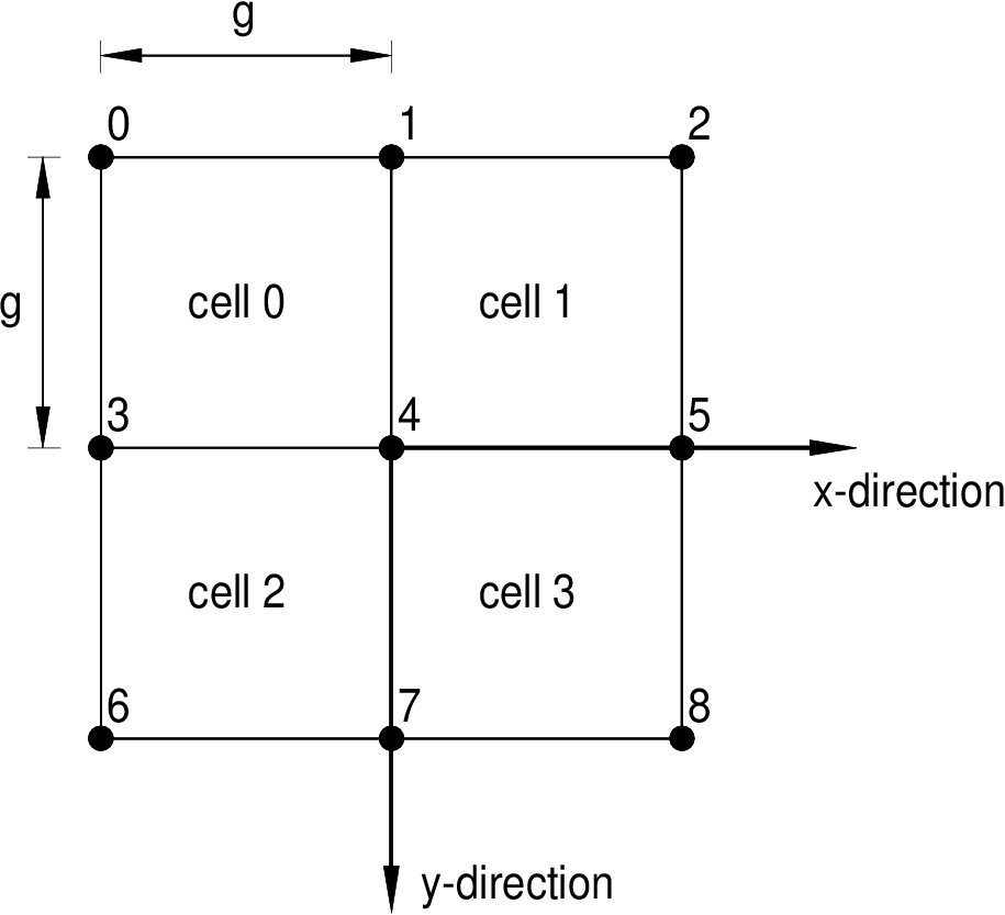
The correlation between the collected charges at the
particular nodes and the reconstructed event positions
can be realized for the
particular algorithms in the - and -direction as follows:
4-node algorithm (events somewhere in cell 1; ) :
| (1) | ||||
6-node algorithm (node 1 and 4 (node 4 and 5) carry maximum signal for reconstruction in -direction (-direction); and ):
| (2) | ||||
3-node algorithm (node 4 carries maximum signal; ):
| (3) | ||||
The sum of the collected charges in - and -direction of the particular algorithms are abbreviated with , , , and . The higher the ratio of the more pronounced is the cell like character and the electrical screening among the cells. This leads to a treatment of the readout structure consisting of strongly separated cells which makes the application of the 4-node algorithm stressing this cell structure most favourable. In practise the charge screening of the cells is always finite. Therefore, the application of other algorithms featuring symmetry planes at the cell border (6-node algorithm) and the readout node (3-node algorithm) is sensible.
The most simplest algorithm imaginable is the 2-node algorithm. But since this algorithm only takes two nodes into account it is strongly affected by systematic effects (like cross-talk or variations of the amplification of the preamplifiers). Therefore, the 2-node algorithm, when applied in practise, is inferior to the other algorithms and is not further considered.
3.3 Reconstruction properties of the linear algorithms
3.3.1 Position reconstruction
By means of the -cell diffusion simulation it is possible to investigate the reconstruction behaviour of the three algorithms. A series of individual simulations has been carried out impinging a short driving current successively at every grid point (homogeneous grid point spacing ). All positions are calculated after the 25 nodes of the -cells have collected almost of the impinged charge. Altogether one obtains therefore possible positions within one single cell.
In Fig. 3 the reconstructed positions of the 4-, 6- and 3-node algorithm are shown within a cell for .

The 4-node algorithm shows large distortions close to the cell borders which means large deviations between the elements of the two spaces and , whereas this algorithm is nearly distortion free in the centre of a cell. On the other hand both the 6-node and the 3-node algorithm have their maximum distortions in the cell centre. Close to the cell borders they are more favourable for position reconstruction since their distortions are much smaller compared to the 4-node algorithm. Obviously, the reconstruction behaviour of the 6- and the 3-node algorithm is quite similar, since they use comparable symmetry planes and readout nodes.
For a homogeneous input illumination – we impinged charges on every grid point – a perfect reconstruction algorithm would result in a homogeneous output population density. Since none of the introduced algorithms is a perfect reconstruction algorithm (s. Fig. 3) variations in the population density become obvious. Mathematically the correlation between the true positions and the reconstructed positions is given by a two-dimensional Jakobi-determinant (coordinate transformation), which correlates the two population densities and :
| (4) |
Therfore, we obtain
| (5) | ||||
with the Jakobi-determinant :
| (6) | ||||
whereby the second relationship for can be derived by the back-transformation . The derivatives with respect to the true positions and are easier to calculate in a numerical fashion since the positions are placed on an equidistant lattice in the case of a homogeneous illumination. Therefore the second relationship for from Eq. (6) is used for further numerical calculations.
A homogeneous illumination like in this simulation means which is set in the following (arbitrarily) to . This leads to (Eq. (5)). In Fig. 3 the relationship between the true positions and the reconstructed positions is shown for quantised distances. It is obvious that is unequal to one which directly leads to an inhomogeneous population density . This is also visible by the variation of the density of the black points in Fig. 3. A higher density of points is equivalent to a higher population density . In Fig. 4 the population density for the 4-node algorithm is shown as an example.

A perfect algorithm which connects the reconstructed positions with the true positions and by and would lead to a population density .
Unfortunately, it is a non-trivial task to find a suitable transformation between the two spaces and since the functions and are explicitly needed. Starting with one of the linear algorithms (e.g. the 4-node algorithm) one will end up in major problems: Since all the data were calculated numerically with a finite grid spacing (e.g. ) one has to approximate the functions and e.g. by polynomials or Fourier series to get an analytical approach. Thereby, it showed up that one has to take too many orders into account to decrease the deviation between positions reconstructed by the simulation and the polynomials. But even if there exists a satisfying solution of an analytical expression for and another much more serious problem arises. One has to take carefully the spatial resolution into account. As it will be seen later on, the transformation for and , which will correct the reconstructed positions , will dramatically deteriorate the spatial resolution at the positions where larger corrections have to be applied. This will be for example the case at the cell borders when using the 4-node algorithm where we have larger population densities (s. Fig. 4) and therefore larger position corrections.
Also the access via a direct measurement is closed since an extensive mechanical scan has to be done; e.g. by means of a fine needle impinging a certain amount of charge onto the readout structure. At least one has to scan – depending on the desired accuracy – a few thousand positions which will lead to an enormous effort. Besides, the true positions are hard to determine due to the finite mechanical accuracy of the setup.
3.3.2 Spatial resolution
In most position sensitive detector systems the spatial resolution represents an important parameter which has to be optimised depending on the desired application. Since in interpolating systems like in our case the reconstruction algorithms themselves affect the spatial resolution additionally (besides e.g. the signal-to-noise ratio (SNR) or the pixel-size for pure pixel detectors), the influence of the algorithms has to be analysed separately in this respect.
The absolute values of the spatial resolution of the different algorithms are determined by the SNR. Since the spatial resolution of all algorithms is (s. b.) the absolute noise resistance is not explicitly needed when the various algorithms are compared to each other. In the following we treat the parallel noise of the readout structure as the dominant noise source, which mainly determines the spatial resolution. Every readout node collecting the charge is subjected to Nyquist-Johnson noise
| (7) |
with denoting the charge integration time. Thereby, the collected charge including the noise contribution is normally distributed around . For the total spatial resolution the electronic noise would also have to be considered. It has deliberately not been included in the calculations to leave the discussion independent from the electronics used. For most practical cases it will be in the same order of magnitude or smaller than the noise contribution, presented here.
Taking into account the particular algorithms (Eqs. (1)–(3)) and assuming a constant gaussian charge noise (Eq. (7)) error propagation leads to the spatial resolution in -direction:
| (8) |
where and indicate the true event position (impact position) upon the readout plane and the charge integration time, respectively. The calculation in -direction behaves correspondingly. The sum runs over all participating nodes of the particular algorithms. Since some charges appear both in the - and the -coordinate the two coordinates are correlated. Therefore, the noise causes a spatial smearing which can be expressed by a two-dimensional gaussian distribution with describing the strength of the correlation (e.g. [16]):
| (9) | ||||
For the 4-, 6- and 3-node algorithms one obtains for the spatial uncertainty (corresponding coordinate systems s. Fig. 2):
4-node algorithm:
| (10) | ||||
6-node algorithm:
| (11) | ||||
3-node algorithm:
| (12) | ||||
The cell size is denoted by . Again the reconstructed positions are indicated by together with a number as a subscript for the particular algorithm. The terms of the spatial resolutions can be separated into a geometrical factor and a factor consisting of the SNR. Fig. 5 shows schematically the results of the spatial resolutions (fwhm) as a function of the distorted reconstructed position for all three algorithms within a single -cell taking both the geometrical factor and the SNR-factor into account.

Obviously, the 4-node algorithm shows up to be the most favourable algorithm since it provides the best spatial resolution. Since the 3-node algorithm collects in the cell centre only about half of the impinged charge the SNR-factor decreases and therefore the spatial resolution deteriorates in comparison to the other algorithms. Only at the nodes the spatial resolution for the 3- and the 4-node algorithm becomes similar, since the geometric factors (cf. Eqs. (10) and (12)) and the SNR-factors are the same.
Actually, the spatial resolution in Fig. 5 is plotted as a function of the reconstructed positions and not of the true positions . If one corrects the reconstructed positions by means of a coordinate transformation which transforms the spatial resolution of the corrected positions can be estimated by:
| (13) | ||||
Eq. (13) determines the spatial resolution of the corrected positions as a function of the covariance, the spatial resolutions and of the applied algorithm (cf. Eqs. (10)–(12)) and the derivatives between the coordinates and . In this equation all appearing should be treated as . Fig. 6 shows exemplarily the numerically calculated spatial resolution (fwhm) obtained by Eq. (13) as a function of the true positions for the 4-node algorithm.

Since at the cell borders where the population density of all algorithms is relatively high (s. Fig. 3) larger corrections have to be applied the spatial resolution deteriorates by almost a factor of – for all algorithms.
3.4 Introduction of the optimised 463-node algorithm
In the following we present a possible solution which takes care of both the correct position reconstruction and the spatial resolution, by combining the 4-, 6- and 3-node algorithms to one 463-node algorithm.
All algorithms converting a homogeneous population density into an inhomogeneous population density which is equivalent to a wrong position reconstruction are not favourable. Even for the case of a later position correction these algorithms will always suffer from a bad spatial resolution at the positions where larger position corrections have to be applied (cf. end of Sec. 3.3.2). Therefore, it would be much more advantageous to find an algorithm which is capable to reconstruct almost the correct positions which require only small subsequent position corrections and which therefore only weakly influence the spatial resolution. The idea of combining the 4-, 6- and 3-node algorithm to the 463-node algorithm shows up to be a possible solution fulfilling almost the requirements mentioned above.
Based on the results of the simulation model giving a relationship between and the combination of the algorithms in -direction is done by mixing matrices and , defined for every grid point in the cell. The elements mix the 4-node algorithm continuously with either the 6-node or the 3-node algorithm, whereby the elements of the second mixing matrix consisting only of the values 0 or 1 choose either the 6-node () or the 3-node () algorithm. The following equation defines the complete 463-node algorithm, whereby and are those elements of the matrices corresponding to the true position . The origin of the 4-node algorithm is now shifted to readout node 4 (cf. Fig. 2):
| (14) | ||||
For symmetry reasons the relationship between the mixing matrices in - and -direction is simply: and . The procedure for the combination of and is shown in the schematic diagram in Fig. 7.

In the following the derivation of the matrices and is discussed for the -direction. The -direction behaves correspondingly.
The spatial resolution and of the 6- and the 3- node algorithm is the criterion for the matrix with (cf. Eqs. (11) and (12)). If the 6-node algorithm is used (); if the 3-node algorithm is used (). Since the deviations between the reconstructed positions of the 6-node and the 3-node algorithm are small (s. Fig. 3) also the influence of the points of discontinuity () is expected to be negligible.
The criterion for the combination between the 4-node and the 6- or the 3- node algorithm is an optimised position reconstruction which means a minimum deviation between and . Together with we get as a criterion:
| (15) |
whereby again and . The minimum condition leads to . Since the criterion for a minimum is fulfilled. As a result we obtain for the matrix elements :
| (16) |
The constraint
| (17) |
has to be set because for some positions mixing factors would end up in additional distortions due to noise or systematic effects (cf. Sec. 4). Consequently, this constraint leads to the fact that some positions are still not reconstructed correctly.


The 4-node algorithm determines already the optimum positions in -direction close to the low resistivity cell borders (except close to the readout nodes), therefore it is the only algorithm applied (). In -direction close to the cell borders the 4-node algorithm becomes unfavourable (cf. Fig. 3 a)) and the other participating algorithms are more emphasised (). As expected the 6-node algorithm offers the best spatial resolution close to the symmetry axis of the cell, whereas the 3-node algorithm becomes more favourable in -direction close to the low resistivity cell borders and the readout nodes (cf. also Fig. 5). Fig. 10 shows the reconstructed positions obtained with the 463-node algorithm by means of Eq. (14).

The slight distortions for some positions mainly close to the nodes are due to the constraint in Eq. (17) and can be directly revealed in the population density plot (Fig. 11). A very slight inhomogeneity is also visible close to the low resistivity strips at the cell borders. In comparison with the population density of the 4-node algorithm (Fig. 4) the population density of the 463-node algorithm is nearly flat and especially close to the cell borders and the readout nodes improved by a factor 2–4.

Besides this as a consequence also the spatial resolution is improved. In Fig. 12 the spatial resolution of the 463-node algorithm is plotted as a function of the reconstructed positions .

In fact the error propagation (Eq. (8) and Eq. (14)) leads for the 463-node algorithm to a non-trivial equation for the spatial resolution. However, as expected due to the mixing matrices and close to the nodes and the cell borders in -direction the spatial resolution is comparable to that obtained by the single 3-node and 6-node algorithm (cf. Fig. 5). Close to the cell borders in -direction the behaviour of the single 4-node algorithm is reflected. Since the positions are indeed well reconstructed (Fig. 10) the spatial resolution of the 463-node algorithm as a function of the true positions is very similar to that of the reconstructed positions (Fig. 12). Only close to the nodes the spatial resolution is slightly deteriorated caused by the small position corrections (s. Eq. (13)).
3.5 Application of the 463-node algorithm on measured data
The application of the 463-node algorithm (Eq. 14) demands for the mixing matrices and . Since these matrices are actually a function of the true positions which are not known a priori in a measurement we have to apply an iterative technique. To obtain a first approximate position an assumption for suitable elements and is needed. For that reason the reconstructed position is calculated firstly both by means of the -node and the 4-node algorithm. At a distance of (with as the cell size) around the cell borders the -node algorithm is used for a first estimation of to obtain the matrix elements and . Else the 4-node algorithm is used for the estimation of and . Then, the 463-node algorithm position is calculated for the first time, which gives new positions and therefore an estimation of new and . This iterative procedure is repeated several times until the reconstructed positions converge. Since the diffusion simulation gives matrices and with elements corresponding to a grid spacing of (Figs. 8 and 9) we have used an interpolation routine of IDL [17] to achieve a finer resolution. If the virtual pixel size is e.g. chosen to we use finer matrices and with elements, corresponding to grid spacing to allow a better convergence of the 463-node algorithm. Since this method converges at almost all positions within the cell this iterative loop is used for all image reconstructions of measured data presented in the following.
Fig. 13 shows the response of the inner cells () of a detector with a PCB-readout structure to an uniform illumination () reconstructed with the 4-node algorithm (Eq. 1).

A -source has been used for illumination (). The detector has been operated with an (90/10) gas filling at standard pressure.
The low resistivity cell borders of the PCB-structure have a width of about . The special resistive materials used for the silk-screen printing process have surface resistances of and , respectively. Unfortunately the printing and burning processes have a strong influence on the resistances and the exact ratio of is hardly predictable. Since the depletions at the cell borders when using the 4-node algorithm show a good regularity in all cells (Fig. 13) we conclude that the relative accuracy of the surface resistances is in the percent range. The resulting image when using the 463-node algorithm is shown in Fig. 14.

The matrices and are created for and since this ratio simply fits best, whereby the distortions of the 4-node algorithm depend less than linear on the ratio . This means that one obtains e.g. only little changes concerning the distortions when treating a ratio of instead of . The population density becomes much more homogeneous in comparison to the 4-node algorithm. In addition the standard deviation of the intensity per pixel is dramatically reduced from to which is indeed much closer to the theoretical limit of .
4 Non-linear corrections
Although the reconstructed image with the 463-node algorithm (Fig. 14) represents a mentionable progress compared to images reconstructed e.g. with the 4-node algorithm (Fig. 13) still some inhomogeneities in the population density are obvious. These artifacts can mainly be attributed to systematic effects (which partly occur during the measurement). As already described, even in the theoretical case the 463-node algorithm leads to a slight overpopulation close to the cell borders and especially around the nodes (cf. Fig. 11). Systematic electronic effects, like gain variations of the preamplifiers and cross-talk in the preamplifiers/cables can possibly influence the image. Besides this, a too short integration time of the preamplifiers can lead to an overpopulation (as can be shown by simulations) of the cell borders. Further systematic effects stem from the readout structure itself, like the finite dimensions of the readout nodes, the finite accuracy of the width of the low resistivity strips and local inhomogeneities of the surface resistances.
4.1 Homogeneous population density
In order to decrease the remaining inhomogeneities around the readout nodes and the cell borders (cf. Fig. 14) an ansatz is made for and , whereby the abbreviation and is used in the following. Since we know that the incident population density for a homogeneous illumination is equal to unity Eq. (5) reads as follows:
| (18) |
The functions and have now to be optimised in such a fashion that the derivatives correspond to the measured population density . Fig. 15 shows the measured mean population density obtained by the superposition of the cells shown in Fig. 14.

The mean value of is normalised to unity; also the cell size is normalised to one (). We have composed the coordinate transformation functions and by suitable combinations of different one- and two-dimensional Gaussian functions with the cell centre as the point of symmetry. The final coordinate transformation functions and have altogether 6 independent parameters. Fig. 16 shows the population density as a result of the minimisation of .

The measured population density (Fig. 15) and the population density obtained by the coordinate transformation functions and (Fig. 16) are in good agreement. The knowledge of and allows now to correct for the small inhomogeneities around the nodes and the cell borders. By this procedure, the reconstructed positions of the 463-node algorithm are transformed into the corrected positions and . Fig. 17 shows the resulting non-linear corrected image.

The standard deviation of the intensity per pixel is further reduced from (Fig. 14) to which is even closer to the theoretical limit of .
4.2 Inhomogeneous population density
Since all assumptions made in the previous sections are based on a homogeneous population density we have to test the 463-node algorithm (Sec. 3.4) and the corresponding non-linear corrections separately with an inhomogeneous population density. This can e.g. be performed with a suitable collimator. More images (even time-resolved measurements) in the field of biological and chemical diffraction samples recorded with the ViP-detector prototype can be found in Ref. [12].
Fig. 18 shows the image of a laser cut thick stainless steel aperture containing “SAXS 2D” letters (Small Angle X-ray Scattering) and five holes with increasing hole diameters.

The image has been recorded with a PCB-readout structure using photons of an energy of (fluorescence of a Fe-target in a synchrotron beam). The detector was filled with a (90/10) gas mixture at a pressure of . The image has been reconstructed with the linear 463-node algorithm with subsequent non-linear corrections at the nodes and at the cell borders. We performed an additional flatfield correction with a flatfield image recorded in our laboratory one week after the aperture measurement with a different gas filling and a different X-ray source. Since this flatfield image is different from one which we would have obtained at the beamline directly after the aperture measurement (with identical detector parameters), the corrected image still shows up some artifacts like visible areas around the readout nodes (marked with dotted lines) which should have been suppressed by the correction of the proper flatfield image.
However, the recorded image compares well to the image of the aperture (right hand side image in Fig. 18). Only the middle part of the second “S” (dashed line) looks slightly distorted; at this readout channel the preamplifier was not working optimally (compare to uppermost dotted circle in Fig. 14). Also the reproduction of the holes shows a good agreement.
5 Conclusion
The simplest linear algorithms do not reconstruct the event positions correctly. This leads to distortions since the true positions and the reconstructed positions differ up to a certain extent. When these algorithms are corrected afterwards by a suitable coordinate transformation connecting the two spaces and the spatial resolution becomes worse especially next to the cell borders and the readout nodes.
Therefore, the 463-node algorithm is introduced. This complex algorithm consisting of combinations of linear algorithms is a possible solution for position reconstructions using the two-dimensional interpolating resistive readout structure described above. This algorithm has been optimised with respect to both the correct position reconstruction and the spatial resolution. Indeed, the reconstruction of a homogeneous population density as a measure for the quality of an image has been considerably improved – even close to the Poisson limit – when the 463-node algorithm with subsequent non-linear corrections was applied. Nevertheless, some inhomogeneities mainly caused by systematic effects are still visible in the images. Since these disturbing effects can not be corrected afterwards they should be kept as small as possible.
References
- [1] A. Bressan, R. De Oliveira, A. Gandi, J.-C. Labbé, L. Ropelewski, F. Sauli, D. Mörmann, T. Müller, H. J. Simonis, Two-dimensional readout of GEM detectors, Nucl. Instr. and Meth. A425 (1999) 254–261.
- [2] S. Bachmann, S. Kappler, B. Ketzer, T. Müller, L. Ropelewski, F. Sauli, E. Schulte, High rate X-ray imaging using multi-GEM detectors with a novel readout design, Nucl. Instr. and Meth. A478 (2002) 104–108.
- [3] J. P. Cussonneau, M. Labalme, P. Lautridou, L. Luquin, V. Metivier, A. Rahmani, T. Reposeur, 2D localization using resistive strips associated to the Micromegas structure, Nucl. Instr. and Meth. A492 (2002) 26–34.
- [4] R. Lewis, Multiwire Gas Proportional Counters: Decrepit Antiques or Classic Performers?, J. Synchrotron Rad. 1 (1) (1994) 43–53.
- [5] H. J. Besch, M. Junk, W. Meißner, A. Sarvestani, R. Stiehler, A. H. Walenta, An interpolating 2D pixel readout structure for synchrotron X-ray diffraction in protein crystallography, Nucl. Instr. and Meth. A392 (1997) 244–248.
- [6] F. Sauli, GEM: A new concept for electron amplification in gas detectors, Nucl. Instr. and Meth. A386 (1997) 531–534.
- [7] Y. Giomataris, P. Rebourgeard, J. P. Robert, G. Charpak, MICROMEGAS: a high-granularity position-sensitive gaseous detector for high particle-flux environments, Nucl. Instr. and Meth. A376 (1996) 29–35.
- [8] F. Bartol, M. Bordessoule, G. Chaplier, M. Lemonnier, S. Megtert, The C.A.T. Pixel Proportional Gas Counter Detector, J. Phys. III France 6 (1996) 337–347.
- [9] A. Sarvestani, H. J. Besch, M. Junk, W. Meißner, N. Sauer, R. Stiehler, A. H. Walenta, R. H. Menk, Study and application of hole structures as gas gain devices for two dimensional high rate X-ray detectors, Nucl. Instr. and Meth. A410 (1998) 238–258.
- [10] A. Orthen, H. Wagner, H. J. Besch, R. H. Menk, A. H. Walenta, U. Werthenbach, Investigation of the performance of an optimised MicroCAT, a GEM and their combination by simulations and current measurements, Nucl. Instr. and Meth. A500 (2003) 163–177.
- [11] A. Orthen, H. Wagner, H. J. Besch, S. Martoiu, R. H. Menk, A. H. Walenta, U. Werthenbach, Gas gain and signal length measurements with a triple-GEM at different pressures of Ar-, Kr- and Xe-based gas mixtures, Nucl. Instr. and Meth. A512 (2003) 476–487.
- [12] A. Orthen, H. Wagner, S. Martoiu, H. Amenitsch, S. Bernstorff, H. J. Besch, R. H. Menk, K. Nurdan, M. Rappolt, A. H. Walenta, U. Werthenbach, Development of a two-dimensional virtual pixel X-ray imaging detector for time-resolved structure research, submitted to J. Synchrotron Rad. (2003).
- [13] A. Sarvestani, N. Sauer, C. Strietzel, H. J. Besch, A. Orthen, N. Pavel, A. H. Walenta, R. H. Menk, Microsecond time-resolved 2D X-ray imaging, Nucl. Instr. and Meth. A465 (2001) 354–364.
- [14] S. Martoiu, A. Orthen, H. Wagner, H. J. Besch, R. H. Menk, K. Nurdan, A. H. Walenta, U. Werthenbach, Intelligent local trigger technique for a multi-cell 2D interpolating resistive readout, to be submitted to Nucl. Instr. and Meth. A (2003).
- [15] H. Wagner, H. J. Besch, R. H. Menk, A. Orthen, A. Sarvestani, A. H. Walenta, H. Walliser, On the dynamic two-dimensional charge diffusion of the interpolating readout structure employed in the MicroCAT detector, Nucl. Instr. and Meth. A482 (2002) 334–346.
- [16] S. Brandt, Data Analysis, Spinger, New York, 1999.
- [17] IDL 5.3, Research Systems Inc., Boulder, CO, USA.