Preprint of:
T. A. Nieminen, H. Rubinsztein-Dunlop and N. R. Heckenberg
“Multipole expansion of strongly focussed laser beams”
Journal of Quantitative Spectroscopy and Radiative Transfer
79–80, 1005–1017 (2003)
Multipole expansion of strongly focussed laser beams
T. A. Nieminen, H. Rubinsztein-Dunlop, and N. R. Heckenberg
Centre for Biophotonics and Laser Science, Department of Physics,
The University of Queensland, Brisbane QLD 4072, Australia
timo@physics.uq.edu.au
Abstract
Multipole expansion of an incident radiation field—that is, representation of the fields as sums of vector spherical wavefunctions—is essential for theoretical light scattering methods such as the T-matrix method and generalised Lorenz-Mie theory (GLMT). In general, it is theoretically straightforward to find a vector spherical wavefunction representation of an arbitrary radiation field. For example, a simple formula results in the useful case of an incident plane wave. Laser beams present some difficulties. These problems are not a result of any deficiency in the basic process of spherical wavefunction expansion, but are due to the fact that laser beams, in their standard representations, are not radiation fields, but only approximations of radiation fields. This results from the standard laser beam representations being solutions to the paraxial scalar wave equation. We present an efficient method for determining the multipole representation of an arbitrary focussed beam.
Keywords: nonparaxial beams; light scattering; optical tweezers; localized approximation; expansion coefficients; shape coefficients
PACS: 42.25.Bs, 42.25Fx, 42.60.Jf
1 Introduction
Multipole expansion of an incident radiation field in terms of vector spherical wavefunctions (VSWFs) is required for theoretical scattering methods such as the T-matrix method [1, 2, 3] and generalised Lorenz-Mie theory (GLMT) [4]. Since the VSWFs are a complete orthogonal basis for solutions of the vector Helmholtz equation,
| (1) |
it is theoretically straightforward to find the multipole expansion for any monochromatic radiation field using the orthogonal eigenfunction transform [5, 6], also known as the generalised Fourier transform. For example, the usual formula for multipole expansion of a plane wave can be derived in this way.
While the case of plane wave illumination is useful for a wide range of scattering problems, many applications of scattering involve laser beams. In particular, laser trapping [7] requires strongly focussed beams. As scattering calculations allow the optical forces and torques within the optical trap to be determined [8, 9], and the T-matrix method is particularly useful for the repeated calculations typically required, multipole expansion of laser beams, including strongly focussed beams, is extremely useful.
Unfortunately, laser beams present some serious theoretical difficulties. These problems are not a result of any deficiency in the basic process of multipole expansion of radiation fields, but are due to the fact that standard representations of laser beams are not radiation fields—that is, their standard mathematical forms are not solutions of the vector Helmholtz equation, but are solutions of the paraxial scalar wave equation (higher order corrections can be used to improve the accuracy as reality becomes less paraxial [10]). Such pseudo-fields are only approximate solutions of the vector wave equation. The deviation from correctness increases as the beam is more strongly focussed [11, 12, 13].
While, in principle, any radiation field can be expanded in terms of multipoles, multipole expansions do not exist for approximate pseudo-fields that do not satisfy the vector wave equation. Since the standard paraxial representations of laser beams are so widely used, multipole expansions that correspond to the standard beams in a meaningful way are highly desirable. For this to be possible, some method must be used to “approximate” the standard laser beam with a real radiation field. We can note that there exists a significant and useful body of work on multipole expansion of beams [14, 15, 16, 17, 18, 19, 20]. However, while satisfactorily efficient and accurate methods exist for weakly focussed beams, when the deviations from paraxiality are small, strongly focussed beams, for example, as required for laser trapping, remain problematic.
The traditional method used in scattering calculations was to assume that the actual incident field was equal to the paraxial field on the surface of the scatterer. This has the unfortunate drawback that the multipole expansion coefficients depend on the size, shape, location, and orientation of the scattering particle. As a result, an artificial dependence on particle position and size is introduced into scattering calculations and calculations of optical forces, since the differing multipole expansions correspond to different beams. This is obviously undesirable. While matching the fields on the surface of the scattering particle is not an adequate solution to the problem, the basic concept—matching the fields on a surface—is sound. However, a scatterer-independent surface must be used. Two natural choices present themselves: the focal plane (for beams with a well-defined focal plane), and a spherical surface in the far field.
Integral methods can be used over these surfaces (direct application of the orthogonal eigenfunction transform). Here, however, we use a point-matching method since, firstly, the method tolerates a much coarser grid of points, thereby increasing computational efficiency, and secondly, increased robustness can be gained by using extra points to give an overdetermined system of equations which can then be solved in a least-squares sense. We use both focal plane matching and far field matching, and evaluate their respective merits.
2 Point-matching method
All monochromatic radiation fields satisfy the vector Helmholtz equation (1) in source-free regions. The vector spherical wavefunctions (sometimes called vector spherical harmonics) are a complete set of orthogonal solutions to this equation. The VSWFs are
| (2) | |||||
| (3) | |||||
where are spherical Hankel functions of the first and second kind, are normalisation constants, and , , and are the vector spherical harmonics:
| (4) | |||||
| (5) | |||||
| (6) |
where are normalised scalar spherical harmonics. The usual polar spherical coordinates are used, where is the co-latitude measured from the axis, and is the azimuth, measured from the axis towards the axis. The term in (3) results from the identity .
and are outward-propagating TE and TM multipole fields, while and are the corresponding inward-propagating multipole fields. Since these wavefunctions are purely incoming and purely outgoing, each has a singularity at the origin. Since the incident field has equal incoming and outgoing parts, and must be singularity free in any source-free region, it is useful to define the singularity-free regular vector spherical wavefunctions:
| (7) | |||||
| (8) |
Since the spherical Bessel functions , the regular VSWFs are identical to the incoming and outgoing VSWFs except for the replacement of the spherical Hankel functions by spherical Bessel functions.
Since the VSWFs are a complete set of solutions to the vector Helmholtz equation (1), every solution can be written as a linear combination of VSWFs. Thus, the incident field can be written in terms of expansion coefficients (also called beam shape coefficients) and as
| (9) |
Alternatively, since the outgoing field is purely a consequence of the incoming field (with or without a scatterer present), all the necessary information can be conveyed by writing the incident field expansion in terms of incoming wavefunctions as
| (10) |
The two sets of expansion coefficients are related, since and (the scattered/outgoing field expansion coefficients will differ). In practice, the multipole expansion will be terminated at some . For the case of multipole fields produced by an antenna that is contained within a radius , is usually adequate, but is advisable if higher accuracy is needed [21]. This can also be used as a guide for choosing for beams—if the beam waist is contained in a radius , this can be used to choose . Since the multipole field necessarily deviates from the paraxial field, the required accuracy is open to question. It appears that generally gives adequate results.
For focal plane matching of the fields, the regular wavefunctions are used, while for far field matching, the incoming wavefunctions are used. The use of only the incoming portion of the field for matching the fields in the far field means that no knowledge of the outgoing portion of the fields is required.
If the field expansion is truncated at , equation (9) or (10) contain unknown variables—the expansion coefficients and . They can be found from a set of equations. If we know the field at enough points in space, either by using the standard paraxial form of the beam, or from measurements, a sufficiently large set of equations can be generated. Since the electric field has three vector components at each point in space, three equations result from each point. For robustness, extra points can be used to give an over-determined linear system which can then be solved in a least-squares sense. This is the basic point-matching procedure. The point spacing along any spherical coordinate must be sufficient to prevent aliasing of the VSWFs with respect to that coordinate.
The linear system can be written as a matrix of size , so solution of the system will scale as . While this is clearly less desirable than integral methods which scale as for surface methods and for volume methods, integral methods require a much more closely spaced grid of points. Since we are mainly interested in strongly focussed beams, when is small, the gain in speed through the use of a coarse grid results in improved performance. We can note that the most efficient solution to very wide beams is simply to approximate them as plane waves (an solution), which will be quite adequate if the scattering particle is small compared to the beam width, and located near the beam axis. Optimisations for axisymmetric beams, giving performance, are described later.
3 Focal plane matching
Point-matching in the focal plane offers a number of advantages. Firstly, the paraxial beam has a simple phase structure in the focal plane. Secondly, the focal plane is likely to be the region in which scattering or trapping takes place. Thirdly, the irradiance distribution in the focal plane may be known experimentally. Although an accurate measurement of the focal plane irradiance distribution is usually quite difficult, due to the finite resolution of typical detectors, the structure of the beam, and the approximate focal spot size, can be determined. The major disadvantage is that the greatest differences between the paraxial beam and the real beam can be expected to occur in the focal plane. For example, a paraxial beam has zero longitudinal components of the electric field, but, from Maxwell’s equations, the longitudinal component must be non-zero.
For mathematical convenience, we choose a coordinate system so that the beam axis coincides with the axis, with the beam propagating in the direction, with the focal plane coincident with the plane (the plane). Next, we can generate a grid of points, and calculate the electric field components of the paraxial beam at these points.
A practical difficulty immediately presents itself, however, since the spherical harmonics with odd are odd with respect to , and will be zero for —the focal plane. This is to be expected physically, since the same electric field amplitude in the focal plane can correspond to a beam propagating in the direction, the direction, or a standing wave created by the combination of these. A mathematically rigorous way of dealing with this is to match the derivatives of the electric field amplitude, as well as the field amplitude itself. However, this isn’t necessary, since we have already chosen a direction of propagation as one of the initial assumptions. Therefore, it is sufficient, and computationally efficient, to use only those VSWFs that will be non-zero to determine the corresponding “missing” expansion coefficients. This will give half of the required expansion coefficients. Then, from the direction of propagation, or gives the “missing” coefficients. If the beam propagates in the direction, or are used. If the beam was a pure standing wave combination of counter-propagating beams, these expansion coefficients would be zero.
In principle, this procedure can be carried out for an arbitrary beam. However, determining the vector components of beams where the Poynting vector is not parallel to the axis in the focal plane will be problematic, since there will be no unique choice of electric field direction since the paraxial beam is also a scalar beam. Therefore, we will restrict ourselves to beams with -directed focal plane Poynting vectors only. This eliminates, for example, Laguerre-Gaussian beams LGpl with .
Often, the beam of interest will have an axisymmetric irradiance distribution. Any beam that can be written as a sum of Laguerre-Gaussian modes LGp0 will satisfy this criterion. The most significant such beam is the TEM00 Gaussian beam (which is also the LG00 beam). Beams with these properties have only multipole components [15, 16], which follows simply from the dependence of the VSWFs. This allows a significant computational optimisation, since only the VSWFs need to be included in the point-matching procedure. This results in performance.
The point-matching procedure described above was implemented using MATLAB [22]. Since the main computational step is the solution of an overdetermined linear system, a linear algebra oriented language/system such as MATLAB was natural choice. Additionally, existing MATLAB routines for the calculation of Bessel, Hankel, and associated Legendre functions allow simple calculation of VSWFs. Since the VSWFs only need to be calculated for , a special purpose fast VSWF calculation routine could be used.
3.1 TEM00 beam
The scalar amplitude of a TEM00 Gaussian beam is given in cylindrical coordinates by [23]
| (11) |
where is the wavenumber, is the waist radius, is the central amplitude, is the complex radius of curvature, and where is the Rayleigh range. In the focal plane, and the above expression can be slightly simplified. For a beam linearly polarised in the direction, and , while for circularly polarised beams, and . in all cases.
The general structure of a real beam point-matched with a TEM00 Gaussian beam of waist radius is shown in figure 1. The beam is very similar to those given by Gouesbet’s localised approximation [15, 16, 19], although the (very small) component is somewhat different. The robustness of the algorithm is shown by the generation of the correct components for the final beam, even though the original paraxial beam was unphysically assumed to have .

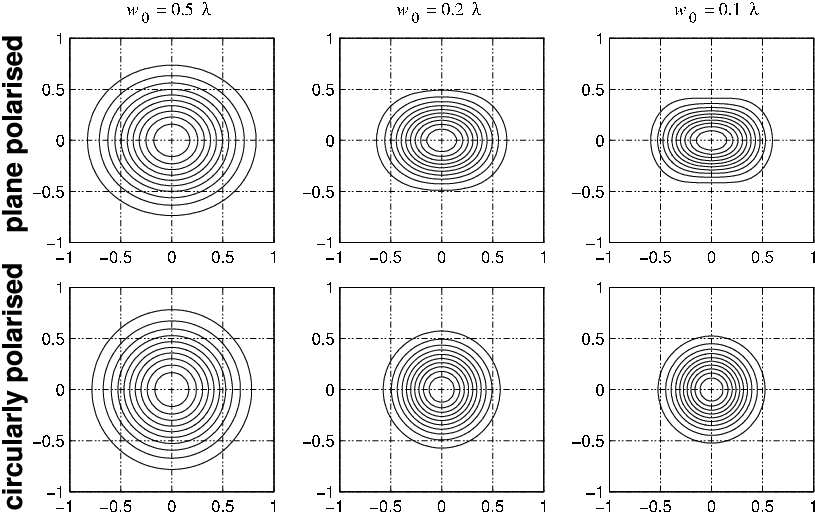
The behaviour of the beam as it is more tightly focussed is shown in figure 2. The increasing axial asymmetry of plane-polarised beams as they are more strongly focussed can be clearly seen. The other feature to note is that focussed beams have a minimum waist size—the more strongly focussed beams shown here closely approach this minimum size, the well-known diffraction limited focal spot [23, 24, 25]. The lack of any such limit in the paraxial beam is blatantly unphysical, and we cannot expect a beam matched to a paraxial beam to have such an unreasonably small waist radius.
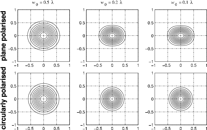
The for these calculations was determined by assuming that an effective radius of contains the entire beam in the focal plane. This gives , 9, and 6 for the three beam widths of , , and . All VSWFs were included in the solution (that is, the axisymmetric beam optimisation was not used), so the number of unknown variables for each case was 576, 198, and 96. The fields were matched at a number of points equal to the number of variables, distributed on a polar grid. This is an overdetermined system, with 50% more points than required. The times required for the solution of the linear system on a 1.5 GHz PC were 11.2 s, 0.50 s, and 0.046 s, respectively. If the solution is restricted to the VSWFs, the number of variables is reduced to , and the times required for the three cases shown are reduced to 0.006 s, 0.002 s, and 0.001 s.
3.2 Bi-Gaussian beam
We consider a simple non-axisymmetric beam, constructed by replacing in the paraxial Gaussian beam formula (11) by , giving a bi-Gaussian irradiance distribution with an elliptical focal spot. The expansion coefficients are no longer restricted to .
The irradiance distributions of point-matched bi-Gaussian beams are shown in figure 3. The effect of the minimum spot size is evident, as it first restricts the focussing in the direction, and then the direction, as the beam is more strongly focussed. The odd multipole components are non-zero in these beams. The increased width of the beam results in longer calculations using the cutoff radius. A smaller cutoff radius equal to produces very similar results, and may be more suitable for practical use. Since the non-zero expansion coefficients can be predicted from the symmetry of the beam, it would also be possible to speed up the calculations by only including those coefficients.

4 Far field matching
In the far field, the beam becomes an inhomogeneous spherical wave. The radial component of the electric and magnetic fields vanishes. The large radius limits for the VSWFs [3]:
| (12) | |||||
| (13) |
can be usefully employed. The far field is best written in spherical polar coordinates, since this gives at most two non-zero components. In cartesian coordinates, all three components will generally be non-zero, although only two will be independent. Since only two vector components of the field can be used in the point matching procedure, the minimum number of points at which to match the fields that is needed is higher.
The non-zero spherical polar vector components of the far field beam can be obtained from the paraxial scalar expressions for the two plane polarised components and :
| (14) | |||||
| (15) |
4.1 TEM00 beam
The far field spherical wave limit of the paraxial Gaussian beam formula (11) can be found by converting the cylindrical coordinates to spherical coordinates and taking the large limit, giving
| (16) |
Focal plane irradiance contours for far field matched beams are shown in figure 4. Except for the use of the far field for matching, the procedure, and the results, are the same as the focal plane matching case.
4.2 LGpl beams
We recall that the focal plane matching procedure is greatly complicated when the Poynting vector in the focal plane is not parallel to the beam axis, and note that the same does not apply to far field matching—the Poynting vector is always purely radial in the far field regardless of its behaviour in the focal plane. Therefore, beams of these types, such as Laguerre-Gaussian LGpl doughnut beams are best dealt with by far field matching. (The failure of naive attempts to model LGpl beams by focal plane matching simply by using the correct irradiance distribution with the correct azimuthal phase variation for is readily observed when attempted.) The far field limit for Laguerre-Gaussian beams [23] is
| (17) |
where and is the generalised Laguerre polynomial.

4.3 Truncation by an aperture
Truncation by an aperture is readily included by restricting non-zero values of the incoming beam to less than the angle of the aperture. If a hard-edged aperture is assumed, a much higher is required to accurately truncate the field. The aperture must sufficiently far away for the far field limit to be accurate, which requires a distance . A soft-edged aperture may also more realistically model the actual physical system. The effect of increasing truncation of a beam is shown in figure 6. The beam is a circularly polarised TEM00 beam of waist radius . Axisymmetry was assumed, with , with the solution of the linear system requiring 0.79 s on a 1.5 GHz PC. The radiation patterns show that the hard-edged aperture is modelled with reasonable, but not perfect accuracy. The errors due to using a finite number of VSWFs to model the sharp edge are exactly analogous to those seen when using a finite number of Fourier terms to model a sharp step. The increase in focal spot size due to diffraction is clearly shown.

5 Conclusion
The point-matching method can be successfully used to obtain multipole expansion equivalents of focussed scalar paraxial beams. Multipole expansions are required for scattering calculations using the T-matrix method or GLMT, or calculations of optical forces and torques using these method, and to be able to obtain a satisfactory expansion of a strongly focussed laser beam that is equivalent in a meaningful way to a standard paraxial laser beam is highly desirable. The method is fastest when the beams are strongly focussed, since the maximum degree required for convergence is smaller. The method appears usable even when the beam is focussed to the maximum possible extent. Truncation of the beam by apertures is readily taken into account. If it is necessary to truncate the multipole expansion at less than the value ideally required for exact representation of the beam (for example, if the T-matrix of the scatterer is truncated at this ), the multipole expansion given by the point-matching method will be the best fit, in a least squares sense, obtainable for this . If is sufficiently large, the multipole expansion will be well-convergent, and the multipole field can be made to be arbitrarily close to the far field/focal plane field with which it is matched. While the multipole beam will not be equal to the original paraxial beam over all space (only on the matching surface), the multipole beam can be considered as a non-paraxial version of the standard beam.
While the emphasis in this paper has been on obtaining multipole expansions of standard beams, the method used is applicable to arbitrary beams, including analytical forms of beams with corrections for non-paraxiality. Since multipole expansions of such beams are still required for the types of scattering calculations considered here, the point-matching method may prove useful applied to such beams. The only restriction on the beam in question is that it must be possible to calculate the fields at a suitable representative set of points.
Compared with integral methods, point-matching is faster for strongly focussed beams since the method tolerates a wider grid point spacing. The chief disadvantage, compared with integral methods, is worse performance for sufficiently large .
Compared with the localised approximation [15, 16, 19], point-matching is slower, but is applicable to extremely focussed beams, and allows simple calculation for arbitrary beams, including beams with no known analytical representation.
Practical applications typically require multipole expansions of the beam in a coordinate system centred on a scattering particle, rather than the beam waist as done in the examples presented here. There are two distinct methods in which particle-centred expansions can be determined. Firstly, it should be noted that there is no requirement in the point-matching method for the beam waist to coincide with the plane and the beam axis to coincide with the axis. Therefore, coordinate axes can be chosen to coincide with the scattering particle, and the points in the focal plane or far field at which the fields are matched specified in this particle-centred coordinate system. This is simply done for focal plane matching. For far field matching, we note that translation of the coordinate system by is equivalent to a phase shift of at the points in the far field. A larger will typically be required for convergence since a larger radius is required to contain the beam waist when the beam waist is not centred on the origin.
Alternately, and better for repeated calculations, the rotation transformation for VSWFs
| (18) |
and similarly for can be used, where are Wigner functions [3, 26], along with the translation addition theorem [14, 21, 26].
We also note that the paraxial beam waist is a rather misleading parameter to use the describe the multipole beam given by the point-matching procedure, since the actual beam wasit of the multipole beam will differ from that of the paraxial beam. To be able to caclulate a multipole beam of a given waist radius from a paraxial beam, it is necessary to know what paraxial beam waist corresponds to the actual beam waist. Graphs comparing the paraxial and observed waists are given in figure 7. For computational convenience, approximation formulae of the form
| (19) |
can be used to determine the required paraxial beam waist. The approximation coefficients are listed in table 1.

| N | -0. | 01798 | -0. | 05457 | 0. | 1545 | -0. | 2102 | 0. | 1367 | -0. | 03405 |
| N | -0. | 0007615 | 0. | 004553 | -0. | 01072 | 0. | 01111 | -0. | 004148 | ||
| N | -0. | 01245 | -0. | 004407 | 0. | 01929 | -0. | 03468 | 0. | 02752 | -0. | 008022 |
| F | -0. | 1792 | 0. | 01347 | -0. | 04588 | 0. | 0393 | -0. | 0168 | ||
| F | -0. | 1265 | -0. | 001236 | 0. | 002310 | ||||||
| F | -0. | 1516 | -0. | 002584 | 0. | 0002883 | -0. | 002711 | ||||
In conclusion, a reasonable solution to the problem of multipole representation of strongly focussed laser beams is presented. Although the VSWF expansions are not identical to the paraxial beams from which they are derived, they are related in a natural manner. These beams are of particular interest for optical trapping and scattering by single particles within optical traps.
References
- [1] Waterman PC. Phys Rev D 1971;3:825–839.
- [2] Tsang L, Kong JA, Shin RT. Theory of microwave remote sensing. New York: John Wiley, 1983.
- [3] Mishchenko MI. J Opt Soc Am A 1991;8:871–882. (1991).
- [4] Lock JA. Appl Opt 1995;34:559–570.
- [5] Bohren CF, Huffman DR. Absorption and scattering of light by small particles. New York: John Wiley, 1983.
- [6] Ren KF, Gouesbet G, Gréhan G. Appl Opt 1998;35:4218–4225.
- [7] Ashkin A. Sci Am 1972;226:63–71.
- [8] Nieminen TA, Rubinsztein-Dunlop H, Heckenberg NR. JQSRT 2001;70:627–637.
- [9] Polaert H, Gréhan G, Gouesbet G. Opt Commun 1998;155:169–179.
- [10] Davis LW. Phys Rev A 1979;19:1177–1179.
- [11] Sheppard CJR, Saghafi S. Phys Rev A 1998;57:2971–2979.
- [12] Sheppard CJR. J Opt Soc Am A 2001;18:1579–1587.
- [13] Ulanowski Z, Ludlow IK. Opt Lett 2000;25:1792–1794.
- [14] Doicu A, Wriedt T. Appl Opt 1997;36:2971–2978.
- [15] Gouesbet G, Lock JA, Gréhan G. Appl Opt 1995;34:2133–2143.
- [16] Gouesbet G. Appl Opt 1996;35:1543–1555.
- [17] Lock JA, Hodges JT. Appl Opt 1996;35:4283–4290.
- [18] Lock JA, Hodges JT. Appl Opt 1996;35:6605–6616.
- [19] Polaert H, Gréhan G, Gouesbet G. Appl Opt 1998;37:2435–2440.
- [20] Han Y, Wu Z. Appl Opt 2001;40:2501–2509.
- [21] Brock B. Using vector spherical harmonics to compute antenna mutual impedance from measured or computed fields. Sandia report, SAND2000-2217-Revised. Sandia National Laboratories, Albuquerque, NM, 2001.
- [22] The MathWorks. MATLAB 6 (computer program). Natick MA: The MathWorks, 2002.
- [23] Siegman AE. Lasers. Oxford: Oxford University Press, 1986.
- [24] Born M, Wolf E. Principles of optics. Cambridge: Cambridge University Press, 1980.
- [25] Sales TRM. Phys Rev Lett 1998;81:3844–3847.
- [26] Varshalovich DA, Moskalev AN, Khersonskii VK. Quantum theory of angular momentum. Singapore: World Scientific, 1988.