Oblique frozen modes in periodic layered media

Consider a semi-infinite periodic stack with at least one of the constituents being an anisotropic dielectric material with oblique orientation of anisotropic axis. A simple example of such an array is presented in Fig. 2.

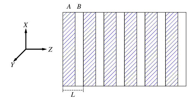
We will show that under certain physical conditions, a monochromatic plane wave incident on the semi-infinite slab is converted into an abnormal electromagnetic mode with huge amplitude and nearly tangential energy density flux, as illustrated in Fig. 3.

Such a wave will be referred to as the Axially Frozen Mode (AFM). The use of this term is justified because the normal (axial) component $u_{z}$ of the respective group velocity becomes vanishingly small, while the amplitude of the AFM can exceed the amplitude of the incident plane wave by several orders of magnitude.

The group velocity $\vec{u}$ of the AFM is parallel to the semi-infinite slab boundary and, therefore, the magnitude of the tangential component $\left(\vec{S}_{T}\right)_{\bot}$ of the respective energy density flux $\vec{S}_{T}$ is overwhelmingly larger than the magnitude of the normal component $\left(\vec{S}_{T}\right)_{z}$. But, although $\left(\vec{S}_{T}\right)_{z}\ll\left(\vec{S}_{T}\right)_{\bot}$, the normal component $\left(\vec{S}_{T}\right)_{z}$ of the energy density flux inside the slab is still comparable with that of the incident plane wave in vacuum. This property persists even if the normal component $u_{z}$ of the wave group velocity inside the slab vanishes, i.e.,

The qualitative explanation for this is that the infinitesimally small value of $u_{z}$ is offset by huge magnitude of the energy density $W$ in the AFM. As the result, the product $u_{z}W$, which determines the normal component $\left(\vec{S}_{T}\right)_{z}$ of the energy flux, remains finite. The above behavior is totally different from what happens in the vicinity of a photonic band edge, where the normal component $u_{z}$ of the wave group velocity vanishes too. Indeed, let us introduce the transmittance $\left(\tau\right)$ and the reflectance $\left(\rho\right)$ of a lossless semi-infinite slab

In line with Eq. (1), in the AFM regime the transmittance $\tau$ remains significant and can be even close to unity, as shown in an example in Fig. 4(a). In other words, the incident plane wave enters the slab with little reflectance, where it turns into an abnormal AFM with infinitesimally small normal component of the group velocity, huge amplitude, and huge tangential component of the energy density flux. By contrast, in the vicinity of a photonic band edge (at frequencies near $\omega=\omega_{b}$ in Fig. 4(a)), the transmittance of semi-infinite slab always vanishes, along with the normal component $u_{z}$ of the wave group velocity.

It turns out that at a given frequency $\omega_{0}$ the AFM regime can occur only for a special direction $\vec{n}_{0}$ of the incident plane wave propagation

This special direction of incidence always makes an oblique angle with the normal $z$ to the layers. To find $\vec{n}_{0}$ for a given $\omega_{0}$ or, conversely, to find $\omega_{0}$ for a given $\vec{n}_{0}$, one has to solve the Maxwell equations in the periodic stratified medium. This problem will be addressed in Section 3. In Section 2 we consider the relation between the AFM regime and the singularity of the electromagnetic dispersion relation responsible for such a peculiar behavior. If the frequency $\omega$ and the direction of incidence $\vec{n}$ do not match explicitly as prescribed by Eq. (3), the AFM regime will be somewhat smeared.

Let $\Psi_{T}\left(z\right)$ be the transmitted electromagnetic field inside the semi-infinite slab (the explicit definition of $\Psi_{T}\left(z\right)$ is given in Eqs. (38) and (109)). It turns out that in the vicinity of the AFM regime, $\Psi_{T}\left(z\right)$ is a superposition of the extended and evanescent Bloch eigenmodes

where $\Psi_{ex}\left(z\right)$ is an extended mode with $u_{z}>0$, and $\Psi_{ev}\left(z\right)$ is an evanescent mode with $\Im k_{z}>0$. As shown in an example in Fig. 5, both the contributions to $\Psi_{T}\left(z\right)$ have huge and nearly equal and opposite values near the slab boundary, so that their superposition (4) at $z=0$ is small enough to satisfy the boundary condition (111). As the distance $z$ from the slab boundary increases, the evanescent component $\Psi_{ev}\left(z\right)$ decays exponentially, while the amplitude of the extended component $\Psi_{ex}\left(z\right)$ remains constant and huge. As the result, the field amplitude $\left|\Psi_{T}\left(z\right)\right|^{2}$ reaches its huge saturation value $\left|\Psi_{ex}\right|^{2}$ at a certain distance from the slab boundary (see Eqs. (120), (121) and (122)).

When the direction of incidence $\vec{n}$ tends to its critical value $\vec{n}_{0}$ for a given frequency $\omega_{0}$, the respective saturation value $\left|\Psi_{ex}\right|^{2}$ of the AFM amplitude $\left|\Psi_{T}\left(z\right)\right|^{2}$ diverges as $\left|\vec{n}-\vec{n}_{0}\right|^{-2/3}$. Conversely, when the frequency $\omega$ tends to its critical value $\omega_{0}$ for a given direction of incidence $\vec{n}_{0}$, the saturation value of the AFM amplitude diverges as $\left|\omega-\omega_{0}\right|^{-2/3}$. In the real situation, of course, the AFM amplitude will be limited by such physical factors as: (i) nonlinear effects, (ii) electromagnetic losses, (iii) structural imperfections of the periodic array, (iv) finiteness of the slab dimensions, (v) deviation of the incident radiation from a perfect plane monochromatic wave.

Fig. 6 gives a good qualitative picture of what really happens in the vicinity of the AFM regime.

Consider a wide monochromatic beam of frequency $\omega$ incident on the surface of semi-infinite photonic slab. The direction of incidence $\vec{n}_{0}\parallel\vec{S}_{I}$ is chosen so that the condition (3) of the AFM regime is satisfied at $\omega=\omega_{0}$. As frequency $\omega$ tends to $\omega_{0}$ from either direction, the normal component $u_{z}$ of the transmitted wave group velocity approaches zero, while the tangential component $\vec{u}_{\perp}$ remains finite

This relation together with the equality

involving the refraction angle $\theta_{T}$, yield

Hence, in the vicinity of the AFM regime, the transmitted (refracted) electromagnetic wave can be viewed as a grazing mode. The most important and unique feature of this grazing mode directly relates to the fact that the transmittance $\tau$ of the semi-infinite slab remains finite even at $\omega=\omega_{0}$ (see, for example, Fig. 4(a)). Indeed, let $A_{I}$ and $A_{T}$ be the cross-section areas of the incident and transmitted (refracted) beams, respectively. Obliviously,

Let us also introduce the quantities

where $S_{I}$ and $S_{T}$ are the energy density fluxes of the incident and transmitted waves. $U_{I}$ and $U_{T}$ are the total power transmitted by the incident and transmitted (refracted) beams, respectively. The expressions (8) and (9) imply that

which is nothing more than a manifestation of the energy conservation law. Finally, Eq. (10), together with the formula (7), yield

where we have taken into account that $\tau S_{I}\cos\theta_{I}$ is limited (of the order of magnitude of unity) as $\omega\rightarrow\omega_{0}$. By contrast, in the vicinity of the photonic band edge the transmittance $\tau$ of the semi-infinite slab vanishes along with the energy density flux $S_{T}$ of the transmitted (refracted) wave.

The expressions (7) and (11) show that in the vicinity of the AFM regime, the transmitted wave behaves like a grazing mode with huge and nearly tangential energy density flux $S_{T}$ and very small (compared to that of the incident beam) cross-section area $A_{T}$, so that the total power $U_{T}=A_{T}S_{T}$ associated with the transmitted wave cannot exceed the total power $U_{I}$ of the incident wave: $U_{T}=\tau U_{I}\leq U_{I}$.

The above qualitative consideration is only valid on the scales exceeding the size $L$ of the unit cell (which is of the order of magnitude of $c/\omega$) and more importantly, exceeding the transitional distance $l=\left(\Im k_{ev}\right)^{-1}$ from the slab boundary where the evanescent mode contribution to the resulting electromagnetic field $\Psi_{T}\left(z\right)$ is still significant. The latter means that the width of both the incident and the refracted beams must be much larger than $l$. If the above condition is not met, we cannot treat the transmitted wave as a beam, and the expressions (7) through (11) do not apply. Instead, we would have to use the explicit electrodynamic expressions for $\Psi_{T}\left(z\right)$, such as the asymptotic formula (122). Note that if the direction $\vec{n}$ of the incident wave propagation and the frequency $\omega$ exactly match the condition (3) for the AFM regime, the transmitted wave $\Psi_{T}\left(z\right)$ does not reduce to a superposition (4) of canonical Bloch eigenmodes. Instead, the AFM is described by a general Floquet eigenmode $\Psi_{01}\left(z\right)$ from Eq. (84), which diverges inside the slab as $z$, until the nonlinear effects or other limiting factors come into play. The related mathematical analysis is provided in Sections 3 and 4.

In some respects, the remarkable behavior of the AFM, is similar to that of the frozen mode related to the phenomenon of electromagnetic unidirectionality in nonreciprocal magnetic photonic crystals PRE01; PRB03. In a unidirectional photonic crystal, electromagnetic radiation of a certain frequency $\omega_{0}$ can propagate with finite group velocity $\vec{u}\|z$ only in one of the two opposite directions, say, from right to left. The problem with the electromagnetic unidirectionality, though, is that it essentially requires the presence of magnetic materials with strong circular birefringence (Faraday rotation) and low losses at the frequency range of interest. Such materials are readily available at the microwave frequencies, but at the infrared and optical frequency ranges, finding appropriate magnetic materials is highly problematic. Thus, at frequencies above $10^{12}$ Hz, the electromagnetic unidirectionality along with the respective nonreciprocal magnetic mechanism of the frozen mode formation may prove to be impractical. By contrast, the occurrence of AFM does not require the presence of magnetic or any other essentially dispersive components in the periodic stack. Therefore, the AFM regime can be realized at any frequencies, including the infrared, optical, and even ultraviolet frequency ranges. The only essential physical requirement is the presence of anisotropic dielectric layers with proper orientation of the anisotropy axes. An example of such an array is shown in Fig. 2.

In Section 2 we establish the relation between the phenomenon of AFM and the electromagnetic dispersion relation of the periodic layered medium. This allows us to formulate strict and simple symmetry conditions for such a phenomenon to occur, as well as to find out what kind of periodic stratified media can exhibit the effect. Relevant theoretical analysis based on the Maxwell equations in stratified media is carried out in Sections 3 and 4. Finally, in Section 5 we discuss some practical aspects of the phenomenon.

First of all, notice that a periodic array would definitely have an axially symmetric dispersion relation

if the symmetry group $G$ of the periodic stratified medium includes any of the following two symmetry operations

where $m_{z}$ is the mirror plane parallel to the layers, $2_{z}$ is the 2-fold rotation about the $z$ axis, and $R$ is the time reversal operation. Indeed, since $2_{z}\left(k_{x},k_{y},k\right)=\left(-k_{x},-k_{y},k\right)$ and $R\left(k_{x},k_{y},k\right)=\left(-k_{x},-k_{y},-k\right)$, we have

which implies the relation (18) for arbitrary $\left(k_{x},k_{y}\right)$. The same is true for the mirror plane $m_{z}$

Consequently, a necessary condition for the axial spectral asymmetry (17) of a periodic stack is the absence of the symmetry operations (19), i.e.,

In reciprocal (nonmagnetic) media, where by definition, $R\in G$, instead of Eq. (20) one can use the following requirement

Note, that the axial spectral symmetry (18) is different from the bulk spectral symmetry

For example, the space inversion $I$ and/or the time reversal $R$, if present in $G$, ensure the bulk spectral symmetry (22), but neither $I$ nor $R$ ensures the axial spectral symmetry (18).

The simplest and the most practical example of a periodic stack supporting the axial spectral asymmetry (17) and, thereby, the AFM regime, is shown in Fig. 2. It is made up of anisotropic $A$ layers alternated with isotropic $B$ layers. The respective dielectric permittivity tensors are

For simplicity, we assume

The stack in Fig. 2 has the monoclinic symmetry

with the mirror plane $m_{y}$ normal to the $y$ - axis. Such a symmetry is compatible with the necessary condition (21) for the AFM existence. But as we will see below, the symmetry (28) imposes additional constraints on the direction $\vec{n}$ of the incident wave propagation.

In Fig. 9 we show the axial dispersion relation $\omega\left(k\right)$ of this periodic array, computed for four different directions $(n_{x},n_{y})$ of incident wave propagation.

These four cases cover all the possibilities, different in terms of symmetry.

In the case (a) of normal incidence, when $n_{x}=n_{y}=0$, the dispersion relation is axially symmetric, as must be the case with any reciprocal periodic stratified medium (see the explanation after Eq. (24)).

In the case (b), when $n_{x}=0$ and $n_{y}\neq 0$, the two necessary conditions (21) and (25) for the axial spectral asymmetry are met. Yet, those conditions prove not to be sufficient. Indeed, if $n_{x}=0$, either of the symmetry operations

imposes the relation

which implies the axial spectral symmetry. Neither stationary inflection point, nor AFM can occur in this case.

In the case (c), when $n_{x}\neq 0$ and $n_{y}=0$, the situation is more complicated. The quasimomentum $\vec{k}$ lies now in the $x-z$ plane, which coincides with the mirror plane $m_{y}$. Therefore, every Bloch eigenmode $\Psi_{\vec{k}}\left(z\right)$ can be classified as a pure TE or pure TM mode, depending on the $\Psi_{\vec{k}}\left(z\right)$ parity with respect to the mirror reflection $m_{y}$

The TE modes have axially symmetric dispersion relation

Indeed, the component $\varepsilon_{xz}$ of the dielectric tensor $\hat{\varepsilon}_{A}$ does not affect the TE modes, because in this case the electric component $\mathbf{E}(\mathbf{r},t)$ of the electromagnetic field is parallel to the $y$ axis. As a consequence, the axial dispersion relation of the TE spectral branches is similar to that of the isotropic case with $\varepsilon_{xz}=0$, where it is always symmetric. By contrast, for the TM modes we have $\mathbf{E}(\mathbf{r},t)\perp y$. Therefore, the TM modes are affected by $\varepsilon_{xz}$ and display axially asymmetric dispersion relation

as seen in Fig. 9(c). We wish to remark, though, that the equality (32) cannot be derived from symmetry arguments only. The axial spectral symmetry of the TE modes is not exact and relies on the approximation (27) for the magnetic permeability of the $A$ layers. On the other hand, the fact that the spectral branches have different parity (31) with respect to the symmetry operation$\ m_{y}$, implies that none of the branches can develop a stationary inflection point (see Eq. (87) and explanations thereafter). Thus, in the case $n_{y}=0$, in spite of the axial spectral asymmetry, the AFM regime cannot occur either.

Finally, in the general case (d), when $n_{x}\neq 0$ and $n_{y}\neq 0$, all the spectral branches display the property (17) of the axial spectral asymmetry. In addition, the Bloch eigenmodes now are of the same symmetry (i. e., belong to the same irreducible representation of the wave vector symmetry group) and are neither TE, nor TM. This is exactly the case when the AFM regime can be achieved at some frequencies by proper choice of the incident angle. For instance, if we impose the equality $n_{x}=$ $n_{y}$ and change the incident angle only, it turns out that every single spectral branch at some point develops a stationary inflection point (16) and, thereby, displays the AFM at the respective frequency. If we want the AFM at a specified frequency $\omega_{0}$, then we will have to adjust both $n_{x}$ and $n_{y}$.

We start with the classical Maxwell equations for time-harmonic fields in nonconducting media

where

In a lossless dielectric medium, the material tensors $\hat{\varepsilon}\left(\vec{r}\right)$ and $\hat{\mu}\left(\vec{r}\right)$ are Hermitian. In a stratified medium, the tensors $\hat{\varepsilon}\left(\vec{r}\right)$ and $\hat{\mu}\left(\vec{r}\right)$ depend on a single Cartesian coordinate $z$, and the Maxwell equations (34) can be recast as

Solutions for Eq. (36) are sought in the following form

The substitution (37) transforms the system of six linear equation (36) into a system of four linear differential equations

The explicit expression for the Maxwell operator $M\left(z\right)$ is

where

The Cartesian components of the material tensors $\hat{\varepsilon}$ and $\hat{\mu}$ are functions of $z$ and (in dispersive media) $\omega$. The reduced Maxwell equation (38) should be complemented with the following expressions for the $z$ components of the fields

where $\left(n_{x},n_{y}\right)$ are defined in Eq. (12).

Notice that in the case of normal incidence, the Maxwell operator is drastically simplified

This is the case we dealt with in PRB03 when considering the phenomenon of electromagnetic unidirectionality in nonreciprocal magnetic photonic crystals. By contrast, the objective of this Section is to show how the terms $M_{11}$ and $M_{22}$, occurring only in the case of oblique incidence, can lead to the phenomenon of AFM, regardless of whether or not the nonreciprocal effects are present. Note that $M_{11}$ and $M_{22}$ are also nonzero in materials with linear magnetoelectric effect (see, for example, Ref. 15 and references therein), but we are not considering here such an exotic situation.

Importantly, the $4\times 4$ matrix $M\left(z\right)$ in Eq. (39) has the property of $J$ - Hermitivity defined as

where

Different versions of the reduced Maxwell equation (38) can be found in the extensive literature on electrodynamics of stratified media (see, for example, Tmatrix; Abdul00; Abdul99, and references therein). For more detailed studies of $J$ - Hermitian and $J$ - unitary operators see JHerm.

The Cauchy problem

for the reduced Maxwell equation (38) has a unique solution

where the $4\times 4$ matrix $T\left(z,z_{0}\right)$ is so-called transfer matrix. From the definition (49) of the transfer matrix it follows that

The matrix $T\left(z,z_{0}\right)$ is uniquely defined by the following Cauchy problem

The equation (51), together with $J$ - Hermitivity (46) of the Maxwell operator $M\left(z\right)$, imply that the matrix $T\left(z,z_{0}\right)$ is $J$ - unitarity, i.e.,

(see the proof in Appendix 1). The $J$ - unitarity (52) of the transfer matrix imposes strong constraints on its eigenvalues (see Eq. (65)). It also implies that

The transfer matrix $T_{S}$ of a stack of layers is a sequential product of the transfer matrices $T_{m}$ of the constitutive layers

If the individual layers are homogeneous, the corresponding single-layer transfer matrices $T_{m}$ are explicitly expressed in terms of the respective Maxwell operators $M_{m}$

where $z_{m}$ is the thickness of the $m$-th layer. The explicit expression for $M_{m}$ is given by (39). Thus, formula (54), together with (55) and (39), gives us an explicit expression for the transfer matrix $T_{S}$ of an arbitrary stack of anisotropic dielectric layers. $T_{S}$ is a function of (i) the material tensors $\hat{\varepsilon}$ and $\hat{\mu}$ in each layer of the stack, (ii) the layer thicknesses, (iii) the frequency $\omega$, and (iv) the tangential components $\left(k_{x},k_{y}\right)=\left(n_{x}\omega/c,n_{y}\omega/c\right)$ of the wave vector.

Consider the important particular case of normal wave propagation. Using Eq. (55) and the explicit expression (39) for the Maxwell operator, one can prove that

Additional information related to the transfer matrix formalism can be found in Tmatrix; Abdul00; Abdul99 and references therein.

In a periodic layered structure, all material tensors, along with the $J$ - Hermitian matrix $M(z)$ in Eq. (38), are periodic functions of $z$

where $L$ is the length of a primitive cell of the periodic stack. By definition, Bloch solutions $\Psi_{k}\left(z\right)$ of the reduced Maxwell equation (38) with the periodic operator $M(z)$ satisfy

The definition (49) of the $T$ - matrix together with Eq. (58) give

Introducing the transfer matrix of a primitive cell

we have from Eq. (59)

Thus, the eigenvectors of the transfer matrix $T_{L}$ of the unit cell are uniquely related to the eigenmodes of the reduced Maxwell equation (38) through the relations

The respective four eigenvalues

of $T_{L}$ are the roots of the characteristic equation

For any given $\omega$ and $\left(k_{x},k_{y}\right)$, the characteristic equation defines a set of four values $\left\{X_{1},X_{2},X_{3},X_{4}\right\}$, or equivalently, $\left\{k_{1},k_{2},k_{3},k_{4}\right\}$. Real $k$ correspond to propagating Bloch waves (extended modes), while complex $k$ correspond to evanescent modes. Evanescent modes are relevant near photonic crystal boundaries and other structural irregularities.

The $J$-unitarity (52) of $T_{L}$ imposes the following restriction on the eigenvalues (63) for any given $\omega$ and $\left(k_{x},k_{y}\right)$

In view of the relation (65), one has to consider three different situation. The first possibility

relates to the case of all four Bloch eigenmodes being extended. The second possibility

relates to the case of two extended and two evanescent modes. The last possibility

relates the case of a frequency gap, when all four Bloch eigenmodes are evanescent.

Observe that the relation

valid in the case of normal incidence (see Refs. PRE01; PRB03), may not apply now.

The coefficients of the characteristic polynomial $F\left(X\right)$ in Eq. (64) are functions of $\omega$ and $\left(k_{x},k_{y}\right)$. Let $F_{0}\left(X\right)$ be the characteristic polynomial at the stationary inflection point (16), where $\omega=\omega_{0}$ and $\left(k_{x},k_{y}\right)=\left(k_{0x},k_{0y}\right)$. The stationary inflection point (16) can also be defined as follows

This relation requires the respective value of $X_{0}=\exp\left(ik_{0}L\right)$ to be a triple root of the characteristic polynomial $F_{0}\left(X\right)$ implying

A small deviation of the frequency $\omega$ from its critical value $\omega_{0}$ changes the coefficients of the characteristic polynomial and removes the triple degeneracy of the solution $X_{0}$

or, in terms of the axial quasimomentum $k$

References

- (1) Pochi Yeh. ”Optical Waves in Layered Media”, (Wiley, New York, 1988).
- (2) Amnon Yariv and Pochi Yeh. ”Optical waves in crystals: propagation and control of laser radiation”, (New York, Wiley, 1984).
- (3) Weng Cho Chew. ”Waves and Fields in Inhomogeneous Media”, (Van Nostrand Reinhold, New York, 1990).
- (4) Y. Fink, J. N. Winn, S. Fan, C. Chen, J. Michel, J. D. Joannopoulos, E. L. Thomas. ”A dielectric omnidirectional reflector.” Science 282 p. 1679-1682 (1998).
- (5) J. N. Winn, Y. Fink, S. Fan, J. D. Joannopoulos, ”Omnidirectional reflection from a one-dimensional photonic crystal.” Optics Letters 23, p. 1573-1575 (1998).
- (6) D. N. Chigrin, A. V. Lavrinenko, D. A. Yarotsky, S. V. Gaponenko. ”Observation of total omnidirectional reflection from a one-dimensional dielectric lattice”, Appl. Phys. A68, 25 (1999).
- (7) Ch. Luo, S. Johnson, and J. Joannopoulos. All-angle negative refraction without negative effective index. Phys. Rev. B65, 201104 (2002)
- (8) M. Notomi. Theory of light propagation in strongly modulated photonic crystals: Refractionlike behavior in the vicinity of the photonic band gap. Phys. Rev. B62, 10696 (2000)
- (9) M. Soljacic, S. Johnson, S. Fan, M. Ibanescu, E. Ippen, and J. Joannopoulos. Photonic-crystal slow-light enhancement of nonlinear phase sensitivity. J. Opt. Soc. Am. B19, 2052 (2002).
- (10) J. Bendickson, J. Dowling, and M. Scalora. Analytic expressions for the electromagnetic mode density in finite, one-dimensional, photonic band-gap structures. Phys. Rev. E53, 4107 (1996).
- (11) G. D’Aguano, M. Centini, M. Scalora, et al. Photonic band edge effects in finite structures and applications to interactions. Phys Rev. E64, 016609 (2001).
- (12) M. Scalora, R. J. Flynn, S. B. Reinhardt, and R. L. Fork, M. J. Bloemer, M. D. Tocci, C. M. Bowden, H. S. Ledbetter , J. M. Bendickson, J. P. Dowling, R. P. Leavitt. Ultrashort pulse propagation at the photonic band edge: Large tunable group delay with minimal distortion and loss. Phys. Rev. E54, R1078 (1996).
- (13) M. Scalora, M. J. Bloemer, A. S. Manka, J. P. Dowling, C. M. Bowden, R. Viswanathan, and J. W. Haus. Pulsed second-harmonic generation in nonlinear, one-dimensional, periodic structures. Phys. Rev. A56, 3166 (1997)
- (14) A. Mandatori, C. Sibilia, M. Centini, G. D’Aguanno, M. Bertolotti, M. Scalora, M. Bloemer, and C. M. Bowden. Birefringence in one-dimensional finite photonic band gap structure. J. Opt. Soc. Am. B 20, 504 (2003)
- (15) A. Figotin, and I. Vitebsky. Nonreciprocal magnetic photonic crystals. Phys. Rev. E63, 066609 (2001).
- (16) A. Figotin, and I. Vitebskiy. Electromagnetic unidirectionality in magnetic photonic crystals. Phys. Rev. B67, 165210 (2003).
- (17) D. W. Berreman. J. Opt. Soc. Am. A62, 502–10 (1972).
- (18) I. Abdulhalim. Analytic propagation matrix method for anisotropic magneto-optic layered media, J.Opt. A: Pure Appl. Opt.2, 557 (2000).
- (19) I. Abdulhalim. Analytic propagation matrix method for linear optics of arbitrary biaxial layered media, J.Opt. A: Pure Appl. Opt. 1, 646 (1999).
- (20) M. G. Krein and V. A. Jacubovich. ”Four Papers on Ordinary Differential Equations”, American Mathematical Society Translations, Series 2, Vol. 120, 1983, pp. 1-70.
- (21) R. Bellman. Introduction to Matrix Analysis. (SIAM. Philadelphia, 1997)
- (22) E. Coddington and R. Carlson. Linear Ordinary Differential Equations. (SIAM, Philadelphia, 1997).