Non-local Updates for Quantum Monte Carlo Simulations
Abstract
We review the development of update schemes for quantum lattice models simulated using world line quantum Monte Carlo algorithms. Starting from the Suzuki-Trotter mapping we discuss limitations of local update algorithms and highlight the main developments beyond Metropolis-style local updates: the development of cluster algorithms, their generalization to continuous time, the worm and directed-loop algorithms and finally a generalization of the flat histogram method of Wang and Landau to quantum systems.
1 Quantum Monte Carlo World line algorithms
Suzuki’s realization in 1976 Suzuki that the partition function of a -dimensional quantum spin- system can be mapped onto that of a -dimensional classical Ising model with special interactions enabled the straightforward simulation of arbitrary quantum lattice models, overcoming the restrictions of Handscomb’s method Handscomb. Quantum spins get mapped onto classical world lines and the Metropolis algorithm Metropolis can be employed to perform local updates of the configurations.
Just like classical algorithms the local update quantum Monte Carlo algorithm suffers from the problem of critical slowing down at second order phase transitions and the problem of tunneling out of metastable states at first order phase transitions. Here we review the development of non-local update algorithms, stepping beyond local update Metropolis schemes:
- •
1993: the loop algorithm Evertz93, a generalization of the classical cluster algorithms to quantum systems allows efficient simulations at second order phase transitions.
- •
1996: continuous time versions of the loop algorithm Beard96 and the local update algorithms Prokofev96 remove the need for an extrapolation in the discrete time step of the original algorithms (an approximation-free power-series scheme had been introduced for the S=1/2 Heisenberg model already in Handscomb, and a related, more general method with local updates was presented in Sandvik91).
- •
from 1998: the worm algorithm Prokofev98, the loop-operator Sandvik99; Dorneich and the directed loop algorithms directedloop remove the requirement of spin-inversion or particle-hole symmetry.
- •
2003: flat histogram methods for quantum systems Troyer03 allow efficient tunneling between metastable states at first order phase transitions.
2 World lines and local update algorithms
2.1 The Suzuki-Trotter decomposition
In classical simulations the Boltzmann weight of a configuration at an inverse temperature is easily calculated from its energy as . Hence the thermal average of a quantity
| (1) |
can be directly estimated in a Monte Carlo simulation. The key problem for a quantum Monte Carlo simulation is that the simple exponentials of energies get replaced by exponentials of the Hamilton operator :
| (2) |
The seminal idea of Suzuki Suzuki, using a generalization of Trotter’s formula Trotter, was to split into two or more terms so that the exponentials of each of the terms is easy to calculate. Although the do not commute, the error in estimating the exponential
| (3) |
is small for small prefactors and better formulas of arbitrarily high order can be derived Suzukihigher. Applying this approximation to the partition function we get Suzuki’s famous mapping, here shown for the simplest case of two terms and
| (4) | |||||
where the time step is , the each are complete orthonormal sets of basis states, and the transfer matrices are . The evaluation of the matrix elements is straightforward since the are chosen to be easily diagonalized.
2.2 The World Line Representation
As an example we consider a one-dimensional chain with nearest neighbor interactions. The Hamiltonian is split into odd and even bonds and , as shown in Fig. 1a). Since the bond terms in each of these sums commute, the calculation of the exponential is easy. Equation (4) can be interpreted as an evolution in imaginary time (inverse temperature) of the state by the “time evolution” operators and . Within each time interval the operators and and are each applied once. This leads to the famous “checkerboard decomposition”, a graphical representation of the sum on a square lattice, where the applications of the operators are marked by shaded squares (see Fig. 1b). The configuration along each time slice corresponds to one of the states in the sum (4).
This establishes the mapping of a one-dimensional quantum to a two-dimensional classical model where the four classical states at the corners of each plaquette interact with a four-site Ising-like interaction.

For Hamiltonians with particle number (or magnetization) conservation we can take the mapping one step further. Since the conservation law applies locally on each shaded plaquette, particles on neighboring time slices can be connected and we get a representation of the configuration in terms of world lines. The sum over all configurations with non-zero weights corresponds to the sum over all possible world line configurations. In Fig. 1b) we show such a world line configuration for a model with one type of particle (e.g. a spin-1/2, hardcore boson or spinless fermion model). For models with more types of particles there will be more kinds of world lines representing different particles (e.g. spin-up and spin-down fermions).
2.3 Local Updates
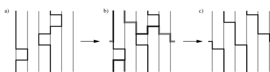
The world line representation can be used as a starting point of a quantum Monte Carlo algorithm Suzuki77. Since particle number conservation prohibits the breaking of world lines, the local updates need to move world lines instead of just changing local states as in a classical model.
As an example we consider a one-dimensional tight binding model with Hamiltonian
| (5) |
where creates a particle (spinless fermion or hardcore boson) at site . Fig. 2a shows the plaquette weights for each of the six world line configurations on a shaded plaquette in this model.
The local updates are quite simple and move a world line across a white plaquette Suzuki77; Hirsch, as shown in Fig. 2b). Slightly more complicated local moves are needed for higher-dimensional models Makivic92, - models Assaad; Troyer94 and Kondo lattice models Troyer94.
Since these local updates cannot change global properties, such as the number of world lines or their spatial winding, they need to be complemented with global updates if the grandcanonical ensemble should be simulated Makivic92. The problem of exponentially low acceptance rate of such moves was remedied only much later by the non-local update algorithms discussed below.

2.4 The Continuous Time Limit
The systematic error arising from the finite time step was originally controlled by an extrapolation to the continuous time limit from simulations with different values of the time step . It required a fresh look at quantum Monte Carlo algorithms by a Russian group Prokofev96 in 1996 to realize that, for a discrete quantum lattice model, this limit can already be taken during the construction of the algorithm and simulations can be performed directly at , corresponding to an infinite Trotter number .
In this limit the Suzuki-Trotter formula Eq. (4) becomes equivalent to a time-dependent perturbation theory in imaginary time Prokofev96; Prokofev98:
| (6) | |||||
where the symbol denotes time-ordering of the exponential. The Hamiltonian is split into a diagonal term and an offdiagonal perturbation . The time-dependent perturbation in the interaction representation is . In the case of the tight-binding model the hopping term is part of the perturbation , while additional diagonal potential or interaction terms would be a part of .
To implement a continuous time algorithm the first change in the algorithm is to keep only a list of times at which the configuration changes instead of storing the configuration at each of the time slices in the limit . Since the probability for a jump of a world line [see Fig. 2a)] and hence a change of the local configuration is the number of such changes remains finite in the limit . The representation is thus well defined, and, equivalently, in Eq. (6) only a finite number of terms contributes in a finite system.
The second change concerns the updates, since the probability for the insertion of a pair of jumps in the world line [the upper move in Fig. 2b)] vanishes as
| (7) |
in the continuous time limit. To counter this vanishing probability, one proposes to insert a pair of jumps not at a specific location but anywhere inside a finite time interval Prokofev96. The integrated probability then remains finite in the limit . Similarly instead of shifting a jump by [the lower move in Figs. 2b,c)] we move it by a finite time interval in the continuous time algorithm.
2.5 Stochastic Series Expansion
An alternative Monte Carlo algorithm, which also does not suffer from time discretization, is the stochastic series expansion (SSE) algorithm Sandvik91, a generalization of Handscomb’s algorithm Handscomb for the Heisenberg model. It starts from a Taylor expansion of the partition function in orders of :
| (8) | |||||
where in the second line we decomposed the Hamiltonian into a sum of single-bond terms , and again inserted complete sets of basis states. We end up with a similar representation as Eq. (4) and a related world-line picture with very similar update schemes. For more details of the SSE method we refer to the contribution of A.W. Sandvik in this proceedings volume.

The SSE representation can be formally related to the world line representation by observing that Eq. (8) is obtained from Eq. (6) by setting , and integrating over all times (compare also Fig. 3) Sandvik97. This mapping also shows the advantages and disadvantages of the two representations. The SSE representation corresponds to a perturbation expansion in all terms of the Hamiltonian, whereas world line algorithms treat the diagonal terms in exactly and perturb only in the offdiagonal terms of the Hamiltonian. World line algorithms hence need only fewer terms in the expansion, but pay for it by having to deal with imaginary times . The SSE representation is thus preferred except for models with large diagonal terms (e.g. bosonic Hubbard models) or for models with time-dependent actions (e.g. dissipative quantum systems CaldeiraLegget).
3 The loop algorithm
While the local update world line and SSE algorithms enable the simulation of quantum systems they suffer from critical slowing down at second order phase transitions. Even worse, changing the spatial and temporal winding numbers has an exponentially small acceptance rate. While the restriction to zero spatial winding can be viewed as a boundary effect, changing the temporal winding number and thus the magnetization or particle number is essential for simulations in the grand canonical ensemble.
The solution to these problems came with the loop algorithm Evertz93 and its continuous time version Beard96. These algorithms, generalizations of the classical cluster algorithms SwendsenWang to quantum systems, not only solve the problem of critical slowing down, but also updates the winding numbers efficiently for those systems to which it can be applied.

Since there is an extensive recent review of the loop algorithm Evertz03, we will only mention the main idea behind the loop algorithm here. In the classical Swendsen-Wang cluster algorithm each bond in the lattice is considered, and with a probability depending on the local configuration two neighboring spins are either “connected” or left “disconnected”, as shown in Fig. 4a). “Connected” spins form a cluster and must be flipped together. Since the average extent of these cluster is just the correlation length of the system, updates are performed on physically relevant length scales and autocorrelation times are substantially reduced.
Upon applying the same idea to world lines in QMC we have to take into account that (in systems with particle number or magnetization conservation) the world lines may not be broken. This implies that a single spin on a plaquette cannot be flipped by itself, but at least two, or all four spins must be flipped in order to create valid updates of the world line configurations. Instead of the two possibilities “connected” or “disconnected”, four connections are possible on a plaquette, as shown in Fig. 4b): either horizontal neighbors, vertical neighbors, diagonal neighbors or all four spins might be flipped together. The specific choices and probabilities depend, like in the classical algorithm, on details of the model and the world line configuration. Since each spin is connected to two (or four) other spins, the cluster has a loop-like shape (or a set of connected loops), which is the origin of the name “loop algorithm” and is illustrated in Fig. 5.
While the loop algorithm was originally developed only for six-vertex and spin-1/2 models Evertz93 it has been generalized to higher spin models higherspin, anisotropic spin models anisotropicspin, Hubbard hubbard and - models Ammon.
3.1 Applications of the loop algorithm
Out of the large number of applications of the loop algorithm we want to mention only a few which highlight the advances made possible by the development of this algorithm and refer to Ref. Evertz03 for a more complete overview.
- •
- •
The exponential divergence of the correlation length in the same system could be studied on much larger systems with up to one million spins Kim97; Kim98; Beard98 and with much higher accuracy than in previous simulations Makivic92, investigating not only the leading exponential behavior but also higher order corrections.
- •
For quantum phase transitions in two-dimensional quantum Heisenberg antiferromagnets, simulations using local updates had been restricted to small systems with up to 200 spins at not too low temperatures and had given contradicting results regarding the universality class of the phase transitions Sandvik94; Katoh94. The loop algorithm enabled simulations on up to one hundred times larger systems at ten times lower temperatures, allowing the accurate determination of the critical behavior at quantum phase transitions Troyer97; Sandvik00.
- •
Similarly, in the two-dimensional quantum model the loop algorithm allowed accurate simulations of the Kosterlitz-Thouless phase transition Harada97, again improving on results obtained using local updates Makivic92b.
- •
- •
A generalization, which allows to study infinite systems in the absence of long range order, was invented Evertz01.
- •
The meron cluster algorithm, an algorithm based on the loop algorithm, solves the negative sign problem in some special systems Wiese99.
4 Worm and directed loop algorithms
4.1 Problems of the loop algorithm in a magnetic field
As successful as the loop algorithm is, it is restricted – as the classical cluster algorithms – to models with spin inversion symmetry (or particle-hole symmetry). Terms in the Hamiltonian which break this spin-inversion symmetry – such as a magnetic field in a spin model or a chemical potential in a particle model – are not taken into account during loop construction. Instead they enter through the acceptance rate of the loop flip, which can be exponentially small at low temperatures.

As an example consider two quantum spins in a magnetic field:
| (9) |
In a field the singlet state with energy is degenerate with the triplet state with energy , but he loop algorithm is exponentially inefficient at low temperatures. As illustrated in Fig. 6a), we start from the triplet state and propose a loop shown in Fig. 6b). The loop construction rules, which do not take into account the magnetic field, propose to flip one of the spins and go to the intermediate configuration with energy shown in Fig. 6c). This move costs potential energy and thus has an exponentially small acceptance rate . Once we accept this move, immediately many small loops are built, exchanging the spins on the two sites, and gaining exchange energy by going to the spin singlet state. A typical world line configuration for the singlet is shown in Fig. 6d). The reverse move has the same exponentially small probability, since the probability to reach a world line configuration without any exchange term [Fig. 6c)] from a spin singlet configuration [Fig. 6d)] is exponentially small.
This example clearly illustrates the reason for the exponential slowdown: in a first step we lose all potential energy, before gaining it back in exchange energy. A faster algorithm could thus be built if, instead of doing the trade in one big step, we could trade potential with exchange energy in small pieces, which is exactly what the worm algorithm does.
4.2 The Worm Algorithm
The worm algorithm Prokofev98 works in an extended configuration space, where in addition to closed world line configurations one open world line fragment (the “worm”) is allowed. Formally this is done by adding a source term to the Hamiltonian which for a spin model is
| (10) |
This source term allows world lines to be broken with a matrix element proportional to . The worm algorithm now proceeds as follows: a worm (i.e. a world line fragment) is created by inserting a pair of operators at nearby times, as shown in Fig. 7a,b). The ends of this worm are then moved randomly in space and time [Fig. 7c)], using local Metropolis or heat bath updates until the two ends of the worm meet again as in Fig. 7d). Then an update which removes the worm is proposed, and if accepted we are back in a configuration with closed world lines only, as shown in Fig. 7e). This algorithm is straightforward, consisting just of local updates of the worm ends in the extended configuration space but it can perform nonlocal changes. A worm end can wind around the lattice in the temporal or spatial direction and that way change the magnetization and winding number.

In contrast to the loop algorithm in a magnetic field, where the trade between potential and exchange energy is done by first losing all of the potential energy, before gaining back the exchange energy, the worm algorithm performs this trade in small pieces, never suffering from an exponentially small acceptance probability. While not being as efficient as the loop algorithm in zero magnetic field (the worm movement follows a random walk while the loop algorithm can be interpreted as a self-avoiding random walk), the big advantage of the worm algorithm is that it remains efficient in the presence of a magnetic field.
A similar algorithm was already proposed more than a decade earlier Cullen83. Instead of a random walk using fulfilling detailed balance at every move of the worm head in this earlier algorithm just performed a random walk. The a posteriori acceptance rates are then often very small and the algorithm is not efficient, just as the small acceptance rates for loop updates in magnetic fields make the loop algorithm inefficient. This highlights the importance of having the cluster-building rules of a non-local update algorithm closely tied to the physics of the problem.
4.3 The Directed Loop Algorithm
Algorithms with a similar basic idea are the operator-loop update Sandvik99; Dorneich in the SSE formulation and the directed-loop algorithms directedloop which can be formulated in both an SSE and a world-line representation. Like the worm algorithm, these algorithms create two world line discontinuities, and move them around by local updates. The main difference to the worm algorithm is that here these movements do not follow an unbiased random walk but have a preferred direction, always trying to move away from the last change. The directed loop algorithms might thus be more efficient than the worm algorithm but no direct comparison has been performed so far. For more details see the contribution of A.W. Sandvik in this volume.
4.4 Applications
Just as the loop algorithm enabled a break-through in the simulation of quantum magnets in zero magnetic field, the worm and directed loop algorithms allowed simulations of bosonic systems with better efficiency and accuracy. A few examples include:
- •
Simulations of quantum phase transitions in soft-core bosonic systems, both for uniform models Prokofev98 and in magnetic traps Prokofev02.
- •
By being able to simulate substantially larger latttices than by local updates Batrouni the existence of supersolids in hard-core boson models was clarified Hebert01 and the ground-state Hebert01; Bernardet02 and finite-temperature phase diagrams Schmid of two-dimensional hard-core boson models have been determined.
- •
Magnetization curves of quantum magnets have been calculated Kashurnikov99.
5 Flat Histograms and First Order Phase Transitions
The main problem during the simulation of a first order phase transition is the exponentially slow tunneling time between the two coexisting phases. For classical simulations the multi-canonical algorithm Berg92 and recently the Wang-Landau algorithm WangLandau eases this tunneling by reweighting configurations such as to achieve a “flat histogram” in energy space. In a canonical simulation the probability of visiting an energy level is where the density of states is the number of states with energy . While the multi-canonical algorithm Berg92 changes the canonical distribution by reweighting it in an energy-dependent way, the algorithm by Wang and Landau discards the notion of temperature and directly uses the density of states to set , which gives a constant probability in energy space . The unknown quantity is determined self-consistently in an iterative way and then allows to directly calculate the free energy
| (11) |
and other thermodynamic quantities at any temperature. The main change to a simulation program using a canonical distribution is to replace the canonical probability by the inverse density of states .
This algorithm cannot be straightforwardly used for quantum systems, since the density of states is not directly accessible for those. Instead we recently proposed Troyer03 to start from the SSE formulation of the partition function Eq. (8):
| (12) | |||||
The coefficient of the -th order term in an expansion in the inverse temperature now plays the role of the density of states in the classical algorithm. Similar to the classical algorithm, by using as the probability of a configuration instead of the usual SSE weight, a flat histogram in the order of the series is achieved. Alternatively instead of such a high-temperature expansion a finite-temperature perturbation series can be formulated Troyer03.
This algorithm was shown to be effective at first order phase transitions in quantum systems and promises to be effective also for the simulation of quantum spin glasses.
6 Which algorithm is the best?
Since there is no “best algorithm” suitable for all problems we conclude with a guide on how to pick the best algorithm for a particular problem.
- •
For models with particle-hole or spin-inversion symmetry a loop algorithm is optimal Evertz93; Beard96; Sandvik99. Usually an SSE representation Sandvik99 will be preferred unless the action is time-dependent (such as long-range in time interactions in a dissipative quantum system) or there are large diagonal terms, in which case a world line representation is better.
- •
For models without particle hole symmetry a worm or directed-loop algorithm is the best choice:
- –
if the Hamiltonian is diagonally dominant use a worm Prokofev98 or directed loop directedloop algorithm in a world line representation.
- –
otherwise ause directed-loop algorithm in an SSE representation. Sandvik99; Dorneich; directedloop.
- –
- •
At first order phase transition a generalization of Wang-Landau sampling to quantum systems should be used Troyer03.
The source code for some of these algorithms is available on the Internet. Sandvik has published a FORTRAN version of an SSE algorithm for quantum magnets SandvikCode. The ALPS (Algorithms and Libaries for Physics Simulations) project is an open-source effort to provide libraries and application frameworks for classical and quantum lattice models as well as C++ implementations of the loop, worm and directed-loop algorithms ALPS.
References
- (1) M. Suzuki, Prog. of Theor. Phys. 56, 1454 (1976).
- (2) D.C. Handscomb, Proc. Cambridge Philos. Soc. 58, 594 (1962).
- (3) N. Metropolis, A. R. Rosenbluth, M. N. Rosenbluth, A. H. Teller and E. Teller, J. of Chem. Phys. 21, 1087 (1953).
- (4) H.G. Evertz, G. Lana and M. Marcu, Phys. Rev. Lett. 70, 875 (1993).
- (5) B.B. Beard and U.-J. Wiese, Phys. Rev. Lett. 77, 5130 (1996).
- (6) N.V. Prokof’ev, B.V. Svistunov and I.S. Tupitsyn, Pis’ma v Zh.Eks. Teor. Fiz., 64, 853 (1996) [English translation is Report cond-mat/9612091].
- (7) A.W. Sandvik and J. Kurkijärvi, Phys. Rev. B 43, 5950 (1991).
- (8) N.V. Prokof’ev, B.V. Svistunov and I.S. Tupitsyn, Sov. Phys. - JETP 87, 310 (1998).
- (9) A.W. Sandvik, Phys. Rev. B 59, R14157 (1999).
- (10) A. Dorneich and M. Troyer, Phys. Rev. E 64, 066701 (2001).
- (11) O.F. Syljuåsen and A.W. Sandvik, Phys. Rev. E 66, 046701 (2002); O.F. Syljuåsen, Phys. Rev. E 67, 046701 (2003).
- (12) M. Troyer, S. Wessel and F. Alet, Phys. Rev. Lett. 90, 120201 (2003).
- (13) H.F. Trotter, Proc. Am. Math. Soc. 10, 545 (1959).
- (14) M. Suzuki, Phys. Lett. A 165, 387 (1992).
- (15) M. Suzuki, S. Miyashita and A. Kuroda, Prog. Theor. Phys. 58, 1377 (1977).
- (16) J.E. Hirsch, D.J. Scalapino, R.L. Sugar and R. Blankenbecler, Phys. Rev. Lett. 47, 1628 (1981).
- (17) M.S. Makivić and H.-Q. Ding, Phys. Rev. B 43, 3562 (1991).
- (18) F.F. Assaad and D. Würtz, Phys. Rev. B 44, 2681 (1991).
- (19) M. Troyer, Ph.D. thesis (ETH Zürich, 1994).
- (20) A. W. Sandvik, R. R. P. Singh and D. K. Campbell, Phys. Rev. B 56, 14510 (1997).
- (21) A.O. Caldeira and A.J. Leggett, Phys. Rev. Lett. 46, 211 (1981).
- (22) R.H. Swendsen and J.-S. Wang, Phys. Rev. Lett. 58, 86 (1987).
- (23) H.G. Evertz, Adv. Phys. 52, 1 (2003).
- (24) N. Kawashima and J. Gubernatis, J. Stat. Phys. 80, 169 (1995); K. Harada, M. Troyer and N. Kawashima, J. Phys. Soc. Jpn. 67, 1130 (1998); S. Todo and K. Kato , Phys. Rev. Lett. 87, 047203 (2001).
- (25) N. Kawashima, J. Stat. Phys. 82, 131 (1996).
- (26) N. Kawashima, J. E. Gubernatis and H. G. Evertz, Phys. Rev. B 50, 136 (1994).
- (27) B. Ammon, H.G. Evertz, N. Kawashima, M. Troyer and B. Frischmuth, Phys. Rev. B 58, 4304 (1998).
- (28) U.-J. Wiese and H.-P. Ying, Z. Phys. B 93, 147 (1994).
- (29) J.-K. Kim, D.P. Landau and M. Troyer, Phys. Rev. Lett. 79, 1583 (1997).
- (30) J.-K. Kim and M. Troyer, Phys. Rev. Lett. 80, 2705 (1998).
- (31) B.B. Beard, R.J. Birgeneau, M. Greven and U.-J. Wiese, Phys. Rev. Lett. 80, 1742 (1998).
- (32) A.W. Sandvik and D.J. Scalapino, Phys. Rev. Lett. 72, 2777 (1994).
- (33) N. Katoh and M. Imada, J. Phys. Soc. Jpn. 63, 4529 (1994).
- (34) M. Troyer, M. Imada and K. Ueda, J. Phys. Soc. Jpn. 66, 2957 (1997).
- (35) P.V. Shevchenko, A.W. Sandvik and O.P. Sushkov Phys. Rev. B 61, 3475 (2000).
- (36) K. Harada and N. Kawashima, Phys. Rev. B 55, R11949 (1997).
- (37) M.S. Makivić, Phys. Rev. B 46, 3167 (1992).
- (38) G. Santoro, S. Sorella, L. Guidoni, A. Parola and E. Tosatti Phys. Rev. Lett. 83, 3065 (1999)
- (39) K. Harada, N. Kawashima and M. Troyer, Phys. Rev. Lett. 90, 117203 (2003).
- (40) H.G. Evertz and W. von der Linden, Phys. Rev. Lett. 86, 5164 (2001).
- (41) S. Chandrasekharan and U.-J. Wiese, Phys. Rev. Lett. 83, 3116 (1999).
- (42) J.J. Cullen and D.P. Landau, Phys. Rev. B 27, 297 (1983).
- (43) V. A. Kashurnikov, N. V. Prokof’ev and B. V. Svistunov Phys. Rev. A 66, 031601 (2002).
- (44) G.G. Batrouni, R.T. Scalettar, A.P. Kampf and G.T. Zimanyi, Phys. Rev. Lett. 74, 2527 (1995), R.T. Scalettar, G.G. Batrouni, A.P. Kampf and G.T. Zimanyi, Phys. Rev. B 51, 8467 (1995); G.G. Batrouni and R.T. Scalettar, Phys. Rev. Lett. 84, 1599 (2000).
- (45) F. Hebert, G.G. Batrouni, R.T. Scalettar, G. Schmid, M. Troyer and A. Dorneich, Phys. Rev. B 65, 014513 (2001).
- (46) K. Bernardet, G.G. Batrouni, J.-L. Meunier, G. Schmid, M. Troyer and A. Dorneich, Phys. Rev. B 65, 104519 (2002).
- (47) G. Schmid, S. Todo, M. Troyer and A. Dorneich, Phys. Rev. Lett. 88, 167208 (2002); G. Schmid and M. Troyer, Report cond-mat/0304657.
- (48) V.A. Kashurnikov, N.V. Prokof’ev, B.V. Svistunov and M. Troyer, Phys. Rev. B 59, 1162 (1999).
- (49) B.A. Berg and T. Neuhaus, Phys. Lett. B. 267, 249 (1991); Phys. Rev. Lett. 68, 9 (1992).
- (50) F. Wang and D. P. Landau, Phys. Rev. Lett. 86, 2050 (2001); Phys. Rev. E 64, 056101 (2001).
- (51) http://www.abo.fi/~physcomp/
- (52) Codes will be available from http://alps.comp-phys.org/ by the end of 2003, before this article will be published.