Exo-interferometric Phase Determination of X rays
Abstract
The time-dependent phase change of x rays after transmission through a sample has been determined experimentally. We used an x-ray interferometer with a reference sample containing sharp nuclear resonances to prepare a phase-controlled x-ray beam. A sample with similar resonances was placed in the beam but outside of the interferometer; hence our use of the term “exo-interferometric.” We show that the phase change of the x rays due to the sample can be uniquely determined from the time-dependent transmitted intensities. The energy response of the sample was reconstructed from the phase and the intensity data with a resolution of 23 neV.
pacs
42.87.Bg, 42.25.Hz, 76.80.+y, 78.70.CkParticle scattering, particularly of photons, is one of the most widely used tools in science. The measured quantity is usually the particle flux or the intensity. The phase of the particle field, or more precisely the phase change of the field during the scattering process, goes undetected by the intensity measurement. The related loss of information is known as the “phase problem” in various areas of research.
Methods of phase determination are commonly based on creating two or more indistinguishable paths for the particle where at least one path does not include the sample. The resulting interference pattern is then accessible by intensity measurements. Interferometric techniques with x rays Bonse65; Bonse77; Hirano96, light HariharanMalacara, neutrons RauchWerner, or atoms Berman have been developed in this context. Results usually depend on details in the detected interference pattern, and measurements become exceedingly difficult for short wavelengths. In the x-ray regime, thermal and mechanical stability of the interferometer (IFM) are crucial, and the spatial limitations on a sample in close proximity to sensitive components of the IFM can be problematic for experimental work. Here we discuss an x-ray interferometric method that avoids this problem.
The typical x-ray IFM works with sample and reference placed in spatially separate paths inside the IFM. This allows the comparison of phase changes to the photon field caused by sample and reference. Besides potential stability problems, interference is not achieved if the direction of the x rays is changed by a scattering process in the sample. The spatial separation of x-ray IFM and sample for phase measurements would be highly desirable but to our knowledge has not been demonstrated previously. In this paper, we present measurements of phase changes caused by a sample placed outside the IFM, i.e., after recombination of the beam paths. We use the term “exo-interferometry” to emphasize this fact. Exo-interferometry permits us to analyze phase changes of x rays that were transmitted, reflected, or diffracted by a sample material. Our approach is based on recent theoretical work Sturhahn01 on time-dependent phase determination using an x-ray IFM. For experimental verification, we used a coherent nuclear resonant scattering process GerdauDeWaard, which produces a signal that is sufficiently delayed to be observable by x-ray detectors. Previous experiments on nuclear resonant interferometry Hasegawa94; Izumi95 placed samples inside the IFM and did not attempt to obtain the time-dependent phase. The principles of exo-interferometric phase determination are elucidated next.
The addition of field amplitudes in the IFM allows the production of a time-dependent field with a phase that can be manipulated in a controlled way. Consider a very short x-ray pulse described by that is incident on a triple-Laue IFM similar to the schematic shown in Fig. 1. If we place a reference material with response function in one of the paths of the IFM and apply an additional phase shift between the two paths, the exit field will be roughly proportional to . It will be useful to introduce the delayed response explicitly. Let , where is the delayed response that vanishes for “early” times after arrival of the x-ray pulse. The field amplitude after the IFM is then given by
| (1) |
At early times, modulus and phase of the field are controlled by the phase shift , whereas at later times the components of the field are unaffected. The basic idea of exo-interferometric phase determination is now to mix field components with different time coordinates simply by scattering the x-ray field described by Eq. (1) off a sample. The degree of mixing will depend on the properties of the sample and on the adjustable value of . If the response of the sample material is prompt, i.e., proportional to , mixing does not occur – a delayed response is required. Assume the transmission through a sample with response function with delayed part . The expression for the field amplitude after the sample contains three terms
| (2) |
The first term describes conventional x-ray interferometry. The second term is reminiscent of the coherent superposition of delayed reference and sample response that is observed when placing the sample inside the IFM. The last term is a convolution integral that also gives a delayed contribution. A similar expression, but all terms with being absent, has been used to describe “time-domain interferometry” Baron97; Smirnov01.
The previous arguments lead to the following conclusions about the feasibility of exo-interferometric experiments. Reference and sample must produce time-delayed responses, and the convolution of the responses should be negligible, i.e., either the spectra of and have a small overlap or the response is sufficiently weak. There must be a time scale that clearly separates “early” and “delayed.” However, the time scale does not enter quantitatively – it is mostly determined by experimental circumstances. The response time of an x-ray IFM using single crystals with low-order Bragg or Laue reflections is of the order 10-15 s. In the present experiment, the x-ray pulses incident on the IFM had a longitudinal coherence time of about 0.3 ps corresponding to an energy bandwidth of 2 meV. In addition, the average length of the synchrotron radiation (SR) pulse, 70 ps, and the time resolution of the x-ray detector, 1 ns, have to be considered. Mainly caused by detector resolution, the time scale is placed in the nanosecond regime. The time scale for the nuclear-resonant response of sample and reference is determined by the lifetime of the nuclear excited state, which is 141 ns for the 14.4125 keV nuclear level of the 57Fe isotope used here.

Experiments were performed at sector 3 of the Advanced Photon Source. The storage ring was filled with 23 electron bunches producing about 6.2106 x-ray pulses per second. The SR was monochromatized to about 2 meV bandwidth to avoid overload of the detector system while maintaining the spectral brightness of the x rays around the nuclear transition energy. After reduction of the beam size to 0.30.3 mm2, the photon flux was 109 ph/s and about 3107 ph/s after the triple-Laue IFM. A schematic of the experimental setup is shown in Fig. 1. Three situations were realized : the sample is placed outside the IFM and magnetized collinear with the linear polarization of the SR, as before but magnetized perpendicular to polarization and propagation direction of the SR, the sample is mounted inside the IFM and magnetized parallel to the polarization direction of the SR. In all cases, the reference was a 1.1-m-thick foil of stainless steel (Fe0.55Cr0.25Ni0.2) that was 95 % enriched in the 57Fe isotope. The sample outside the IFM was a 2.5-m-thick iron foil that was 53 % enriched in the 57Fe isotope. The control measurements with sample inside the IFM used a 2.2-m-thick iron foil that was 95 % enriched in the 57Fe isotope. Very good knowledge of the time response of magnetized iron and stainless steel motivated this choice.

For each experimental situation, we measured six time spectra : the phase retarder adjusted to , and either IFM path blocked. The spectra were collected in back-to-back sequences of 10 min/spectrum to minimize systematical errors caused by potential beam instabilities and temperature drifts.
Temperature variations during the experiment were less than 150 mK. For the control case, the relative phase change of the x-rays by the sample is calculated from the four interference spectra without specific knowledge about the IFM imperfections. With and , we obtain from ref. Sturhahn01 for the time-dependent phase angle
| (3) |
The time spectra for the different phase-retarder settings, the time spectrum of the sample alone, and the derived phase angle, , are shown in Fig. 2. A standard evaluation code, Conuss Sturhahn00, was used to fit the spectrum of the sample. The excellent agreement supports the notion of well-defined hyperfine interaction parameters of the chosen iron foil.

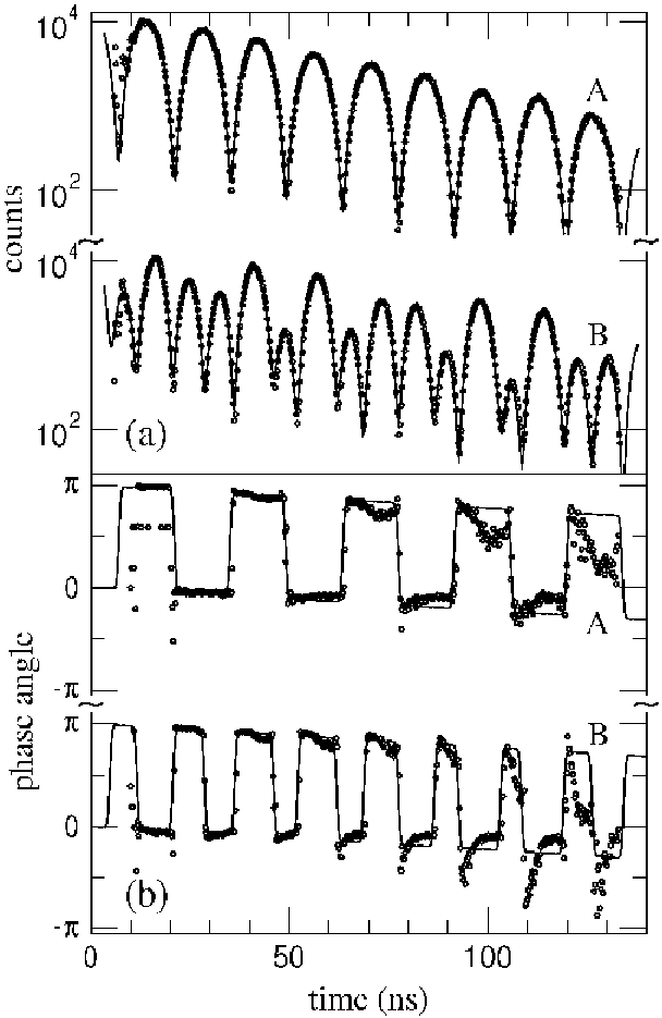
If the sample is placed outside the IFM, Eq. (2) is applied, and, if one neglects the convolution integral, the relative phase results from Eq. (3) with the replacement . The last term is composed of the time spectrum of the sample, , and a factor that accounts for absorption in the reference and IFM imperfections. is the product of IFM visibility, 0.45 in this case, and intensity ratio of the individual IFM paths. We determined experimentally . Fig. 3 shows the time-dependent intensities and phases for the two directions of magnetization with the sample outside the IFM. In Figs. 2 and 3, one notices overshoots at phase jumps, i.e., at sign changes of the transmitted electric field associated with zero intensity. In those minima, the measurement is most sensitive to effects of the detector resolution and potentially other systematic errors. However, the resulting phase errors are associated with very small field amplitudes, which reduces their significance.
The determination of the time-dependent phase as described in the previous section did not require specific knowledge of reference or sample. The phase angle together with the measured intensities of the sample alone, as displayed in Figs. 2 and 3, permits us to reconstruct the energy response of the sample by Fourier transformation
| (4) |
In this expression, is the time spectrum of the sample, shown in Figs. 2(b) and 3(a), and is the phase angle determined earlier and shown in Figs. 2(c) and 3(b). was calculated for each sequence of data (about 1h collection time). In Fig. 4, we show the reconstructed energy spectra for each data sequence, the average of all data sequences, and the calculated energy spectra. The oscillation pattern in the time spectra and the separation of the resonances in the energy spectra are dominated by the magnetic field at the 57Fe nuclei. The results for magnetic field values agree within 0.03 % for the control case and within 0.2 % and 0.7 % for the exo-interferometric situations A and B. In addition, the reconstructed energy spectra contain a small but noticeable overall shift, the so-called isomeric shift. One obtains 1.037(6) for the control case, in agreement with the literature value of 0.9(2) MBdataIx74. The exo-interferometric situations A and B give 1.05(2) and 0.67(2) for the same quantity. The values are given in units of =4.66 neV, the width of the nuclear-excited state. In our measurement, we used an avalanche photodiode detector with about 1 ns resolution, which results in an accessible energy range in the reconstructed spectrum of about 140 =0.66 eV. The energy resolution is related to the observed duration of the time-delayed signal Sturhahn01. Here the time duration of 116 ns was determined by the operating mode of the Advanced Photon Source and detector dead time. It leads to an energy resolution of 23 neV. The additional broadening of the resonances in Fig. 4 is caused by thickness-related self-absorption effects in the samples. The agreement of calculation and reconstructed spectra is generally very good even though Fig. 4 shows deviations, which appear to be stronger for the exo-interferometric cases. Also for the control case, a slight asymmetry in the spectrum can be observed. Possible explanations include inhomogeneity in sample or reference and non random imperfections of the IFM. At present, we have no conclusive explanation for these small but noticeable effects. In situation B, our neglect of the convolution term in Eq. (2), which amounts to an approximation in the process of phase determination, leads to larger deviations of, e.g., the measured isomeric shift. A glance at Fig. 4 B shows that two resonances of the sample are rather close to the origin of the energy scale, which marks the position of the single resonance of the stainless-steel reference. The overlap of the energy spectra leads to a stronger contribution of the convolution term than in situation A, and its neglect causes a larger distortion in the reconstructed energy spectra.
Exo-interferometry has been introduced as spectroscopic use of an x-ray IFM with distinct advantages in sample utilization. The ideas of exo-interferometry are general, but potential applications need to use technically available time scales, which are essentially given by the best time resolution of x-ray detectors. At present, streak cameras provide ps resolution, which could make a meV-energy range accessible with eV resolution. The presented data have unambigously demonstrated that time-dependent phase changes in x-ray fields can be measured with samples positioned inside or outside an x-ray IFM. To demonstrate the principle, our studies were conducted in transmission geometry. But, in contrast to conventional x-ray interferometry, crystal diffraction or surface reflection could be investigated as well. For example, in pump-probe time-resolved x-ray diffraction experiments Reis01, exo-interferometric phase determination may become a very useful tool. It also becomes possible to manipulate the x-ray beam between IFM and sample, e.g., by focusing or polarization control.
We want to thank J. Zhao for valuable support during beamline operations. This work was supported by the U.S. Department of Energy, Basic Energy Sciences, Office of Science, under Contract No. W-31-109-Eng-38.
References
- (1) U. Bonse and M. Hart, Appl.Phys.Lett. 6, 155 (1965); 7, 99 (1965); Z.Physik 188, 154 (1965)
- (2) U. Bonse and W. Graeff, in X-ray Optics edited by H.-J. Queisser (Springer-Verlag, Berlin, 1977), pp.93-143
- (3) K. Hirano, A. Momose, Phys.Rev.Lett. 76, 3735 (1996)
- (4) P. Hariharan and D. Malacara, Selected Papers on Interference, Interferometry, and Interferometric Metrology (SPIE Optical Engineering Press, Bellingham, WA, 1995)
- (5) H. Rauch and S.A. Werner, Neutron Interferometry : Lessons in Experimental Quantum Mechanics (Oxford University Press, New York, 2000)
- (6) P.R. Berman, Atom Interferometry (Academic Press, San Diego, CA, 1997)
- (7) W. Sturhahn, Phys.Rev. B 63, 094105 (2001)
- (8) E. Gerdau and H. de Waard, eds., Nuclear Resonant Scattering of Synchrotron Radiation, Hyperfine Int. 123-125, (1999/2000)
- (9) Y. Hasegawa et al., Phys.Rev. B 50, 17748 (1994)
- (10) K. Izumi et al., Jpn. J. Appl. Phys. 34, 4258 (1995)
- (11) A.Q.R. Baron et al., Phys.Rev.Lett. 79, 2823 (1997)
- (12) G.V. Smirnov, V.G. Kohn, W. Petry, Phys.Rev. B 63, 144303 (2001)
- (13) W. Sturhahn, Hyperfine Int. 125, 149 (2000); W. Sturhahn and E. Gerdau, Phys.Rev. B 49, 9285 (1994)
- (14) J. Stevens, ed., Mössbauer Data Index (Plenum Press, New York, 1974)
- (15) D.A. Reis et al., Phys.Rev.Lett. 86, 3072 (2001)