DEFLECTIONS IN MAGNET FRINGE FIELDS
Abstract
A transverse multipole expansion is derived, including the longitudinal components necessarily present in regions of varying magnetic field profile. It can be used for exact numerical orbit following through the fringe field regions of magnets whose end designs introduce no extraneous components, i.e. fields not required to be present by Maxwell’s equations. Analytic evaluations of the deflections are obtained in various approximations. Mainly emphasized is a “straight-line approximation”, in which particle orbits are treated as straight lines through the fringe field regions. This approximation leads to a readily-evaluated figure of merit, the ratio of r.m.s. end deflection to nominal body deflection, that can be used to determine whether or not a fringe field can be neglected. Deflections in “critical” cases (e.g. near intersection regions) are analysed in the same approximation.
pacs
PACS numbers:I STRATEGY AND NOTATION
The purpose of this paper is to derive formulas for the orbit deflections caused by the fringe fields of non-solenoidal accelerator magnets. The main ingredient is a multipole expansion for fields having arbitrary longitudinal profile and including all field components (and only those) required to be present by Maxwell’s equations.
Because terminology describing magnets depends on context, we define some of our terms, if only implicitly, by using them in this section. Most magnets in accelerators are “dipoles”, “quadrupoles” or other “multipoles” where, in this paper, we distinguish by quotation marks the common names of these magnets from the dipole, quadrupole, multipole, etc., terms appearing in mathematical expansions of their magnetic fields. The particle orbits are paraxial, with small transverse displacements, , with slopes small compared to 1 because the orbits are more or less parallel to the -axis, which is the magnet centerline. The dominant magnetic field components () are therefore transverse to this axis, and the currents in most accelerator magnets are therefore longitudinal. But actual magnet coils must have radial leads to return the currents and, because of practical considerations, they also have azimuthal currents.
The standard multipole expansion derives entirely from longitudinal magnet currents (this includes the bound currents in ferromagnets). It is only for a long magnet whose length is large (for example compared to a typical radial magnetic half-aperture ) that a single multipole term provides a good approximation to the field. Yet, as concerns the effect of the magnet on a particle orbit, a common idealization is the short magnet or thin lens approximation, in which the entire deflection caused by the magnet occurs at a single longitudinal position. Even more extreme than our straight line approximation is to treat the transverse orbit coordinates as constant through the entire magnet, body and ends; the deflection (say horizontal) is proportional to a field integral of the form , where stands for any one of , that is, either of the transverse magnetic field components, or any of their derivatives with respect to and/or . Commonly then, one defines an effective magnet length such that . This length is specific to the particular multipole the magnet is designed to produce. In spite of the facts that the magnet must be long to validate the multipole approximation, yet short to validate the thin element treatment, and that discontinuous magnetic fields violate the Maxwell’s equations, this approximation is curiously accurate for most accelerator magnets. Because of this good start, it promises to be effective to improve upon the approximation by assuming that magnets have ideal multipole fields within the length , but also to include “end fields” applicable in regions of length and at input and output ends. In this approximation the transverse magnetic fields are continuous, but their derivatives are discontinuous at both ends of the fringe field regions.
In a well-designed magnet, the same multipole that is dominant in the central region is dominant in the end regions. But the fields in the end regions are necessarily more complicated and include longitudinal components . Since the fields in these regions are, in principle, constrained only by Maxwell equations, rigorous formulas for the deflections they cause can only be evaluated by solving differential equations appropriate for the detailed magnet end configuration. To obtain analytic formulas we must make some assumptions, the first of which is that the formulation is not intended to apply to “intentional solenoids” (because of their large azimuthal currents and longitudinal field components). Furthermore the only longitudinal fields included are those that are required by Maxwell’s equation to be present in regions of varying longitudinal profile. In other words, the formulas can be expected to be accurate for “well-designed” magnets, in which the dominant fringe field multipolarity matches the body multipolarity. This can, in principle, be assured by proper shaping of pole ends and proper conformation of the magnet return currents. In the absence of magnetic field measurements in the end regions, this is the only practical assumption one can make when predicting the fringe field deflections. If the fields have been accurately measured or calculated, to improve on formulas given in this paper, it would be necessary to separate out the (presumably small) extraneous components and include their effects perturbatively. One cannot exclude the possibility of end geometries that introduce multipoles for which the extraneous fringe fields are large compared to the required fringe fields, either intentionally of unintentionally. The present formalism would not be directly applicable for such fields.
In this paper, we derive first approximations for the deflections occurring in the end field regions, of the form and 11 1 In most cases, one limit of each integral can be taken to infinity, because of the rapid fall off of the field.. Like the thin lens approximation, these formulas assume the transverse orbit displacement is constant through the end intervals and . This is a much more valid assumption than assuming constant displacement through the whole magnet if, as is usually true, the end regions are “short”; . Furthermore terms proportional to transverse slopes and can be consistently included, in the formulas for the deflections.
A criterion for the validity of treating the end region as short can be based on the inequality , where and are the usual beta functions and their derivatives with respect to the longitudinal position . When this is true the (fractional) rate of change of multipole strength is large compared to the (fractional) rate of change of lattice beta functions.
There is often a tendency to believe that multipole contributions from opposite ends of a magnet cancel each other. But, since this is not universally valid, in this paper no such assumption will be made.
II 3D MULTIPOLE EXPANSION
In this section, a multipole expansion is developed that is appropriate for performing the calculation just described. This expansion is applicable to magnetic fields that depend arbitrarily on the longitudinal coordinate but, being a power series in the transverse coordinates and , its accuracy after truncation to an order deteriorates at large transverse amplitudes. The expansion is intended to describe an arbitrary “multipole” magnet along with its fringe field. The formalism presented here generalizes an approach described by Steffen and reduces to formulas he gives in the case of “dipoles” and “quadrupoles” steffen.
In the current-free regions to which the beams are restricted, the magnetostatic field can be expressed as the gradient of a scalar potential
| (1) |
where satisfies
| (2) |
An appropriate expansion is
| (3) |
where the coefficients depend on the longitudinal position 22 2 The spatial dependence of function can guide the shaping of the pole pieces of iron magnets to match, as closely as possible, equipotentials of . This is discussed by Steffen steffen for the case of quadrupoles..
Substituting Eq. (3) into Eq. (2), we get a recursion relation for the coefficients;
| (4) |
where in this and subsequent formulas a superscript denotes differentiations with respect to ; in this case . Now, we can evaluate the gradient of the potential and get the field components in the three Cartesian directions
| (5) |
The two-index coefficients can be expressed in terms of the usual normal and skew multipole coefficients which, as well as being conventional, have only one index,
| (6) |
We next seek a representation of the field as a function of these coefficients and their derivatives. The relation (4) can be applied recursively to obtain
| (7) |
where the upper limit of the series is equal to the integer part of . This shows that the coefficients can be expressed as a series of even derivatives of or . Using Eq. (6) we can distinguish two cases for , namely (even) or (odd), and we have
| (8) |
The requirement corresponds to the restriction to non-solenoidal magnets.
Substituting this representation into Eqs. (5) and rearranging the -summation yields
| (9) |
again limiting the ranges so the lowest coefficients are and .
In an idealized model of a magnet, only one (or in the case of combined function magnets, two) of the multipole coefficients will be non-vanishing in the body of the magnet (length ) and in this region only the terms in the expansions survive. The important terms are: corresponding to the leading “design” multipole; , the “next-to-leading” term associated with longitudinal variation of the design multipole; and coming from the next higher body multipole. Examples in this paper are mainly concerned with the relative importance of the first two of these terms in the deflections caused by the actual magnet, including body and ends. The same formulas could, however, be used to evaluate the relative importance of the second and third terms—to answer the question “Which are more important, fringe fields or body field imperfection?”
To obtain results concerning the symmetries of the skew and normal multipole coefficients it is more useful to express these formulas in terms of cylindrical coordinates. This is done in Appendix A.
In the fringe regions of the magnet, the fields can be arranged so that they match the central fields at the ends of the body region and fall linearly to zero in the fringe regions. For example, let us keep just one more term as a “next approximation”, arrange its leading () part to match a given body field at , and let it vary linearly with ;
| (10) |
where the index has been shifted by 1 in the expansion for convenience in the next step. Next, we arrange for by setting
| (11) |
It can be seen that this condition also assures . This is a consequence of the requirement that . Setting for , we have assured that the transverse field components are continuous. Due to the artificial assumption of linear fall-off of the field in the fringe region, the longitudinal component is discontinuous in this approximation.
At this point, the “multipole” magnet has been idealized by a model whose parameters, apart from its multipolarity index, are its multipole strength , and its lengths and . This representation is appropriate for representing the magnet within a particle tracking computer program. The lengths could be determined by best-fitting to measured fringe fields. But, to reduce the number of parameters in the remainder of this paper, and with some reduction in accuracy, a slightly different approach will be taken; the impulses delivered by the fringe fields will be evaluated in a way that is independent of the fringe field lengths: all the integrals involved will be computed by using the “hard-edge” approximation, i.e. taking the limit for which . In this limit the straight line approximation becomes exact.
For the sake of consistency another point must also be made. Since the dominant multipole in the magnet body is also dominant in the fringe field, there can be an appreciable contribution to the dominant field integral (due to the magnet as a whole) that comes from the fields in the fringe regions. It is a matter of taste whether this contribution is to be treated as part of the main field or part of the fringe field. In this paper, from here on, to simplify the formulas somewhat, the term “fringe field” will refer to components other than the dominant component, but restricted to those components necessarily associated with the dominant multipole. In other words, the contributions from the dominant multipole component in the fringe regions will be counted as part of the ideal magnet field integral. Treating the magnet in this way increases its effective length probably making it more nearly equal to the the physical magnet length; i.e. , and this will be assumed in all subsequent formulas.
III DEFLECTIONS AT MAGNET ENDS
For a given magnet with a perfect -pole geometry written in cylindrical coordinates (see Appendix A), the scalar potential satisfies the following symmetry condition:
| (12) |
which leads to a relation between the harmonic multipole number allowed by symmetry and the multipole order :
| (13) |
Thus, for a normal “dipole” () the multipole coefficients allowed by the magnet symmetry are of the form , for a normal “quadrupole” () , for a normal “sextupole” () , etc. Consider now a “multipole magnet”, with normal symmetry, for example. Following the symmetry condition (13), we can rewrite the field components (55), keeping terms of the expansion to leading order:
| (14) |
where the functions represent polynomial terms in the transverse variables of order greater or equal to . These expressions apply for . The special case of the “dipole” will be treated separately. Here the terms proportional to and approximate the fields present due to the longitudinal field profile variation and do not include fields that could be present due to non-ideal magnet design.
For a particle traversing the magnet along the straight line having transverse coordinates , the impulse (i.e. change of transverse momentum) imparted by the nominal field component is
| (15) |
where is the effective length of the magnet, and is the nominal field coefficient in the body of the multipole magnet. The quantities in Eq. (15), the intentional and dominant (“zero order”) deflections caused by the magnet, are only approximate, since they account neither for orbit curvature within the body of the magnet nor for end field deflections. Expressions like this will be used only as “normalizing denominators” in ratios having (the presumably much smaller) magnet end deflections as numerators. For magnets other than bending magnets, for which the average deflection is zero, it will be necessary to use r.m.s. values for both the normalizing denominator and the numerator.
The impulse due to the fringe field at one end of a magnet is defined in this paper as the effect of field deviation from nominal, from well inside (where the nominal multipole coefficient is assumed to be independent of ) to well outside the magnet (where all field components are assumed to vanish). These will be the limits for the integrals used in order to calculate the fringe deflection. To obtain explicit formulas the upper limit of these integrals will be taken to be infinity. Exploiting the assumed constancy of and along the orbit, these integrals will all be evaluated using integration by parts.
Suppressing the entire pure multipole contribution, as explained above, we have . For this is an equality by definition, and for finite displacements it is approximately true if, as we are assuming, the transverse particle displacements remain approximately constant. This is consistent with our straight line orbit approximation.
The individual components of the impulse can themselves be separated into terms due to longitudinal fields (labeled ) and due to transverse fields (labeled );
| (16) |
where
| (17) |
are the momentum increments of the particle caused by the longitudinal component of the magnetic field and
| (18) |
are the momentum increments of the particle caused by the transverse components of the magnetic field. Using the leading order expressions of the magnetic field, we obtain the relations
| (19) |
and
| (20) |
The total impulses caused by the fringe field are therefore
| (21) |
Even though they occur at a fixed point in the lattice, because these impulses depend on slopes and and are truncated Taylor series, they are not symplectic. To use them in long term, damping-free tracking, symplecticity would have to be restored by including deviations in transverse coordinates ForestMilut; Irwin; Forest; Baartman.
IV APPLICATION EXAMPLES
The formulas just derived are appropriate to calculate the end field deflection of any single particle. But to assess the importance of these deflections it is appropriate to calculate their impact on the beam as a whole, for example by calculating an r.m.s. deflection, such as . Here the operator denotes an averaging over angle variables. Note that here, and from here on, the subscript specifies the transverse impulse, and does not refer to a magnetic field component. Formulas for r.m.s. values like these are derived in Appendix B. This section contains examples of the use of those formulas, starting with the cases of flat and round beams, then specializing the results further for “dipole” and “quadrupole” magnets. The derived formulas are finally applied for evaluating the impact of magnets end fields in the case of the Large Hadron Collider (LHC) and the Spallation Neutron Source (SNS) accumulator ring. The calculations are based on Eq. (71).
IV.1 Flat Beam
For a flat beam, one of the transverse degrees of freedom (e.g. the vertical ) vanishes. Thus, the total transverse r.m.s. momentum increment from the magnet body is
| (22) |
where represents the average of the in the body of the magnet and is the transverse emittance. The total transverse r.m.s. momentum increment from one of the fringes of the magnet is
| (23) |
where and represent the beta and alpha functions, at the fringe location. The ratio of these quantities is
| (24) |
Assuming that the beta functions are not varying rapidly, if the magnets are in non-critical locations (which is to say most magnets), the square root dependence can be neglected, so an order-of-magnitude estimate (dropping an -dependent numerical factor not very different from 1) is given by
| (25) |
The case in which fringe field deflections are likely to be most important is when is anomalously large, for example in the vicinity of beam waists such as at the location of intersection points in colliding beam lattices. In this case, (again dropping a numerical factor) the ratio of deflections is roughly
| (26) |
The same result is obtained by setting in Eqs. (71).
Often the relative deflection is so small as to make neglect of the fringe field deflection entirely persuasive. The simplicity of the formula is due to the fact that the fringe contribution is expressed as a fraction of the dominant contribution. Note that, as stated before, this formula applies to each end separately, and does not depend on any cancellation of the contributions from two ends. In fact, nonlinear analysis shows that in magnets fringe-field contributions can tend to add up instead of cancelling Forest.
IV.2 Round beam
For a round beam, the two transverse emittances are equal . For simplicity, we assume that typical values of horizontal and vertical lattice functions are approximately equal; and . Also assume that , i.e. the beta functions do not vary significantly in the body of the magnet. Taking into account the previous hypotheses, the total transverse r.m.s. momentum increment for the body becomes:
| (27) |
where the function in the square root represents the generalized Hyper-geometric function (see Gradshteyn for details). Applying the same simplifications, the r.m.s. momentum kick given by the fringe field is:
| (28) |
where we considered and the same for the functions. Notice now that the sum of the coefficients depends only on . The series involving them can be also written as a sum of a few generalized Hyper-geometric functions. The ratio of the r.m.s. momentum transverse kicks is:
| (29) |
where the coefficient is:
| (30) |
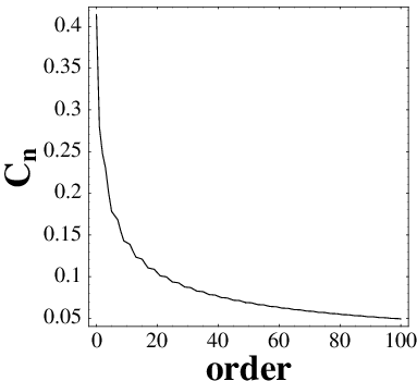
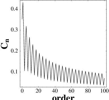
Let us consider two cases, as before: one where is small and one where is large, as near the interaction points of large colliders. For the first case ( small), we may neglect the terms having as a factor in the coefficient and in the second case, we can pull out from the square root and neglect terms in the coefficient having now the function in the denominator. In this way, the coefficients of Eq. (30) will depend only on the order . We plot in Figs. 1, the behavior of these coefficients as a function of the multipole order , for large and small . The dominant factor in seems to be , which is reflected in the slow asymptotic decay depicted at the plots. For all practical cases (multipole orders up to 20), lies between 1/2 and 1/10. Assuming now that the average in the body of the magnet is not so different from in the fringe, one gets for small functions:
| (31) |
as in Eq. (25), and for large:
| (32) |
as in Eq. (26).
IV.3 Dipole magnet
Consider a “straight” dipole magnet; the configuration of poles and coils is symmetric about the and planes, and the coils are excited with alternating signs and equal strength. By symmetry is odd in both and , is even in both and , and is even in and odd in . Using the general field expansion of Eq. (9), we get:
| (33) |
Taking the field expansion up to leading order, we get:
| (34) |
where represents a sextupole field component allowed by the symmetry of the “dipole” magnet (for an ideally designed magnet ) and contain all the allowed terms of higher orders.
A point has to be made about the application of the integrals evaluating the rms momentum kicks for bending magnets: because of the curved central orbit, these integrals are not exact, as previously mentioned. Nevertheless, in most practical cases, the field uniformity in the interior of a “dipole” magnet is very high, and thus, on heuristic grounds, this approach can be expected to provide fairly good estimates even in this case.
The change of transverse momentum imparted by the dipole field is (see Eq. (15))
| (35) |
where as before is the effective length of the “dipole” magnet, and is the main dipole field in the body of the “dipole” magnet. Using Eq. (18) the deflections in one fringe are
| (36) |
and the total r.m.s. fringe kick is
| (37) |
Using Eqs. (68) and (69), we have
| (38) |
and the r.m.s. transverse momentum kick becomes
| (39) |
Thus, the by-now-standard ratio is
| (40) |
Except for numerical factors near one this formula yields the same “ball-park” estimates as given by Eq. (31) and Eq. (32) for the small and large cases.
IV.4 “Quadrupole” magnet
The configuration of poles and coils in a “quadrupole” magnet is symmetric about the four planes and if the coils are excited with alternating signs and equal strength, the magnetic field will satisfy the following symmetry conditions: is even in and odd in ; is odd in and even in ; is odd in both and ; and . As before, we may express the field components as:
| (41) |
The field expansion can be written as
| (42) |
where is the transverse field gradient at the quadrupole axis, and contain all the higher order terms. For a particle traversing the magnet with a horizontal deviation and vertical deviation from the center, the momentum increments produced by the nominal field gradients are
| (43) |
where is the effective length of the quadrupole magnet. The momentum increments of the particle contributed from the longitudinal component of the magnetic field are
| (44) |
and the momentum increment produced by the transverse component of the fringe fields are
| (45) |
Combining the contributions, the total momentum increments due to fringe field are
| (46) |
Again, by averaging the sum of squares of the transverse momenta contribution, we obtain the total rms transverse momentum kick imparted by the fringe field:
| (47) |
Note that the expected rotation symmetry of the quadrupole is exhibited both in this formula and in the body deflection formula. The standard ratio is
| (48) |
Again dropping factors near 1, this leads to the same ball-park estimates of Eq. (31) and Eq. (32) .
IV.5 Magnets of LHC and SNS
The LHC and the SNS accumulator ring are good examples for testing the validity of the derived fringe field figure of merit formulas. Indeed, the purpose of these two proton machines and thereby their magnet design differs in great extent: the LHC, a high-energy hadron collider, is filled with long super-conducting magnets of very small aperture (around 1 cm). In contrast, the SNS ring, a low-energy high intensity accumulator, contains short normal conducting magnets with wide aperture (tens of cm). In addition, the lattice design, optics functions and physical parameters of the two machines are substantially different, e.g. the emittance of the SNS beam is several orders of magnitude bigger, than the one of the LHC. In Table 1, we summarize the parameters of the main magnets in the two accelerators entering in the figure of merit formulas (40) and (48).
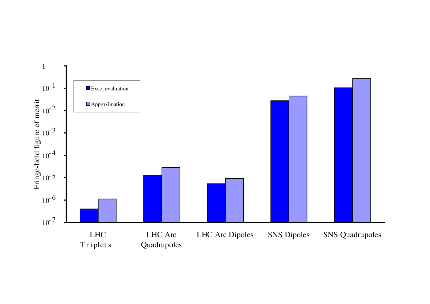
In Fig. 2, we plot in logarithmic scale the fringe-field figure of merit estimates for the LHC and the SNS accumulator ring magnets. The black bars represent evaluation with the exact formulas derived for dipoles and quadrupoles (see Eqs. (40) and (48)) and the grey bars represent the evaluation with the formula for round beams (31). In both cases, the total effect for each magnet is computed by summing up the fringe-field figures of merit from both ends due to all the magnets of the same type. The fringe field importance in the case of the SNS is striking, especially for quadrupole magnets, whereas in the case of the LHC can be completely neglected. Note that similar results can be derived by careful dynamical analysis and computation of tune-shifts due to fringe fields or dynamic aperture analysis for both the LHC Meot and the SNS Papaphilippou. It is important to stress that even the approximate formula for round beams (31) is slightly pessimisitic and within a factor of 2 of the exact figure of merit.
V Conclusion
We have derived formulas for the momentum kicks imparted by the fringe fields of general straight (non-solenoidal) multipole magnets. These formulas are based on an expansion having arbitrary dependence on the longitudinal coordinate. This expansion can be used for direct integration of the equations of motion for particle tracking or other analytical non-linear dynamics estimates. It also permits the fringe part and the body part of individual magnets to be identified and separated. A figure of merit, the ratio of r.m.s. end deflection to r.m.s. body deflection is introduced and evaluated. Its proportionality to the transverse emittance results in an easily-evaluated measure of the importance of fringe fields both in cases in which the variation of optical functions is not too rapid and in the opposite case of rapid variation. These results are in agreement with previous crude estimations which employed simple physics arguments based on Maxwell laws theorem. Finally, the formalism has been applied to the most common cases of multipole magnets, namely normal “dipoles” and “quadrupoles” EPAC2000. Since the straight line approximation has been used throughout, these formulas are only precise for magnetic fields that are well-approximated by step functions (the “hard-edge” approximation). Thus, the formulas contain no parameters associated with the fringe shape (for example, see Venturini; BerzErdelyiMakino). Also, as stated previously, only those fringe fields matching, and therefore required by, the nominal body multipolarity are accounted for.
Numerical evaluation of the end/body figure of merit shows that fringe fields can be neglected in the magnets populating the arcs of large colliders like the LHC. In these rings, the magnets are long enough and the emittances are so small (of the order of m rad) that the effect of fringe fields is a tiny perturbation as compared to the dominant multipole errors in the body of the magnets. The effect may be important, however, in small rings, as the SNS accumulator ring Papaphilippou or the muon collider ring BerzErdelyiMakinoII, where the emittance is large (typically m rad) and the magnets much shorter. Careful consideration should be also taken in the case of the magnets located in the interaction regions of the collider Wan, where the beta variation is quite big.
It is perhaps appropriate to call attention to possible “overly optimistic” use of the scaling law. Often quadrupoles are grouped in doublets or triplets in which the desired focal properties rely on the intentional, highly-tuned, near cancellation of deflections caused by more than one element. In such cases, the fringe deflections are, of course, amplified, when evaluated relative to the gross multiplet deflection. This effect is most obvious at focal points.
Since the early analytical studies of Lee-Whiting LeeWhiting and Forest ForestMilut; Forest, significant progress has been achieved for the construction of accurate maps which represent the motion of particles through the magnet fringe field, using either direct numerical evaluation with exact integration of the magnetic field VenturiniDragt; marylie or parameter fit of an adequate function Hoffstater; ErderlyiLindermann; COSY (e.g. the Enge function Enge). These maps are essential for the study of non-linearities introduced by fringe-fields through Hamiltonian perturbation theory techniques. On the other hand, the scaling law we have emphasized can provide a rough estimate of the impact of these fringe fields in a ring. If the fringe fields are found to be important, a thorough numerical modelling and analysis of their effect has to be undertaken, including computation of the amplitude dependent tune-shift, resonance excitation and dynamic aperture Venturini; BerzErdelyiMakino; Papaphilippou; PEPII; Zimmermann; ZimmermannII; ZimmermannIII; BerzErdelyiMakinoIII, as non-linear dynamics can be very sensitive to the details of different lattices and magnet designs. Furthermore, great care is required to preserve symplecticity and use these maps in particle tracking.
Appendix A 3D MULTIPOLE EXPANSION, CYLINDRICAL COORDINATES
The magnetic field representation in Cartesian coordinates is not optimal for studying symmetries imposed by the cylindrical geometry of a perfect multipole magnet. For this, it is preferable to rely on expansions in cylindrical coordinates Danby; Brown; Bassetti; ForestMilut; Forest; Gardner; VenturiniDragt. Both expansions are equivalent and the use of the former or the latter depends mostly on taste and the specific problem to be treated.
First, consider the magnetic scalar potential written in the following form ForestMilut; Forest
| (49) |
where now the –dependent coefficients are generally complex. The above expansion follows directly from the fact that the Laplacian commutes with Forest. This allows the consideration of solutions where the dependence in is an harmonic -pole. This expansion is compatible with the general solution of the Laplace equation in cylindrical coordinates, involving Bessel functions VenturiniDragt; Jackson; Jain.
Using Eq. (49) and the Laplace equation, one gets that . Moreover, , should vanish for (all terms except the dipole). Finally, we have a recursion relation Forest; Gardner similar to Eq. (4):
| (50) |
where again the superscript in brackets denotes derivatives with respect to . Following these relations, one can show that all coefficients with vanish. Thus, the first non-zero coefficient is (for ). By extending the recursion relation (50) so as to express any coefficient as a function of , we get:
| (51) |
The summation indexes can be rearranged so as to express the magnetic scalar potential in cylindrical coordinates Forest; Kareh:
| (52) |
and the three-dimensional field components are:
| (53) |
The coefficients can be related with the usual multipole coefficients, through Eqs. (6). First, we write the scalar magnetic potential in Cartesian coordinates:
| (54) |
The magnetic field components are computed by the gradient of the potential (54):
| (55) |
Using Eqs. (6), we get:
| (56) |
where the upper limit of both series is the integer part of . Thus, in the absence of longitudinal dependence of the field, the normal and skew multipole coefficients are just scalar multiples of the imaginary and real part of . On the other hand, the situation is more complicated in the case of 3D fields. By inverting the series (56), we have:
| (57) |
where the coefficients and can be computed order by order by the relations
| (58) |
and runs from 1 to the integer part of . Using the last relations, the scalar potential and the magnetic field can be expressed as a function of the usual multipole coefficients. By expanding the complex polynomials in the expression of the magnetic field components, one recovers the expansions of the magnetic fields (9) in Cartesian coordinates.
Appendix B EVALUATION OF R.M.S. END DEFLECTIONS
In order to evaluate the r.m.s. deflection caused by a magnet end, we start from the expressions (21) by splitting the product inside the brackets:
| (59) |
The total r.m.s. transverse momentum kick imparted by the fringe field is , where the operator denotes the average over the angle variables. An equivalent expression stands for the deflection due to the body part of the field. The operator is linear, we can first compute the sum of squares of the momentum kicks and then proceed to their averaging. Thus, we have:
| (60) |
where , and are:
| (61) |
We have the following relations for the real and imaginary part of :
| (62) |
and thus:
| (63) |
where the upper limit of the last sum is taken to be for uniformity in the equations, instead of the last non-zero term for which . Finally, it is straightforward to show that
| (64) |
After expanding the products in Eq. (60) and collecting the terms of equal power in the transverse variables, we have that the transverse kicks can be written in the following form:
| (65) |
where the ’s are
| (66) |
with the coefficients ’s:
| (67) |
In order to proceed to the averaging of the transverse variables, we write them in the standard form
| (68) |
where are the transverse emittance associated with the corresponding phase space dimension, , are the usual beta and alpha functions and stand for , respectively. Using the above relations and averaging over the angle variables one can show that:
| (69) |
Then, the ’s become:
| (70) |
After collecting terms of equal emittances, the r.m.s. transverse momentum kicks can be expressed as:
| (71) |
where the bars on the ’s denote their average values over the body of the magnet. The coefficients , given by
| (72) |
depend on the twiss functions , and on the multipole order . One may note that r.m.s. transverse momentum kick of the fringe is represented by the square root of a polynomial of order in the transverse emittances and as compared to the square root of a polynomial of order representing the body contribution (see also Forest). Thus, their ratio should be proportional to the transverse emittance. This scaling law is indeed exact for the case of the “dipole” and “quadrupole”. For higher order “multipoles”, it is exact for flat and round beams (Sec. IV).
Appendix C Acknowledgements
The authors would like to thank A. Jain for useful suggestions regarding the magnetic field expansions, E. Keil for his criticism in an early version of this work and R. Baartman for many useful comments and discussion. This work was performed under the auspices of the U.S. Department of Energy.
References
- (1) K.G. Steffen, High Energy Beam Optics (Interscience, New York, 1965).
- (2) E. Forest and J. Milutinovic, Nucl. Instrum. Methods 269, 474 (1988)
- (3) E. Forest, Beam Dynamics - A new attitude and framework, (Harwood Acad. Pub., Amsterdam, 1998).
- (4) J. Irwin and C. Wang, Explicit soft fringe maps of a quadrupole, Proceedings of the Particle Accelerator Conference, Dallas, 1995, (IEEE Piscataway NJ, 1996), p. 2376.
- (5) R. Baartman, Intrinsic Third Order Aberrations in Electrostatic and Magnetic Quadrupoles, in Proceedings of the 6th European Particle Accelerator Conference, Stockholm, 1998, edited by S. Myers et al., (Institute of Physics, London and Philadelphia, 1998), p. 1415.
- (6) I.S. Gradshteyn and I.M. Ryzhik, Table of Integrals, Series, and Products, Corrected and enlarged edition, (Academic Press Inc., San Diego, CA, 1980).
- (7) F. Méot, Particle Accelerators, 55, 329 (1996).
- (8) Y. Papaphilippou and D.T. Abell, Beam dynamics analysis and correction of magnet field imperfections in the SNS accumulator ring, in Proceedings of the 7th European Particle Accelerator Conference, Vienna, 2000, edited by J.-L. Laclare et al., (Austrian Academy of Science Press, Vienna, 2000), p. 1453.
- (9) J. Wei and R. Talman, Particle Accelerators 55, 339 (1996).
- (10) J. Wei, Y. Papaphilippou and R. Talman, Scaling law for the impact of magnet fringe fields, in Proceedings of the 7th European Particle Accelerator Conference, Vienna, 2000, edited by J.-L. Laclare et al., (Austrian Academy of Science Press, Vienna, 2000), p. 1092.
- (11) M. Venturini, Scaling of third-order quadrupole aberrations with fringe field extension, in Proceedings of the Particle Accelerator Conference, New York, 1999, edited by A.U. Luccio and W.W.MacKay, (IEEE Piscataway NJ, 1999), p. 1590.
- (12) M. Berz, B. Erdélyi and K. Makino, PRST-AB 3:124001 (2000).
- (13) M. Berz, B. Erdélyi and K. Makino, Fringe-field effects in muon rings, (preprint).
- (14) W. Wan, C. Johnstone, J. Holt, M. Berz, K. Makino, M. Lindemann and B. Erdélyi, Nucl. Instrum. Methods, 427, 74 (1999).
- (15) G.E. Lee-Whiting, Nucl. Instrum. Methods 83, 232 (1970).
- (16) M. Venturini and A.J. Dragt, Nucl. Instrum. Methods 427, 387 (1999).
- (17) A.J. Dragt, D.R. Douglas, F. Neri, E. Forest, L.M. Healy, P. Schütt, J. van Zeijts, MARYLIE 3.0 User’s Manual, University of Maryland, Physics Department Report, 1999 (unpublished).
- (18) G.H. Hoffstätter and M. Berz, Phys.Rev E 54, 5664 (1996).
- (19) B. Erdélyi, M. Berz and M. Lindemann, Differential algebra based magnetic field computations and accurate field maps, (preprint).
- (20) K. Makino and M. Berz, Nucl. Instrum. Methods 427, 338 (1999).
- (21) H.A. Enge, Deflecting magnets, in Focusing of charged particles, volume 2, edited by A. Septier (Academic Press, NY and London 1967).
- (22) E. Forest, D. Robin, A. Zholents, M.Donald, R.Helm, J. Irwin and H. Moshammer, Sources of amplitude dependent tune shift in the PEP-II design and their compensation with octupoles, Proceedings of the 4th European Particle Accelerator Conference, London, 1994, edited by V. Suller and C. Petit-Jean-Genaz, (World Scientific, River Edge NJ 1994), p. 1033.
- (23) F. Zimmermann, Tune shift with amplitude induced by quadrupole fringe fields, CERN-SL-2000-009 AP, 2000 (unpublished).
- (24) F. Zimmermann, C. Johnstone, M. Berz, B. Erdélyi and K. Makino and W. Wan, Fringe fields and dynamic aperture in the FNAL muon storage ring, CERN-SL-2000-011, 2000 (unpublished).
- (25) F. Zimmermann, Fringe fields, dynamic aperture and transverse depolarisation in the CERN muon storage ring, CERN-SL-2000-012 AP, 2000 (unpublished).
- (26) M. Berz, B. Erdélyi and K. Makino, Nucl. Instrum. Methods, 472, 533 (2001).
- (27) G.T. Danby, S.T. Lin and J.W. Jackson, Three-Dimensional properties of magnetic beam transport elements, in Proceedings of the National Particle Accelerator Conference, Washington D.C., 1967, (IEEE Transactions on Nuclear Science 14, No. 3, 1967), p. 442.
- (28) K.L. Brown and R.V. Servranckx, First- and second-order charged particle optics, in Proceedings on Physics of High Energy Particle Optics, BNL/SUNY Summer School, 1983, edited by M. Month, P.F. Dahl and M. Dienes (American Institute of Physics Conference Proceedings No.127, New York, 1985), p. 62.
- (29) M. Bassetti and C. Biscari, Particle Accelerators 52, 221 (1995).
- (30) C.J. Gardner, Three-dimensional field expansions in magnets: A primer, BNL/SNS Technical Note No.53, 1998 (unpublished).
- (31) J.D. Jackson, Classical Electrodynamics, 3rd edition, (John Wiley and Sons, New York, 1999).
- (32) A. Jain, Basic theory of magnets, in Proceedings of CERN Accelerator School on Measurement and Alignment of Accelerator Magnets, edited by S. Turner, (CERN Yellow Report 98-05, Geneva, 1998), p. 1.
- (33) A.B. El-Kareh and J.C. El-Kareh, Electron Beams, Lenses and Optics (Academic Press, New York, 1970).
| Magnet | Number | [m] | [m] | [m] | [m] | [m rad] |
|---|---|---|---|---|---|---|
| LHC Quadrupole Triplets | 16 | 5.5 – 6.37 | 1055 – 4463 | 1157 – 4401 | 1.1 – 203.9 | 5.03 10-10 |
| LHC Arc Quadrupoles | 368 | 3.1 | 32 – 178 | 32 – 176 | 0.5 – 2.4 | 7.82 10-9 |
| LHC Dipoles | 1104 | 14.3 | 28 – 176 | 40 – 143 | 0.5 – 2.6 | 7.82 10-9 |
| SNS Dipoles | 32 | 1.5 | 4 – 8 | 6 | 1.1 – 1.9 | 4.8 10-4 |
| SNS Quadrupoles | 52 | 0.5 – 0.7 | 2 – 28 | 2 – 26 | 0 – 8 | 4.8 10-4 |