Calculation of the Coherent Synchrotron Radiation Impedance from a WigglerPreprint: SLAC-PUB-9628Preprint: January 2003Work supported by the Department of Energy contract DE-AC03-76SF00515
,,Submitted to Physical Review Special Topics—Accelerators and Beams
Abstract
Most studies of Coherent Synchrotron Radiation (CSR) have only considered the radiation from independent dipole magnets. However, in the damping rings of future linear colliders, a large fraction of the radiation power will be emitted in damping wigglers. In this paper, the longitudinal wakefield and impedance due to CSR in a wiggler are derived in the limit of a large wiggler parameter . After an appropriate scaling, the results can be expressed in terms of universal functions, which are independent of . Analytical asymptotic results are obtained for the wakefield in the limit of large and small distances, and for the impedance in the limit of small and high frequencies.
Keywords:
Coherent Synchrotron Radiation; Wakefield; Impedance; Wigglerpacs
29.27.Bd; 41.60.Ap; 41.60.Cr; 41.75.FrI Introduction
Many modern advanced accelerator projects NLC01; TESLA01; LCLS02 call for short bunches with low emittance and high peak current where coherent synchrotron radiation (CSR) effects may play an important role. CSR is emitted at wavelengths longer than or comparable to the bunch length whenever the beam is deflected Warnock90; KYNg90. The stringent beam requirements needed for short wavelength SASE Free-Electron Lasers have led to intensive theoretical and experimental studies CARTor95; Mur97; Derb95; Derb96; DL97; SSY97; RLI99; BraunPRL; BraunPRST; HSK02; HK02; SSY02 over the past a few years where the focus has been on the magnetic bunch compressors required to obtain the high peak currents. In addition to these single-pass cases, it is also possible that CSR might cause a microwave-like beam instability in storage rings. A theory of such an instability in a storage ring has been recently proposed in Ref. SH02 with experimental evidence published in Byrd02. Other experimental observations And00; Abo00; Arp01; Car01; Pod01 may also be associated with a CSR-driven instability as supported by additional theoretical studies JMW98; MW01; VW02.
The previous study of the CSR induced instability assumed that the impedance is generated by the synchrotron radiation of the beam in the storage ring bending magnets SH02. In some cases (e.g. the NLC damping ring Andy02), a ring will include magnetic wigglers which introduce an additional contribution to the radiation impedance. The analysis of the microwave instability in such a ring requires knowledge of the impedance of the synchrotron radiation in the wiggler. Although there have been earlier studies of the coherent radiation from a wiggler or undulator YHC90; Sal98, the results of these papers cannot be used directly for the stability analysis.
In this paper, we derive the CSR wake and impedance for a wiggler. We focus our attention on the limit of a large wiggler parameter because this is the most interesting case for practical applications. It also turns out that, in this limit, the results can be expressed in terms of universal functions of a single variable after an appropriate normalization.
The paper is organized as follows. In Sec. 2, we write down equations for the energy loss of a beam in a wiggler. We then derive the synchrotron radiation wakefield in the limit of a large wiggler parameter in Sec. 3. In Sec. 4, we obtain the synchrotron radiation impedance for a wiggler, and in Sec. 5 we discuss our results.
II Energy Loss and Longitudinal Wake in Wiggler
The longitudinal wake is directly related to the rate of energy loss of an electron in the beam propagating in a wiggler. For a planar wiggler, a general expression for as a function of the position of the electron in the bunch and the coordinate in the wiggler was derived in Ref. Sal98. We reproduce here the results of that work using the authors’ notation:
| (1) |
where is the bunch linear density,
| (2) |
| (3) | |||||
and is the solution of the transcendental equation
| (4) | |||||
In the above equations, we use the following dimensionless variables: and . The parameter is equal to , where and are the projected coordinates on the wiggler axis of the current position of the test particle and the retarded position of the source particle, respectively. The internal coordinate is defined so that the bunch head corresponds to a larger value of than the tail. The wiggler parameter is approximately , with the peak magnetic field of the wiggler in units of Tesla and the period in meters. In addition, is the Lorentz factor, is the electron charge, is the speed of light in vacuum, and is the wiggler wavenumber. Note that the function is a periodic function of with a period equal to . Also note that, desipte assuming , we still assume a small-angle orbit approximation, i.e., .
We introduce the longitudinal wake of the bunch as the rate of the energy change averaged over the coordinate:
| (5) |
where
| (6) |
and we dropped from the list of arguments of the function . The positive values of correspond to the energy loss and the negative values imply the energy gain. The usual longitudinal wake corresponding to the interaction of two particles is then defined as
| (7) |
so that
| (8) |
Note that the wake Eq. (7) is localized in front of the particle and vanishes behind it, for .
In the limit of large , we can neglect unity in the first bracket of Eq. (4), assuming that . Such an approximation is valid, if we are not interested in the very short distances of order of (0.5Å for the NLC damping ring wiggler Andy02). We also introduce a new variable which eliminates the parameter from Eq. (4):
| (9) | |||||
In this limit, the expression for , Eq. (II) can also be simplified:
| (10) |
as long as is not too small, . Again, the parameter is eliminated from this equation. A detailed analysis supporting this approximation can be found in Appendix A.
III Wakefield
Using Eq. (6) and (10) we find
| (11) |
where is implicitly determined by Eq. (9). The integrand in this equation has singularities at points where . It is shown in Appendix B that in the vicinity of a singular point , and the singularity is integrable.
We plot in Fig. 1 the function calculated by numerical integration. A characteristic feature of the function is the presence of cusp points, at which the function reaches local maxima and minima.
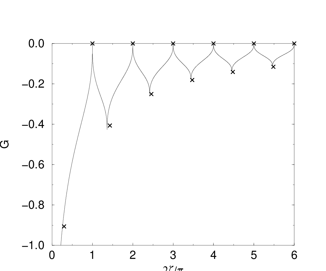
An approximate location of these cusp points and the value of the function at these points can be understood with a simple physical argument presented in Appendix C. It turns out that the minima are located at distances between the particles equal to the integer number of the fundamental radiation wavelength in the wiggler, and the maxima approximately correspond to the distance equal to an odd number of half-wavelength. A simple analytical calculation in Appendix C gives the following results
These are the “” points in Fig. 1, showing very good agreement with the numerical result.
III.1 Short-range limit
In the limit , it follows from Eq. (9) that as well. Eq. (9) can then be solved using a Taylor expansion of the right-hand side:
| (15) |
Expanding the integrand in Eq. (11), keeping only the first non-vanishing term in and substituting from Eq. (15) yields
| (16) | |||||
The above result can also be obtained if one considers a wiggler as a sequence of bending magnets with the bending radius . Indeed, in a bending dipole, the corresponding Mur97; Derb95. Averaging over the wiggler period yields Eq. (16). The reason why such a model gives the correct result in this limit, is that the formation length of the radiation is much shorter than the wiggler period, and one can use a local approximation of the bending magnet for the wake.
III.2 Long-range limit
In the limit , the parameter is also large, and Eq. (9) can be further simplified:
| (17) |
In Eq. (3), we keep only the largest term
| (18) |
For , one now finds,
| (19) |
with
| (20) |
where the function is implicitly determined by Eq. (17). Averaging over one wiggler period, we find
| (21) |
with
| (22) | |||||
It is easy to check that the function is periodic, , and , in agreement with Eq. (III). The average value is equal to . Since is periodic in with a period of , using Eq. (22), we get a Fourier series representation for :
| (23) |
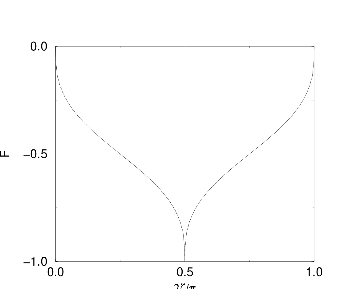
where is the Bessel function of the first kind. Derivations of the Fourier coefficients are presented in Appendix D. In Fig. 2, we plot the function defined in Eq. (23) for one period.
The corresponding long-range wake is then
| (24) |
It is worth noting, that the asymptotic expression in the limit in Ref. Sal98 is incorrect—instead of the -function the authors obtained a sine function, which only corresponds to the fundamental mode of the radiation and neglects contribution from higher-order harmonics.
IV Impedance


The impedance is defined as the Fourier transform of the wake,
| (25) | |||||
where is the wiggler fundamental radiation wavenumber.
We evaluated the integral in Eq. (25) using numerically calculated values of the function in the interval , where and . The contribution to the integral outside of this interval was calculated using asymptotic representations Eqs. (16) and (24).
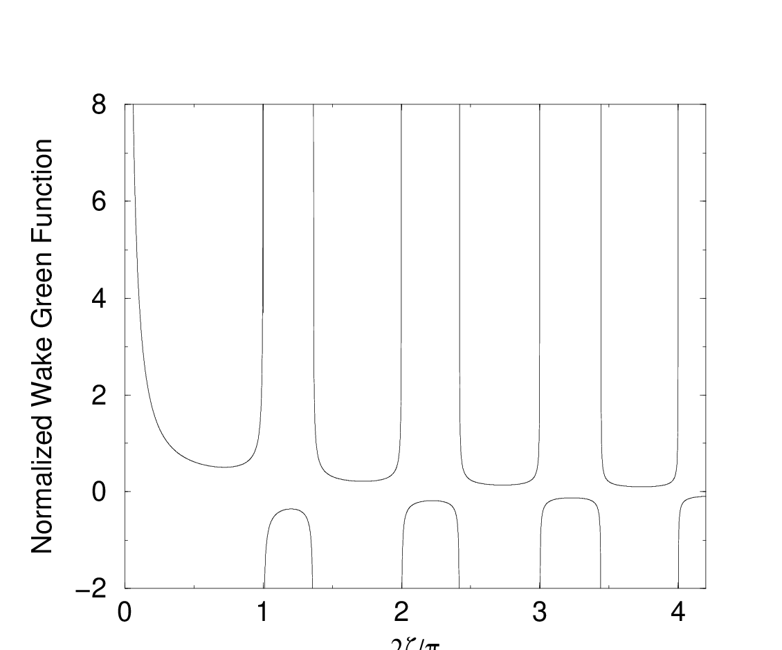
The resulting imaginary and real parts of the impedance are shown in Fig. 4 and Fig. 5 respectively.
The real part of the impedance can be related to the wiggler radiation spectrum Chao93:
| (26) |
The spectrum in the limit is calculated in Appendix E. It shows a perfect agreement with the result presented in Fig. 5.
Simple analytical formulae for the impedance can be obtained in the limit of low and high frequencies.
The low-frequency impedance corresponds to the first term in Eq. (24) for function which does not oscillate with :
| (27) |
Using the definition in Eq. (25), we then obtain the low-frequency asymptotic behavior of the impedance as
| (28) | |||||
where, is the Euler Gamma constant. This asymptotic low-frequency impedance is plotted in Figs. 4 and 5 for comparison with the numerical solution.
V Discussion and conclusion
In this paper, we derived the wakefield and the impedance for wigglers with due to the synchrotron radiation. Analytical asymptotic results are obtained for the wakes in the limit of small and large distances, and for the impedance in the limit of small and high frequencies. The results obtained in this paper are used for the beam instability study due to the synchrotron radiation in wigglers WSRH02.
Acknowledgements.
The authors thank Drs. A.W. Chao, S.A. Heifets, Z. Huang of Stanford Linear Accelerator Center, Drs. S. Krinsky, J.B. Murphy, J.M. Wang of National Synchrotron Light Source, Brookhaven National Laboratory for many discussions. Work was supported by the U.S. Department of Energy under contract DE-AC03-76SF00515.Appendix A Details for deriving Eq. (10)
In the limit of , according to Eq. (3), . In the numerator of the second term on the right hand side of Eq. (II), we would have , as long as . This is allowed, since we are interested in the limit of . Hence, is neglected in the numerator. In the denominator of the second term, then , as long as , hence is dropped. Therefore, the second term of Eq. (II) is on the order of . According to Eq. (4), in the limit of , we have , so the first term of Eq. (II) is on the order of , hence is much smaller than the second term in the limit of . Therefore the first term could be dropped. All these considerations lead us to Eq. (10).
For and , according to Eq. (4), we have . Eq. (3) suggests that . Now, in Eq. (II), in the limit of , we can neglect in comparison with in the numerator and in the denominator of the second term on the right hand side. We then note that the second term is on the order of 1, and is much larger than the first term , hence we can drop to obtain Eq. (10).
Now let us study the limit of . Eq. (3) suggests that . For , then in Eq. (II), and could be dropped in the numerator and denominator of the second term on the right hand side, respectively. The second term is on the order of . Now, according to Eq. (4), in the limit of , we have . Hence, in the limit of , the first term of Eq. (II), which is on the order of , is negligible, compared with the second term. Hence, we obtained Eq. (10).
So, in general, for large , as long as is not too small, i.e., , the simplification leading to Eq. (10) is always acceptable.
Appendix B Singular points in
To find the scaling of the singularity, we assume that at the vicinity of the zeroes of , the leading term scales as
| (30) |
then we have
| (31) |
where the prime indicates the derivative with respect to .
Let us first calculate . From Eq. (3) we have,
| (32) | |||||
To find , we revert to Eq. (9), where, we find
| (33) |
with
| (34) | |||||
Note that is a well defined function at the zeroes of .
Combining Eqs. (30), (32), (33), (34), we have, near the zeroes ,
| (35) |
where,
| (36) | |||||
Here, is defined as the solution of . Therefore, combining Eqs. (35) and (31), we find the scaling index and . This means that has only an integrable singularity at with .
As a numeric illustration of the origin of the singularity, we plot in Fig. 6 functions and for .

Appendix C Simple physics model

Here, we give some explanation about the peaks and the zeroes in Fig. 1 based on a simple physics model.

The CSR wake is actually the field emitted by a trailing particle which acts on the particle in front. Using a model presented in Ref. Derb95, the longitudinal force on the leading particle can be thought of as the component of the trailing particle’s transverse Coulomb field projected onto the leading particle’s direction of motion:
| (37) |
where is the magnitude of the transverse Coulomb electric field at the retarded position from the trailing particle at retarded time. The argument indicates that the amplitude of the transverse electric field is actually varying along the trajectory. In Eq. (37), is the angle between the direction of motion of the trailing particle and that of the particle at front. To illustrate the model, we give a schematic plot in Fig. 7.
To understand the wiggler wakefield, let us look at the four electrons in Fig. 8. The pair with solid arrows is separated by integer number times of the wiggler fundamental radiation wavelength. During their journey, when the light emitted by the trailing electron cathches the electron in front, the instantaneous direction of motion of the front electron is always parallel to the direction of motion of the trailing electron at the retarded time when it emitted the light. Hence we have . So according to Eq. (37), the longitudinal force is always zero. This explains the zeroes in the longitudinal wake potential plotted in Fig. (1). The pair with dashed arrows is separated by odd integer number times of half of the wiggler fundamental radiation wavelength. Averaged over one period, they make the largest angle between the instantaneous direction of motion of the front electron and the direction of motion of the trailing electron at the retarded time. Hence according to Eq. (37), the longitudinal force reaches maximum. This explains the peaks shown in Fig. (1).
Let us calculate the values at these cusps points. According to Eq. (9), when , we have . According to Eq. (11), the numerator of the integrand is zero at , while according to Eq. (3). Hence the integral is zero. So we have for . We find that it is true in the numerical solution in Fig. 1.
At , according to Eqs. (11) and (3), we get
| (38) | |||||
According to Eq. (9), we have
| (39) |
In the above approximation, we average over one period in . This becomes a good approximation, when is large. This manifests itself in Fig. 1. As we find from Fig. 1, with the increasing of , therefore, the increasing of , the above approximate value gets closer and closer to the numerical solution. Combining the results at the zeroes and the peaks, we get Eq. (III).
Appendix D Calculation for the Fourier coefficients
Since we find that the function is periodic in with a period of , we could represent it in a Fourier series. The calculation for the Fourier coefficients are straightforward. We here illustrate one example. For ,
| (40) | |||||
Notice that, we have used the definition of in Eq. (22). We also changed integral variable pair to , using Jacobian obtained from Eq. (17). To complete the integral in Eq. (40), we make use of the well-known identities
| (41) |
with, , for , and
| (42) |
All the other Fourier coefficients, including the average value , are obtained in the same manner. We then obtain the Fourier series representation in Eq. (23).
Appendix E Real part of the impedance and the wiggler radiation spectrum
Our approach to calculate is based on the paper of Alferov et al. Alf73 and that of Krinsky et al. Kri83. The only difference is that we are dealing with large case, hence we could eliminate from the equations as was done for the impedance. Let us illustrate this in the following. The energy radiated per electron per unit solid angle per unit frequency interval per unit length is given by
| (43) |
where is the harmonic number of frequencies in the spectrum. is the number of periods of the wiggler. The polar coordinates and are defined so that, corresponding to the forward direction along the wiggler axis, and to be the plane of electron motion. For a large , is the fundamental radiation frequency, and
| (44) | |||||
where, we define
| (45) |
and
| (46) |
and in turn
| (47) |
and
| (48) |
For finite, but large ,
| (49) |
determines the bandwidth of the radiation. In our theory, we focus on an infinite long wiggler, i.e., we are interested in the limit of . Under such condition, we have . Now we are ready to get the radiation spectrum by integrating over the entire solid angle.
| (50) |
Due to the -function in , the integral over could be done first. Also due to the fact that is small, we approximate . Then the integral in Eq. (50) is reduced into a 1-D integral as the following,
| (51) | |||||
Notice, the integrand has a period of , hence we need only integrate for one period. and are further simplified as
| (52) | |||||
and
| (53) | |||||
Notice is eliminated from this equation, as long as is large. We sum up the first 30 harmonics to obtain the real part of the normalized impedance up to the 4th harmonic. Adding higher harmonics will not change the impedance within this frequency region within numerical accuracy. The result is identical to Fig. 5, supporting the validity of our calculation.
References
- (1) T.O. Raubenheimer, Progress in the Next Linear Collider Design. AIP Conference Proceedings, Vol. 578 P. 53-64, July 9, 2001; NLC ZDR Design Group, SLAC Report-474, Stanford, USA, 1996.
- (2) TESLA: The Superconducting Electron-Positron Linear Collider with an Integrated X-Ray Laser Laboratory, Technical Design Report, DESY, Germmany, March, 2001.
- (3) Linac Coherent Light Source (LCLS) Conceptual Design Report, SLAC-R-593, UC-414, Stanford, USA, April 2002.
- (4) R. Warnock, P. Morton, Part. Accel. 25, 113 (1990).
- (5) K.Y. Ng, Part. Accel. 25, 153 (1990).
- (6) B.E. Carlsten, T.O. Raubenheimer, Phys. Rev. E 51, 1453 (1995).
- (7) J.B. Murphy, S. Krinsky, R.L. Gluckstern, Part. Accel., 57, 9 (1997); J.B. Murphy, S. Krinsky, R.L. Gluckstern, Proc. 1995 IEEE Part. Accel. Conf., P. 2980 (IEEE, Piscataway, NJ 1996); A. Faltens, L.J. Laslett, Part. Accel., 4, 151 (1973).
- (8) Ya.S. Derbenev, et al., DESY Report DESY-TESLA-FEL-95-05, DESY, Germany (1995).
- (9) Ya.S. Derbenev, V.D. Shiltsev, SLAC Report: SLAC-PUB-7181, 1996.
- (10) M. Dohlus, T. Limberg, Nucl. Instrum. Methods Phys. Res., Sect. A 393, 494 (1997).
- (11) E.L. Saldin, E.A. Schneidmiller, M.V. Yurkov, Nucl. Instrum. Methods Phys. Res., Sect. A 398, 373 (1997); G. Stupakov, P. Emma, Proc. 2002 Euro. Part. Accel. Conf., P. 1479 (Paris, France, 2002).
- (12) R. Li, Proc. 1998 Euro. Part. Accel. Conf., P. 1230 (Stockholm, Sweden, 1998); R. Li, Nucl. Instrum. Methods Phys. Res., Sect. A 429, 310 (1999).
- (13) H. Braun, F. Chautard, R. Corsini, T.O. Raubenheimer, P. Tenenbaum, Phsy. Rev. Lett. 84, 658 (2000).
- (14) H. Braun, R. Corsini, L. Groening, F. Zhou, A. Kabel, T.O. Raubenheimer, R. Li, T. Limberg, Phsy. Rev. ST Accel. Beams 3, 124402 (2000).
- (15) S. Heifets, G. Stupakov, S. Krinsky, Phys. Rev. ST Accel. Beams, 5, 064401 (2002).
- (16) Z. Huang, K.-J. Kim, Phys. Rev. ST Accel. Beams, 5, 074401 (2002).
- (17) E.L. Saldin, E.A. Schneidmiller, M.V. Yurkov, Nucl. Instrum. Methods Phys. Res., Sect. A 483, 516 (2002).
- (18) G. Stupakov, S. Heifets, Phys. Rev. ST Accel. Beams, 5, 054402 (2002).
- (19) J.M. Byrd et al., Proc. 2002 Euro. Part. Accel. Conf., P. 659 (Paris, France, 2002); J.M. Byrd et al., Phys. Rev. Lett. 89, 224801 (2002).
- (20) Å. Anderson et al., Opt. Eng. 39, 3099 (2000).
- (21) M. Abo-Bakr et al., Proc. 2000 Euro. Part. Accel. Conf., P. 720 (Vienna, Austrain, 2000); M. Abo-Bakr et al., Phys. Rev. Lett. 88, 254801 (2002).
- (22) U. Arp et al., Phys. Rev. ST Accel. Beams 4, 054401 (2001).
- (23) G.L. Carr et al., Nucl. Instrum. Methods Phys. Res., Sect. A 463, 387 (2001); G.L. Carr et al., Nature 420, 153 (2002).
- (24) B. Podobedov et al., Proc. 2001 IEEE Part. Accel. Conf., P. 1921 (IEEE, Piscataway, NJ, 2002); S. Kramer et al., Proc. 2002 Euro. Part. Accel. Conf., P.1523 (Paris, France, 2002).
- (25) J.-M. Wang, Phys. Rev. E, 58, 984 (1998); J.-M. Wang, C. Pellegrini, Brookhaven National Laboratory Report: BNL-51236 (1979).
- (26) J.B. Murphy, J.M. Wang, Nucl. Instrum. Methods Phys. Res., Sect. A 458, 605 (2001).
- (27) M. Venturini, R. Warnock, Phys. Rev. Lett. 89, 224802 (2002).
- (28) A. Wolski, “NLC Damping Rings: Lattice Parameters, Information and Resources”, (URL: http://awolski.lbl.gov/nlcdrlattice/default.htm).
- (29) Y.-H. Chin, Proceedings, the 4th Advanced ICFA Beam Dynamics Workshop on Collective Effects in Short Bunches, Tsukuba, Japan, Sep. 24-29, 1990; also Lawrence Berkeley National Laboratory Report: LBL-29981, ESG-118, Dec. 1990.
- (30) E.L. Saldin, E.A. Schneidmiller, M.V. Yurkov, Nucl. Instrum. Methods Phys. Res., Sect. A 417, 158 (1998).
- (31) A.W. Chao, Physics of Collective Beam Instabilities in High Energy Accelerators (Wiley, New York, 1993).
- (32) J. Wu, G. Stupakov, T. Raubenheimer, “Impact of the Wiggler Coherent Synchrotron Radiation Impedance on the Beam Instability”. SLAC-Report: SLAC-PUB-9629, (To be submitted to Phys. Rev. ST - Accel. Beams, 2003).
- (33) D.F. Alferov, Yu.A. Bashmakov, E.G. Bessonov, Zh. Tekh. Fiz., 43, 2126 (1973); Eng. transl. in Sov. Phys. Tech. Phys., 18, 1336 (1974).
- (34) S. Krinsky, M.L. Perlman, R.E. Watson, Handbook on Synchrotron Radiation, Vol. 1, P. 65, Edited by E.E. Koch, North-Holland Publishing Company, 1983.