Experimental study of the Ca2 1SS asymptote
Abstract
The filtered laser excitation technique was applied for measuring transition frequencies of the Ca2 B-X system from asymptotic levels of the X ground state reaching . That level has an outer classical turning point of about 20 Å which is only 0.2 cm-1 below the molecular 1SS asymptote. Extensive analysis of the spectroscopic data, involving Monte Carlo simulation, allowed for a purely experimental determination of the long range parameters of the potential energy curve. The possible values of the s-wave scattering length could be limited to be between 250 and 1000.
pacs
31.50.Bc, 33.20.Kf, 33.20.Vq, 33.50.DqI Introduction
In our previous paper O. Allard and A. Pashov and H. Knöckel and E. Tiemann 2002 we reported on an accurate determination of the Ca2 X ground state potential energy curve (PEC) from Laser Induced Fluorescense (LIF) spectroscopy. The study was motivated by the rapid progress in the development of the Ca frequency standard G. Wilpers and T. Binnewies and C. Degenhardt and U.Sterr and J. Helmcke 2002 and the recent photoassociation spectroscopy data on the 1SP1 asymptote Zinner et al. 2000. It was considered as the first step of a comprehensive investigation, which should provide a description of the X state for short and intermediate internuclear distances, thus enabling the precise determination of the long range part of the PEC, for example from photoassociation spectroscopy or from a molecular beam experiment.
The results of the LIF experiments, however, suggested that in the case of Ca2 it might be possible to make a reasonable description of the long range part of PEC already by means of a classical spectroscopy. Here we mean the shallow potential well of the Ca dimer, which lead to thermal population even of the highest rovibrational levels for normal working temperatures (1220 K), so that a single laser scheme could be applied for their excitation. Of great importance is also the possibility to extend the description of the PEC by a long range dispersive expansion already from 9.4 Å O. Allard and A. Pashov and H. Knöckel and E. Tiemann 2002.
For detecting transitions from ground state levels with we applied the Filtered Laser Excitation (FLE) technique, which was used also by Hofmann et al. Hofmann and Harris 1986 for studying the A excited state in Ca2. With this technique we collected spectroscopic information for about 24 highly excited levels of the X state with up to 38. The outer classical turning point of the last observed level with and is at 20 Å and is located on the rotationally reduced potential only 0.2 cm-1 below the molecular asymptote.
Although the FLE resolution was limited by the Doppler broadening, we will demonstrate that combining the data from O. Allard and A. Pashov and H. Knöckel and E. Tiemann 2002 and this experiment, it is possible to reduce the uncertainty of the experimentally determined long range coefficients, and especially C6 to an extent, to compare them with the results of the most recent theoretical predictions Porsev and Derevianko 2002; Moszynski 2001.
In section II we explain the experimental set up and discuss the achieved experimental resolution and uncertainties. Section III summarizes the methods for constructing of the PEC. Analysis of the experimental data are performed in section IV, where we employed a Monte Carlo simulation in order to determine the error limits of the fitted long range parameters of the PEC.
II Experiment
The calcium dimers are obtained in a heat pipe oven already described in Ref. O. Allard and A. Pashov and H. Knöckel and E. Tiemann 2002. The experiments are performed at helium or argon buffer gas under a typical pressure of mbar and an oven temperature of 1220 K. Working with argon as buffer gas enables us to reduce the pressure to a lower value than with helium without reducing the life time of the heat pipe due to solid calcium closing the optical path. In the frequency range accessible by the lasers in our group the most favorable Franck-Condon factors between the levels close to the asymptote of the X state and the levels of the B state () are less than . In order to achieve a sufficient signal-to-noise ratio using Fourier transform spectroscopy a long term stability in the operation of the oven is needed which is not achievable with our present apparatus. In addition, as it was mentioned in Ref.O. Allard and A. Pashov and H. Knöckel and E. Tiemann 2002, the discrete fluorescence is accompanied by a strong background emission due to bound-bound-free and free-bound-free molecular transitions. To overcome this problems we chose the filtered laser excitation (FLE) technique for direct excitation of the levels close to the asymptote of the ground state.
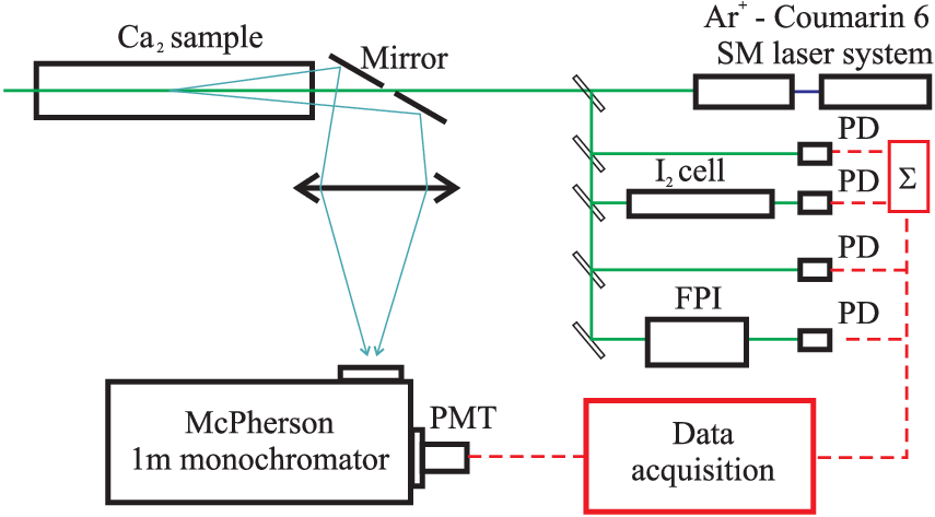
A 1 m monochromator (GCA/McPherson Instruments) used as a narrow band pass filter of a typical window width 2 cm-1 is set on a strong line of the fluorescence progression when exciting a transition to a selected rotational level with of the B state using a single mode dye laser (Coumarine 6). Then the laser operating around 550 nm (60 mW on the Ca2 sample) scans the frequencies of transitions from near asymptote levels of the ground state to the selected level. Laser frequencies resonant with such transitions will result in fluorescence, which matches the transmission band of the filter and can be detected. The signal after the monochromator is recorded as a function of the laser wavelength by a photomultiplier (Hamamatsu, R928). Although many other transitions of the X-B system contribute to the absorption spectrum of Ca2 in the scanned spectral region, only excitations which decay into the selected frequency window will be registered. Thus this selective technique provides greatly simplified absorption spectra in a region where the weak transitions from the asymptotic levels of interest are practically completely overlapped by other much stronger transitions.

The relative positions of the FLE lines are calibrated using the frequency comb of a temperature stabilized Fabry-Perot interferometer with a free spectral range of 149.75(1) MHz. The absolute line position is obtained using the absorption spectrum of iodine vapor at room temperature (fig. 1) calibrated with the IodineSpec calculating software with which the positions of the iodine lines are predicted with an accuracy better than 3MHz in the studied frequency range top; H. Knöckel and E. Tiemann. In order to improve the signal-to-noise ratio each spectrum is recorded several times. Before the averaging procedure, the recorded signal is normalized to the laser intensity to minimize the influence of its variations with frequency and time. The typical width of the observed lines is 0.05 cm-1 corresponding to the Doppler broadening. The intensity of the slowly varying background due to free-bound-free or free-bound-bound transitions of the B-X system is comparable to the intensity of the strongest lines and is mainly responsible for the noise in the spectra. Taking account of the linewidth, the signal-to-noise ratio and the uncertainty in the calibration with the I2 lines, the uncertainty of the absolute frequency for the strongest lines is estimated to be 0.0035 cm-1. Two typical spectra are shown in fig.2 for low and intermediate . The experimental traces as solid lines contain some gaps which were not scanned. The number above the line gives and the inset gives and of the excited state.
Using the FLE technique we observed transitions from 44 ground state levels and among them 24 close to the asymptote with . The last observed levels are (, ) as summarized in the data field in fig. 3. The assignment of the new observed lines is performed using the potential energy curve determined in our previous study of the ground state O. Allard and A. Pashov and H. Knöckel and E. Tiemann 2002 and a numerical potential of the B state determined from the data available in the literature Balfour and Whitlock 1975. Simulations of the transitions by these potentials for selected detection windows are presented in figure 2 as dotted lines. These lines are shifted vertically with respect to the observed traces in order to show clearly the quality of the simulation. The intensity of the synthetic spectrum is determined by the appropriate Franck-Condon factors, by the thermal population of the ground state levels and by the selected detection window. The small differences between the observed and the simulated spectral features could be attributed to the limited accuracy of the B state PEC (0.05 cm-1) and to the fact that the used ground state potential was determined for levels with only . Also, only transitions in the main calcium isotopomer, 40Ca2 were simulated. The unambiguity of the assignment was usually proved further by the observation of relatively long (5-6 vibrational quanta) and self consistent vibrational progressions of P,R doublets.
With the present set-up we can study the influence of the collisions between calcium dimers and the buffer gas by changing its pressure since no additional instrumental broadening on the lines is present. We found that the collisional broadening and the shift of the observed lines are much smaller than what was previously assumed O. Allard and A. Pashov and H. Knöckel and E. Tiemann 2002. This means that the experimental uncertainties of the transitions obtained in that study were overestimated.
For completeness we enriched our data with progressions obtained by LIF using the 501 nm, 488 nm and 457 nm lines of an Argon ion laser (Spectra Physics, BeamLok 2060) recorded by Fourier transform spectroscopy. Most of the transitions which are known to be excited by these lines Vidal 1980 were observed in this study. The present set of transitions representing all the LIF and FLE data covers a range of rotational quantum numbers from to and a range of vibrational quantum numbers from to . We have recorded a total of 3580 transitions resulting in 924 levels of the ground state 11 1 See EPAPS Document No. … for the list of the transition frequencies. This document may be retrieved via the EPAPS homepage (http://www.aip.org/pubservs/epaps.html) or from ftp.aip.org in the directory /epaps/. See the EPAPS homepage for more information.
During this study six atomic calcium lines were also observed around m, which correspond to the 3DP1,2,3 transitions, when irradiating the sample by Ar+ laser lines. These transitions have been already observed in Mg in a similar experiment Scheingraber and Vidal 1977. Here they could be attributed to predissociation of the molecular B state through a coupling with repulsive states correlated to the 3D + 1S asymptotes. It is worth mentioning that the 3DP1,2,3 transitions were observed also at temperatures down to 950 K, which suggests that the first step of the process is predominantly excitation of pairs of free Ca atoms by the laser radiation to the molecular B state. The intensity ratio between the infrared emission and the laser light was highest for the 457 nm Ar+ line and decreases with the increase of the laser wavelength.
After a new examination of the previous Fourier transform spectra using the new potential energy curve which will be presented in the following, three unassigned weak molecular progressions were found to belong to the calcium isotopomer 44Ca40Ca. The exciting transitions were identified as (0, 42)(4, 43) and (0, 72)(5, 73) at 18788.36 cm-1 and (0, 111)(8, 112) at 18787.36 cm-1.

III Construction of PEC
Following the approach adopted in the previous report O. Allard and A. Pashov and H. Knöckel and E. Tiemann 2002, information which concerns only the ground state was extracted from the raw spectroscopic data. From transition frequencies with a common upper state level, differences between ground state levels were calculated. The PEC for the ground state was then constructed, which describes these experimentally observed differences. Similar to Ref.O. Allard and A. Pashov and H. Knöckel and E. Tiemann 2002 the possible combinations of line frequencies within a progression were restricted only to pairs of one P and one R lines, forming a total of 8500 differences.
The methods for construction of PEC were discussed in detail in Ref. O. Allard and A. Pashov and H. Knöckel and E. Tiemann 2002 and will be summarized only briefly here.
The first method represents the potential as a truncated expansion over analytic functions:
| (1) |
where , and are parameters ( is close to the equilibrium distance). For short and long internuclear distances the potential is smoothly extended respectively for with
| (2) |
and for with
| (3) |
Here is the value of the dissociation energy defined with respect to the minimum of the PEC. Since is usually chosen within the region where the contribution of the exchange energy is negligible, no additional dumping (or cut off) functions for the dispersion coefficients are introduced.
Parameters and and are fitted in a nonlinear fitting procedure (for details see Samuelis et al. 2000), while , , and are adjusted by the program in order to ensure smooth connection between the extensions and the analytic form. , and the connecting points and are kept fixed to values, which allow fast convergence of the fitting routine.
The second method defines the PEC for short and intermediate internuclear distances as a set of points connected with cubic spline function. For large internuclear distances the same long range expansion as in (3) is used. The values of the potential in a preselected grid of points, , , and are treated as fitting parameters. They are determined in an iterative fitting routine, which linearizes the problem by using a modified version of the inverted perturbation approach Pashov et al. 2000. The connecting point is chosen in the following way. Initially, the PEC is constructed in a pointwise form up to 13 Å. Then only the long range parameters are fitted assuming that Å. Although both sections of the PEC are determined independently, their shapes turn out to be almost identical between 9.5 Å and 13 Å. As a last step the coefficient of the long range expansion is slightly adjusted (the change does not exceed few percent) in order to fit best the shape of the pointwise potential between 9.4 Å and 10 Å. The crossing point of the pointwise and the long range curves is taken as . The new value of differs from that which was used when fitting the long range parameters. Usually the change is small (typically 0.1 Å) and since the two sections are very close in this region, the effect of such a change on the quality of the fit is negligible. Of course, a second iteration could be performed with the new value of , but usually it is necessary only in the beginning, when the initial values of the fitting parameters are far from the best ones.
Before fitting the PEC to the new data set, the experimental errors of the data obtained by LIF were reanalyzed, since the value of the normalized standard deviation given in the previous study (Ref. O. Allard and A. Pashov and H. Knöckel and E. Tiemann 2002) signals their overestimation. The value of the uncertainty before was chosen to be 0.01 cm-1 for a strong LIF line in order to take into account possible frequency shifts due to collisions. Since the new FLE measurements showed that the probable influence of the temperature and the buffer gas pressure are much smaller than expected we reduced the errors of all LIF frequencies by a factor of 0.6, which will give a more realistic estimate on the error limits of the fitted PEC parameters.
| 3.66 Å | |
|---|---|
| 3.66 Å | |
| cm-1 | |
| cm-1Å12 | |
| 3.66 Å 9.5 Å | |
| -0.5929 | |
| 4.277277 Å | |
| cm-1 | |
| cm-1 | |
| cm-1 | |
| cm-1 | |
| cm-1 | |
| cm-1 | |
| cm-1 | |
| cm-1 | |
| cm-1 | |
| cm-1 | |
| cm-1 | |
| cm-1 | |
| cm-1 | |
| cm-1 | |
| cm-1 | |
| cm-1 | |
| cm-1 | |
| cm-1 | |
| cm-1 | |
| cm-1 | |
| cm-1 | |
| Å | |
| 9.5 Å | |
| 1102.076 cm-1 | |
| cm-1Å6 | |
| cm-1Å8 | |
| cm-1Å10 | |
| Additional parameter | |
| cm-1 | |
| R [Å] | U [cm-1] | R [Å] | U [cm-1] |
| 3.096980 | 9246.6895 | 5.678571 | 636.3741 |
| 3.188725 | 6566.7325 | 5.809524 | 684.9589 |
| 3.280470 | 4525.7282 | 5.940476 | 728.9235 |
| 3.372215 | 3090.9557 | 6.071429 | 768.5976 |
| 3.463960 | 2134.2175 | 6.202381 | 804.2551 |
| 3.555705 | 1475.2425 | 6.333333 | 836.2419 |
| 3.647450 | 1004.5043 | 6.464286 | 864.8746 |
| 3.739195 | 661.4123 | 6.595238 | 890.4666 |
| 3.830940 | 410.6117 | 6.726191 | 913.2923 |
| 3.922685 | 234.0001 | 6.857143 | 933.6417 |
| 4.014430 | 116.0996 | 6.988095 | 951.7718 |
| 4.106174 | 44.5437 | 7.119048 | 967.8632 |
| 4.197920 | 8.6885 | 7.250000 | 982.2159 |
| 4.289664 | 0.1760 | 7.500000 | 1005.2497 |
| 4.381409 | 11.9571 | 7.750000 | 1023.6698 |
| 4.500000 | 48.5948 | 8.000000 | 1038.3262 |
| 4.630952 | 106.9081 | 8.358974 | 1054.3861 |
| 4.761905 | 175.7311 | 8.717949 | 1066.0579 |
| 4.892857 | 248.8199 | 9.076923 | 1074.5969 |
| 5.023809 | 322.3873 | 9.435897 | 1080.8961 |
| 5.154762 | 393.7222 | 9.794872 | 1085.5974 |
| 5.285714 | 461.4555 | 10.303419 | 1090.2990 |
| 5.416667 | 524.6311 | 10.811966 | 1093.5160 |
| 5.547619 | 582.9870 | 11.611111 | 1096.6870 |
| cm-1 | |||
| Å | =3.808 cm-1Å8 | ||
| =1.0023 cm-1Å6 | =5.06 cm-1Å10 | ||
| Additional parameter | |||
| cm-1 | |||
The analytic potential listed in table 1 describes the differences between the observed spectral lines from both experiments with a standard deviation cm-1 and normalized standard deviation =0.69. The quality of the PEC for the near asymptotic levels is estimated by calculation the standard deviation with a reduced set of differences, where for each difference at least one level belongs to . We obtained cm-1 and . The same parameters for the numerical potential (table 2) are cm-1, and cm-1, . In order to calculate the value of the pointwise potential in the range Å, a natural cubic spline through all the grid points should be used. The parameters of both curves are chosen such, that their minima are set to zero. In order to facilitate the comparison between the dissociation energies defined with respect to the lowest rovibrational level (), their values are given in tables 1 and 2 as additional parameters.
IV Uncertainties of the long range parameters
The motivation of this study is not only to describe the rovibrational structure of the 40Ca2 ground state. We rather want to examine to which extent the performed spectroscopic study is able to go beyond the reproduction of the observed differences between ground state levels. Of greatest interest is the reliability of the determined long range parameters (and especially ) since they play an important role in phenomena involving two interacting cold Ca atoms in the ground state.
Our analysis relies on two main assumptions:
- •
the interaction between two Ca atoms can be described within an adiabatic picture, through a single channel model applying the one dimensional Schrödinger equation with an effective potential energy curve;
- •
the shape of the potential for internuclear distances Å can be described with the long range expression (3), neglecting the exchange energy.
Due to the zero net electronic and nuclear spin in the case of 40Ca and the large energy separation between the ground state and the lowest excited states the first assumption seems to be well justified. The second one is supported by the expected small value of the exchange energy Radzig and Smirnov 1985; O. Allard and A. Pashov and H. Knöckel and E. Tiemann 2002 at 9.5 Å and the dominant van der Waals character of the interaction.
Under these assumptions we ask the question: what are the variations of the PEC parameters around the fitted ones which are still in agreement with the experimental data?
In Ref. O. Allard and A. Pashov and H. Knöckel and E. Tiemann 2002 the answer was given by plotting a contour plot of the likehood function by varying the long range parameters. For the nonlinear fitting procedures it is, however, not straightforward how to use the contour plot in order to determine the confidence interval of the parameters since it is not obvious to which confidence limit a given contour corresponds. That is why there is some ambiguity in the probable errors of the fitted parameters determined only by using contour plots. The use of the matrix of variances and covariances, which is obtained by the fitting routines in the linearized form is not useful in our case. The reason is that even if we assume the errors of the experimental frequencies being independent and following a normal distribution, the quantities which enter the fit are actually differences between these frequencies. Consequently their errors are not independent and we are not allowed to interpret the above mentioned matrix as in the case of independent data points.
A possible way to get the probability distribution of the fitted parameters is to perform a Monte Carlo simulation of synthetic data.
IV.1 Monte Carlo simulation
Since our experimental data come with some measurement uncertainties, which we assume to be normally distributed, the set of the fitted parameters of the PEC will differ from the true one . If we perform a series of similar experiments the experimental data sets will be slightly different and consequently we will obtain different sets of fitted parameters . Having a sufficient number of measurement sets we could plot the distribution of and then decide what are the most probable values and what are their uncertainties.
| This study | Other sources | |
|---|---|---|
| , cm-1 | 1095.0(5) Vidal 1980 | |
| 1102.08(9) O. Allard and A. Pashov and H. Knöckel and E. Tiemann 2002 | ||
| , cm-1 | 1069.868(10) | 1069.88(9) O. Allard and A. Pashov and H. Knöckel and E. Tiemann 2002 |
| cm-1Å6 | 1.003(33) | 1.070(6) Porsev and Derevianko 2002 |
| 1.098 Moszynski 2001 | ||
| 1.15 Vidal 1980 | ||
| O. Allard and A. Pashov and H. Knöckel and E. Tiemann 2002 | ||
| cm-1Å8 | 3.27 Moszynski 2001 | |
| O. Allard and A. Pashov and H. Knöckel and E. Tiemann 2002 | ||
| cm-1Å10 | 4.74 Moszynski 2001 | |
| O. Allard and A. Pashov and H. Knöckel and E. Tiemann 2002 |
So let us assume that the fitted potential , described with a set of parameters , is not too far from the true one. Then, knowing the experimental uncertainty associated with each observed transition frequency, we can synthesize a set of experimental data which will have exactly the same structure as the real one (measurement errors, distribution of and quantum numbers). For this goal transition frequencies are formed using the eigenvalues for (since the upper state levels play no role in our analysis their energies could be set to zero) and adding to each calculated frequency a small random quantity normally distributed with mean value zero and a standard deviation equal to the experimental error. Then we transform the synthetic frequencies into synthetic differences and use the same fitting procedure in order to obtain a new set of parameters . Performing a large number of simulations we can plot the distribution of . Since the simulated data are related statistically to in the same way as the real experimental data to the true potential and since these two potentials were assumed to be close to each other the obtained distribution should be not too different from that of .


In order to realize these ideas we used the pointwise representation of the potential since in the present realization of our computer codes it allows more flexibility in connecting the long range expansion with the potential curve at intermediate internuclear distances. The prize to pay for this is that the first derivative of the PEC might have a small “kink” in . This problem, however, does not influence the analysis of the PEC and it could be avoided by slight adjustment of the pointwise curve. What we win is that all the long range parameters are fitted to the experimental data independently of the actual shape of the potential at intermediate internuclear distances. The continuity of the potential is ensured mainly by varying the connecting point and to a smaller extend . Analysis similar to those, performed in Ref. O. Allard and A. Pashov and H. Knöckel and E. Tiemann 2002 showed that the present body of experimental data fixes the inner part of the PEC approximately between 3.5 Å and 9.5 Å. Possible variations in this region are connected mainly with the experimental uncertainties and the influence of the selected representation for the potential is negligible. Therefore we may expect that the choice of the connecting point around 9.5 Å makes our analysis almost independent of the functions used to model the PEC at short internuclear distances.
Having generated a set of synthetic differences we treat them as the experimental data. is taken as initial potential and a small correction to it is fitted which should minimize the difference between and the differences calculated with the corrected potential. The correction is defined as follows:
| (4) |
and
| (5) |
where are defining functions of the pointwise potential (see Pashov 2000), are the values of the correction in an equidistant grid of internuclear distances and , , , are the corrections to the long range parameters. Using the theory of perturbations the shift of the difference due to can be written as:
| (6) |
where
| (7) |
| (8) |
are the corresponding mean values of and calculated with the wave functions of the levels forming the difference.
Note that in principle the exact presentation of is not of importance since we study only the possible small variations around it which are still allowed by the experimental data. The advantage of expressing the correction to the potential in a pointwise form (cubic spline function is used for interpolation) is that the influence of the parameters is localized in , since away from decays exponentially Pashov et al. 2000. This gives a high flexibility in constructing the needed form of the correction. Additionally, the correlations between are introduced mainly by the experimental data and not by the selected basis functions.
With each set of simulated data a new fit is performed which adjusts , , , and . Along with this we examine the contributions due to and the long range corrections to the fitted differences (the sums in Eq. 6). As it could be expected, the changes of the PEC for are very small ( cm-1) for all sets of synthetic data due to the large amount of experimental observations in this region. In addition the corrections to the differences due to , i.e. the first term of the right side of eq. 6, turn out to be smaller than the corresponding experimental uncertainties and in principle one could neglect them. We checked this and, indeed, the distribution of the long range parameters was almost identical for simulations with and without fitting . Since this is true for different numbers of parameters, we may consider it as a proof of the statement made above, that in the present case the determination of the long range parameters is almost independent on the model used to describe the inner part of the PEC.
The positions of the energy levels and the molecular asymptote in Ref. O. Allard and A. Pashov and H. Knöckel and E. Tiemann 2002 were defined with respect to the minimum of the PEC, . Then we estimated that the possible variation of for different representations of the potential is of the order of 0.01 cm-1, which was smaller than the uncertainty of the dissociation energy, 0.09 cm-1. With the extended experimental data set and after the revision of the experimental uncertainties we are now able to give a much better prediction of the dissociation energy with uncertainty also of the order of 0.01 cm-1. Obviously defining the dissociation energy with respect to will introduce an undesired increase of the uncertainty for this long range parameter. Consequently, starting from here we will consider only the value of the dissociation energy defined with respect to the lowest rovibrational level . Indeed, fitting to the simulated data we convinced ourselves that although the shape of the potential (and also ) could vary slightly from fit to fit, the overall effect on the position of is much smaller than the typical variation of . Nevertheless, the contribution of to the uncertainty of is taken into account.
In this way, the main steps of the performed Monte Carlo analysis are:
- 1.
Find the PEC which can reproduce the experimental observations with smallest standard deviation;
- 2.
From the eigenvalues for generate a set of synthetic data by adding normally distributed random deviations according the experimental uncertainties. This set has exactly the same structure as the experimental data;
- 3.
Perform a fit with the synthetic data as it was done with the original one and collect the obtained potential parameters in a distribution list;
- 4.
Repeat steps (2)-(4) until enough simulated long range parameters are collected in order to analyze their distribution.
IV.2 Results
In figure 4 two projections of the long range parameters distribution obtained from 3000 simulations are shown. It is worth mentioning the strong correlation between and , which is the case also for the other pairs of dispersive coefficients. In order to determine the confidence regions for the parameters we construct an ellipse in the four dimensional space of the parameters, whose axes have such orientations and relative lengths that the resulting surface follows the form of the distribution. Then we change gradually the lengths of the axes by a constant factor and count the number of points which are enclosed by the ellipse. For example, the ellipse which contains 68.3 % of the points will determine the 68.3 % (1) confidence region of the parameters. The projections of the 68.3 % and the 90 % confidence regions (strictly speaking the contours surrounding the projections) are plotted in the left part of figure 4 for the pair of parameters and .
This allows us to determine the mean value and uncertainty of the dissociation energy of the 40Ca2 ground state with respect to the lowest rovibrational level as cm-1 and of the coefficient as cm-1Å6 at a confidence limit of 68.3 %. The values and the uncertainties of all the long range parameters are summarized in table 3 and compared with the values from other sources.

The highest observed rovibrational level in Ref. O. Allard and A. Pashov and H. Knöckel and E. Tiemann 2002 had and it was concluded that with the available experimental data set it is not possible to give any reasonable estimation for . Now, by using a Monte Carlo analysis we can be more rigorous. In figure 5 we compare the projections of two distributions on the - plane. The first one is derived using only the data from Ref. O. Allard and A. Pashov and H. Knöckel and E. Tiemann 2002 before the revision of those experimental errors. In order to obtain a meaningful estimation of the dissociation energy of the X state, we restricted in Ref. O. Allard and A. Pashov and H. Knöckel and E. Tiemann 2002 the possible variation of C6 within a 5 % interval around the theoretical value Porsev and Derevianko 2002. This interval is denoted in fig. 5 with horizontal dashed lines and leads to an uncertainty of the dissociation energy similar to that, given in Ref. O. Allard and A. Pashov and H. Knöckel and E. Tiemann 2002. After including the new LIF and FLE data the distribution shrinks to the small black spot in the centre of figure 5 (see also the inset), which is actually the distribution from figure 4. It would be, however, not correct to interpret the drastic reduction of the size of the distribution only as a result of the transitions involving rovibrational levels with . In fact the items, which led to the distribution presented in figure 4 are:
- •
The assumption that the long range expansion (3) is valid starting from 9.4 Å. This allows to link the values of the long range parameters with the frequency differences involving levels with , i.e. the shape of the long range potential is roughly tested from 9.4 Å up to Å (the classical turning point of the last observed level). A Monte Carlo simulation shows (figure 6) the change of the distribution when shifting from 9.4 Å only by 0.6 Å to Å. Note, that in this case the loss of accuracy on is larger by a factor of two compared to the increase of the uncertainty;
- •
Availability of highly excited levels with , since they limit the variation of the dissociation energy;
- •
The enlargement of the experimental data, which allow accurate determination of the PEC for short and intermediate internuclear distances. Because of the large body of data, the long range parameters are almost independent of the exact representation of the rest part of the PEC, which is clearly indicated by the small variations of (eq. 6) during the statistical analysis;
- •
The corrected estimate of the experimental uncertainties of the data in Ref. O. Allard and A. Pashov and H. Knöckel and E. Tiemann 2002.

IV.3 The value of the coefficient
The confidence interval for given in this paper cm-1Å6 does not overlap with the most recent theoretical prediction of cm-1Å6 within the error stated in Ref. Porsev and Derevianko 2002.
From our side, we realize that an important point in our analysis is the assumption for the validity of the long range expansion (3) down to Å. As it was shown in fig. 6, shifting to larger internuclear distances will increase the uncertainty on the fitted parameters. The same will happen if we introduce additional terms into the long range model (for example the exchange energy). Our analysis can readily include these additional parameters, provided there are new experimental observations which require this.
IV.4 The s-wave scattering length
In order to obtain the s-wave scattering length and its confidence interval, it is straightforward to calculate its value for each of the simulated PEC. These calculations will show how reliably the spectroscopically determined potential up to Å can be applied to model cold collisions. The results are presented in fig. 7a. The position of the last bound level () with respect to the molecular assymptote, is shown in fig. 7b. The values of the scattering length within the 68.3 % confidence region vary from to (the Bohr radius Å). Since these values indicate a bound level very close to the asymptote (several MHz, see fig. 7b),initially we were surprised that from our much less accurate data (several 100 MHz) we can make such a good prediction of the position of the last bound level. Obviously the large amount of observed data fixes the accumulated phase of the wave function for this level along the PEC up to Å and the variation of the binding energy with respect to the asymptote is restricted mainly by the uncertainty of . In addition, from figure 7b we see that the smaller the binding energy, the less sensitive it is to the uncertainties of the other long range parameters.


The inner wall of the potential ( Å), however, is not well fixed by the experimental data. Could its change shift the last level by several MHz without influencing the positions of the other levels? The answer is negative. The wave functions for small internuclear distances for the highly excited levels differ only by a constant factor. For example, for a PEC with binding energy MHz for , the shapes of the wave functions for and are almost identical up to 7.5 Å and the ratio between them is:
| (9) |
So, using the perturbation theory it is clear, that a change of the potential for Å, which will shift the position of the level with by 1 MHz will shift the level with by GHz (0.04 cm-1). Since this change will not alter for example the position of the lowest level (), the introduced shift of the difference will exceed the experimental uncertainty roughly by a factor of 6, which is a contradiction.
Due to the revised confidence interval for the , the uncertainty of the scattering length was not reduced compared to Ref. O. Allard and A. Pashov and H. Knöckel and E. Tiemann 2002 (), although the uncertainty of itself is smaller than the assumed one in Ref. O. Allard and A. Pashov and H. Knöckel and E. Tiemann 2002 ( % around the theoretical prediction of cm-1Å6 Porsev and Derevianko 2002). Following the dependence of the binding energy on the last level on (fig. 7b) we see that for smaller values of this level approaches the asymptote, which makes an accurate determination of the scattering length more difficult.
V Conclusions
The 1S+1S molecular asymptote of the Ca dimer was studied by employing the filtered laser excitation technique. The spectroscopic data obtained in our previous study by Fourier transform spectroscopy were enriched by adding 56 transition frequencies from ground state levels with up to 38. This gave us an opportunity to reanalyze the existing description of the long range part of the PEC from Ref. O. Allard and A. Pashov and H. Knöckel and E. Tiemann 2002.
By assuming the long range expansion (3) for the potential energy curve to be valid already from 9.4 Å, the probability distributions of the dissociation energy and the dispersion coefficients were derived from Monte Carlo analysis. Their mean values and uncertainties are given in Table 3. We showed, that due to the large amount of experimental data, the long range analysis is almost independent of the model functions used to describe the inner part of the PEC.
The reliability of the experimental potential for describing collisions between two Ca atoms at low temperatures was checked by calculating the s-wave scattering length and the position of the last bound level with respect to the asymptote for the variety of long range extensions of the potential allowed by the present experimental data. Following the distribution of the long range parameters, the binding energy of the last level was found to vary between several 10 kHz and several MHz. This confirmed our anticipations O. Allard and A. Pashov and H. Knöckel and E. Tiemann 2002 for a large and positive scattering length, . Contrary to the previous study, the present determination is purely experimental and does not rely on the theoretical estimations for C6. Moreover, the difference in the values of C6 from Ref. Porsev and Derevianko 2002 and from this study exceeds the stated uncertainties, although a small model dependence is still existing by altering the connecting point between the inner potential and the long range branch (compare fig. 6).
The Monte Carlo simulations open new perspectives for analyzing the uncertainties of the parameters of the PEC. They could be used also to determine the kind of spectroscopic data and their required accuracy for achieving the desired uncertainty of the fitted parameters. For example, we checked that including a vibrational progression up to with the present experimental accuracy will not reduce the uncertainties of C6 and D0 significantly. This could be reached, however, even with the present distribution of data, provided the accuracy can be improved. Therefore, we believe that only high resolution Doppler free spectroscopic techniques should be used for further improvement on the Ca2 ground state PEC, especially at long internuclear distances.
VI Acknowledgments
This work is supported by DFG through SFB 407. The authors appreciate the assistance of St. Falke during the experiments. A. P. gratefully acknowledges the research stipend from the Alexander von Humboldt Foundation.
References
- O. Allard and A. Pashov and H. Knöckel and E. Tiemann (2002) O. Allard and A. Pashov and H. Knöckel and E. Tiemann, Phys. Rev. A in print, (2002).
- G. Wilpers and T. Binnewies and C. Degenhardt and U.Sterr and J. Helmcke (2002) G. Wilpers and T. Binnewies and C. Degenhardt and U.Sterr and J. Helmcke and F. Riehle, arXiv:physics/0205049 , (2002).
- Zinner et al. (2000) G. Zinner, T. Binnewies, F. Riehle, and E. Tiemann, Phys. Rev. Lett. 85, 2292 (2000).
- Hofmann and Harris (1986) R. T. Hofmann and D. O. Harris, J. Chem. Phys. 85, 3749 (1986).
- Porsev and Derevianko (2002) S. Porsev and A. Derevianko, PRA 65, 020701(R) (2002).
- Moszynski (2001) R. Moszynski, Private communication (2001).
- (7) IodineSpec can be found on the web site www.toptica.com.
- (8) H. Knöckel and E. Tiemann, Private communication.
- Balfour and Whitlock (1975) W. J. Balfour and R. F. Whitlock, Can. J. Phys. 53, 472 (1975).
- Vidal (1980) C. R. Vidal, J. Chem. Phys. 72, 1864 (1980).
- Scheingraber and Vidal (1977) H. Scheingraber and C. Vidal, J. Chem. Phys. 66, 3694 (1977).
- Samuelis et al. (2000) C. Samuelis, E. Tiesinga, T. Laue, M. Elbs, H. Knöckel, and E. Tiemann, Phys. Rev. A 63, 012710 (2000).
- Pashov et al. (2000) A. Pashov, W. Jastrzȩbski, and P. Kowalczyk, Comput. Phys. Commun. 128, 622 (2000).
- Radzig and Smirnov (1985) A. A. Radzig and P. M. Smirnov, Reference Data on Atoms, Molecules and Ions (Springer, Berlin, 1985).
- Pashov (2000) A. Pashov, Ph.D. thesis, Institute of Physics, Polish Academy of Sciences, Warsaw (2000).