Geometric Random Inner Products: A New Family of Tests for Random Number Generators
Abstract
We present a new computational scheme, GRIP (Geometric Random Inner Products), for testing the quality of random number generators. The GRIP formalism utilizes geometric probability techniques to calculate the average scalar products of random vectors generated in geometric objects, such as circles and spheres. We show that these average scalar products define a family of geometric constants which can be used to evaluate the quality of random number generators. We explicitly apply the GRIP tests to several random number generators frequently used in Monte Carlo simulations, and demonstrate a new statistical property for good random number generators.
pacs
02.50.NgI Introduction
Monte Carlo methods are among the most widely used numerical algorithms in computational science and engineering Dongarra and Sullivan 2000. The key element in a Monte Carlo calculation is the generation of random numbers. Although a truly random number sequence produced by either a physical process such as nuclear decay, an electronic device etc., or by a computer algorithm, may not actually exist, a new and computationally easy-to-implement scheme to investigate random number generators is always highly desirable.
There have been many proposed schemes for the quality measure of random number generators Knuth 1998; W. Press, S. Teukolsky, W. Vetterling, and B. Flannery 1992; Marsaglia 1985; Garcia 2000; Giordano 1997; Gentle 1998; A. M. Ferrenberg, D. P. Landau, and Y. J. Wong 1992; I. Vattulainen, T. Ala-Nissila, and K. Kankaala 1994. These computational tests are based either on probability theory and statistical methods (for example: the test, the Smirnov-Kolmogorov test, the correlation test, the spectral test, and the DieHard battery of randomness tests), or on mathematical modeling and simulation for physical systems (for example: random walks and Ising model simulations). These methods also open the door to studying the properties of random number sequences such as randomness and complexity Kolmogorov and Uspenskii 1987. Some important attempts at an operational definition of randomness were previously developed by Kolmogorov and Chaitin (algorithmic informational theory) Kolmogorov 1998; Chaitin 1987; Chaitin 1990; Chaitin 2001 and by Pincus (approximate entropy) Pincus 1991.
In this paper, we study a new method to measure -dimensional randomness which we denote by GRIP (Geometric Random Inner Products). The GRIP family of tests is based on the observation that the average scalar products of random vectors produced in geometric objects (e.g., circles and spheres), define geometric constants which can be used to evaluate the quality of random number generators. After presenting the simplest example of a GRIP test, we exhibit a computational method for implementing GRIP, which is then used to analyze a number of random number generators. We then discuss the GRIP formalism in detail and show how a random number sequence, when converted to random points in a space defined by a geometric object, can produce a series of known geometric constants. Later we introduce additional members and include them within the GRIP family. We then present the computational results for configurations of four, six, and eight random points, along with a consideration of some key issues. Finally, we conclude by discussing how the GRIP test measures the quality of random number generators by explicitly adding a new quantitative property to random number sequences along with the three known qualitative properties summarized in Ref. Kolmogorov and Uspenskii 1987.
II General Description of the GRIP Formalism
The GRIP scheme is derived from the theory of random distance distribution for spherical objects, and can be generalized to other geometric objects with arbitrary densities Tu 2001; Tu and Fischbach 2002. First, three random points (, , and ) are independently produced from the sample space defined by a geometric object. We then evaluate the average inner product of from two associated random vectors, and . For a geometric object such as an -ball of uniform density with a radius , the analytical result is a geometric constant which can be expressed in terms of the dimensionality of the space Tu 2001; Tu and Fischbach 2002:
| (1) |
A simple derivation of Eq. (1) can be found in the Appendix.
The following procedures are the numerical implementation of our testing programs. A random number sequence produced from a random number generator is used to generate a series of three random points , , and such that these random points are uniformly distributed in an -dimensional spherical ball of radius , where
| (2) |
We then compute a series of values for . If is evaluated times, then statistically we expect
| (3) |
as predicted by Eq. (1).
III Random Number Generators
We now apply the GRIP test to the following random number generators frequently used in Monte Carlo simulations.
- 1.
RAN0 - a linear congruential generator Knuth 1998; W. Press, S. Teukolsky, W. Vetterling, and B. Flannery 1992:
(4) - 2.
RAN3 - a lagged Fibonacci generator Knuth 1998; W. Press, S. Teukolsky, W. Vetterling, and B. Flannery 1992:
(5) - 3.
R31 - a generalized feedback shift register (GFSR) generator Knuth 1998; A. M. Ferrenberg, D. P. Landau, and Y. J. Wong 1992; I. Vattulainen, T. Ala-Nissila, and K. Kankaala 1994:
(6) where is the bitwise exclusive OR operator.
- 4.
durxor - a generator selected from IBM ESSL (Engineering and Scientific Subroutine Library) ess.
- 5.
durand - a generator selected from IBM ESSL (Engineering and Scientific Subroutine Library) and the sequence period of durand is shorter than durxor ess.
- 6.
ran_gen - one of the subroutines in IMSL libraries from Visual Numeric ims.
- 7.
Random - a Fortran 90/95 standard intrinsic random number generator Metcalf and Reid 1999.
- 8.
Weyl - a Weyl sequence generator B. L. Holian, O. E. Percus, T. T. Warnock, and P. A. Whitlock 1994; Tretiakov and Wojciechowski 1999:
(7) where is the fractional part of , and is an irrational number such as .
- 9.
NWS - a nested Weyl sequence generator B. L. Holian, O. E. Percus, T. T. Warnock, and P. A. Whitlock 1994; Tretiakov and Wojciechowski 1999:
(8) - 10.
SNWS - a shuffled nested Weyl sequence generator B. L. Holian, O. E. Percus, T. T. Warnock, and P. A. Whitlock 1994; Tretiakov and Wojciechowski 1999:
(9) (10) where is a large positive integer.
The computational results obtained from Eq. (3) when and are presented in Table 1. Results for random number generators based on other algorithms such as the Data Encryption Standard (DES) Knuth 1998; W. Press, S. Teukolsky, W. Vetterling, and B. Flannery 1992 can be found in Ref. Tu and Fischbach along with the computed results obtained from other geometric objects. We note that both the ran_gen and RAN0 generators perform better overall, while the NWS and Weyl generators (which are based on the Weyl sequence method) are ranked lowest compared to the other generators. The reasons why this is the case will be discussed later.
| Rank | RNG | Error | RNG | Error | ||
|---|---|---|---|---|---|---|
| 1 | ran_gen | RAN0 | ||||
| 2 | RAN0 | ran_gen | ||||
| 3 | R31 | Random | ||||
| 4 | durand | durand | ||||
| 5 | durxor | durxor | ||||
| 6 | RAN3 | R31 | ||||
| 7 | Random | RAN3 | ||||
| 8 | SNWS | SNWS | ||||
| 9 | NWS | NWS | ||||
| 10 | Weyl | Weyl | ||||
| Expected | Expected |
IV GRIP Analysis
In the following, we analyze the relationship between GRIP and a random number sequence, and show how a good random number sequence, when converted to random points in a a space defined by a geometric object, can produce a series of known -dimensional geometric constants. A random number sequence generated from a random number generator can be written as,
| (11) |
When the sequence is converted to represent random points in a -dimensional geometric object, the random numbers in Eq. (11) can then be grouped in pairs as
| (12) |
where Cartesian coordinates are used. The first set of random points can thus be identified as
| (13) |
GRIP then uses , , and to evaluate the average scalar product which can be computed by rewriting,
| (14) |
where is a large positive integer. When the geometric object is a circle of radius and uniform density, we expect as predicted by Eq. (1).
The analysis for -dimensional GRIP can be immediately generalized to the -dimensional case. When the sequence in Eq. (11) is used to generate random points in a -dimensional spherical object, we can regroup Eq. (11) as follows:
| (15) |
The average scalar product of can then be expressed as
| (16) |
When the geometric object is an -ball with a radius and a uniform density, we expect from Eq. (1) that the result of Eq. (16) should be a geometric constant, .
V GRIP Members
For practical computational purposes, we may wish to transform a random number sequence from a uniform density distribution to one which is non-uniform. One of the most important non-uniform density distributions is the Gaussian (normal) distribution with mean zero and standard deviation ,
| (17) |
Here , , and is the space dimensionality. One can use either the Box-Muller transformation method to generate a random number sequence with a Gaussian density distribution, or use available subroutines from major computational scientific libraries such as IBM ESSL and IMSL ess; ims. By applying the probability density function of the random distance distribution as discussed in Ref. Tu and Fischbach 2002, one can add a new GRIP member to investigate the quality of a Gaussian random number generator, and this new GRIP test can be expressed as:
| (18) |
A very common situation arises when one has to produce random points uniformly distributed on the surface of an -sphere of radius . Some general computational techniques for doing this are summarized in Refs. Knuth 1998; Tu 2001. We can then use
| (19) |
to examine the quality of such transformed random number generators as discussed in Ref. Tu and Fischbach.
Another application of the GRIP formalism is in stochastic geometry. We can design a test scheme for a configuration utilizing any number of random points Tu and Fischbach, and these tests can be included in the GRIP family. Among the tests are:
- 1.
Four uniform random points configuration for an -ball of radius
(20) (21) (22) - 2.
uniform random points configuration for an -ball of radius
(23) where ( , etc.) is a positive even number.
A derivation of Eq. (20) can be found in the Appendix. We summarize the computational results for Eq. (23) when in in Tables 2, 3, and 4. A discussion of other results, such as Eqs. (18) and (19), can be found in Ref. Tu and Fischbach.
We observe that all of the generators except NWS and Weyl perform significantly better in than in using the GRIP test based on . We also note from Table 2, and the results (from R31 to RAN0), that these results are clearly biased to larger numbers compared to the expected value. One interpretation may be that is a more sensitive and dedicated computational test for investigating random number generators than other GRIP tests. We also note that the results for are overall worse than , and that the results for reveal a more significant bias than in any of the other cases. These results suggest that the GRIP test either in higher dimensions (large ), or using a configuration of four random points, can serve as a more computationally sensitive test to detect non-random patterns hidden in random number sequences. Finally we note that it is not surprising that the NWS and Weyl generators are ranked worst among all cases in our GRIP test. As reported previously in Tretiakov and Wojciechowski 1999, these two show unacceptable non-random behavior and strong correlations.
| Rank | RNG | Error | RNG | Error | ||
|---|---|---|---|---|---|---|
| 1 | RAN3 | R31 | ||||
| 2 | RAN0 | RAN3 | ||||
| 3 | durxor | SNWS | ||||
| 4 | durand | ran_gen | ||||
| 5 | R31 | durxor | ||||
| 6 | Random | Random | ||||
| 7 | ran_gen | durand | ||||
| 8 | SNWS | RAN0 | ||||
| 9 | NWS | NWS | ||||
| 10 | Weyl | Weyl | ||||
| Expected | Expected |
| Rank | RNG | Error | RNG | Error | ||
|---|---|---|---|---|---|---|
| 1 | durand | SNWS | ||||
| 2 | Random | R31 | ||||
| 3 | RAN3 | ran_gen | ||||
| 4 | ran_gen | durxor | ||||
| 5 | RAN0 | durand | ||||
| 6 | durxor | Random | ||||
| 7 | SNWS | RAN0 | ||||
| 8 | R31 | RAN3 | ||||
| 9 | NWS | NWS | ||||
| 10 | Weyl | Weyl | ||||
| Expected | Expected |
| Rank | RNG | Error | RNG | Error | ||
|---|---|---|---|---|---|---|
| 1 | ran_gen | durxor | ||||
| 2 | durxor | ran_gen | ||||
| 3 | RAN3 | durand | ||||
| 4 | RAN0 | Random | ||||
| 5 | durand | RAN3 | ||||
| 6 | Random | RAN0 | ||||
| 7 | SNWS | SNWS | ||||
| 8 | R31 | R31 | ||||
| 9 | NWS | NWS | ||||
| 10 | Weyl | Weyl | ||||
| Expected | Expected |
VI Conclusions
We have presented a new computational paradigm for evaluating the quality of random number generators. We demonstrate how GRIP helps to understand complexity and randomness by adding a new property, besides three known properties (typical, chaotic, and the stability of frequencies) Kolmogorov and Uspenskii 1987, for random number sequences. This quantitative feature shows how a random number sequence, when converted to random points in a space defined by a geometric object, can produce a series of known geometric constants. Ten random number generators were selected to run our GRIP tests, and they are ranked based on the errors between the numerical and analytical results. Finally we note that one implication of our work is that computational scientists should test the random number generators they use in their simulations, and verify that their random number generators pass as many proposed tests as possible.
*
Appendix A Derivation of and
We derive the analytical result of Eq. (1) for a circle () of radius and uniform density. The same derivation can be applied to the case of dimensions where . We label three independent random points as , , and in Fig. 1, and then calculate
| (24) |
where . From the triangle formed by the random points, we then have
| (25) |
Extending this dimensional case to the -dimensional case, and combining Eqs (24) and (25), we then evaluate
| (26) |
where we have utilized the fact that , , and are three independent random vectors. The functions in Eq. (26), which can be found in Refs. Tu 2001; Tu and Fischbach 2002; Kendall and Moran 1963; Santaló 1976; Solomon 1978; Ambartzumian 1990; Klain and Rota 1997; Fischbach 1996, are the probability density functions for the random distance between two random points in an -dimensional spherical ball of radius and uniform density.
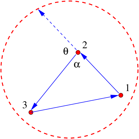
We consider next the analytical result in Eq. (20) for a circle () of radius and uniform density. A similar derivation can lead to Eqs. (21), (22), and (23), as well as to the case of dimensions where . We begin by expressing random points , , , and in Cartesian coordinates, where . The expression in Eq. (20) can then be evaluated by writing
| (27) |
where
A derivation of the general result using the probability density functions in Eq. (26) can be found in Ref. (Tu and Fischbach).
Acknowledgements.
The authors wish to thank T. K. Kuo and Dave Seaman for helpful discussions and the Purdue University Computing Center for computing support. This work was supported in part by the US Department of Energy contract DE-AC02-76ER1428.References
- Dongarra and Sullivan (2000) J. Dongarra and F. Sullivan, Comp. Sci. Eng. 2, 22 (2000).
- Knuth (1998) D. E. Knuth, The Art of Computer Programming Volume 2 (Addison-Wesley, Reading, MA, 1998), 3rd ed.
- W. Press, S. Teukolsky, W. Vetterling, and B. Flannery (1992) W. Press, S. Teukolsky, W. Vetterling, and B. Flannery, Numerical Recipes in C (Cambridge University Press, New York, 1992), 2nd ed.
- Marsaglia (1985) G. Marsaglia, in Computer Science and Statistics: Proc. 16th Symposium on the Interface, edited by L. Billard (1985), pp. 3–10.
- Garcia (2000) A. Garcia, Numerical Methods for Physics (Prentice-Hall, Upper Saddle River, NJ, 2000), 2nd ed.
- Giordano (1997) N. Giordano, Computational Physics (Prentice-Hall, Upper Saddle River, NJ, 1997).
- Gentle (1998) J. Gentle, Random Number Generation and Monte Carlo Methods (Spring-Verlag, New York, 1998), 2nd ed.
- A. M. Ferrenberg, D. P. Landau, and Y. J. Wong (1992) A. M. Ferrenberg, D. P. Landau, and Y. J. Wong, Phys. Rev. Lett. 69, 3382 (1992).
- I. Vattulainen, T. Ala-Nissila, and K. Kankaala (1994) I. Vattulainen, T. Ala-Nissila, and K. Kankaala, Phys. Rev. Lett. 73, 2513 (1994).
- Kolmogorov and Uspenskii (1987) A. N. Kolmogorov and V. A. Uspenskii, Theory Prob. Appl. 32, 389 (1987).
- Kolmogorov (1998) A. N. Kolmogorov, Theoret. Comp. Sci. 207, 387 (1998).
- Chaitin (1987) G. Chaitin, Algorithmic Information Theory (Cambridge University Press, New York, 1987).
- Chaitin (1990) G. Chaitin, Information, Randomness and Incompleteness: Papers on Algorithmic Information Theory (World Scientific, New Jersey, 1990), 2nd ed.
- Chaitin (2001) G. Chaitin, Exploring Randomness (Springer, New York, 2001).
- Pincus (1991) S. M. Pincus, Proc. Natl. Acad. Sci. USA 88, 2297 (1991).
- Tu (2001) S. J. Tu, A New Geometric Probability Technique and Its Applications to Physics, PhD Thesis (Purdue University, West Lafayette, Indiana, 2001).
- Tu and Fischbach (2002) S. J. Tu and E. Fischbach, J. Phys. A: Math. Gen. 35, 6557 (2002).
- (18) eprint http://www.ibm.com.
- (19) eprint http://www.vni.com.
- Metcalf and Reid (1999) M. Metcalf and J. Reid, Fortran 90/95 Explained (Oxford, Midsomer Norton, Avon, 1999), 2nd ed.
- B. L. Holian, O. E. Percus, T. T. Warnock, and P. A. Whitlock (1994) B. L. Holian, O. E. Percus, T. T. Warnock, and P. A. Whitlock, Phys. Rev. E 50, 1607 (1994).
- Tretiakov and Wojciechowski (1999) K. V. Tretiakov and K. W. Wojciechowski, Phys. Rev. E 60, 7626 (1999).
- (23) S. J. Tu and E. Fischbach, in preparation.
- Kendall and Moran (1963) M. G. Kendall and P. A. P. Moran, Geometrical Probability (Hafner, New York, 1963).
- Santaló (1976) L. A. Santaló, Integral Geometry and Geometric Probability (Addison-Wesley, Reading, MA, 1976).
- Solomon (1978) H. Solomon, Geometrical Probability (SIAM, Philadelphia, 1978).
- Ambartzumian (1990) R. V. Ambartzumian, Factorization Calculus and Geometric Probability (Cambridge University Press, New York, 1990).
- Klain and Rota (1997) D. Klain and G. C. Rota, Introduction to Geometrical Probability (Cambridge University Press, New York, 1997).
- Fischbach (1996) E. Fischbach, Ann. Phys. 247, 213 (1996).