In-Vivo NMR of Hyperpolarized 3He in the Human Lung at Very Low Magnetic Fields
Abstract
We present NMR measurements of the diffusion of hyperpolarized 3He in the human lung performed at fields much lower than those of conventional MRI scanners. The measurements were made on standing subjects using homebuilt apparatus operating at 3 mT. O2-limited transverse relaxation ( up to 15-35 s) could be measured in-vivo. Accurate global diffusion measurements have been performed in-vivo and in a plastic bag; the average apparent diffusion coefficient (ADC) in-vivo was , whereas the diffusion coefficient in the bag (3He diluted in N2) was . 1D ADC mapping with high SNR ( 200 - 300) demonstrates the real possibility of performing quality lung imaging at extremely low fields.
Keywords:
Hyperpolarised helium; Lung imaging; Diffusion; ADC.1 Introduction
The first demonstrations of very low field MRI using a hyperpolarized noble gas were done about four years ago, first in glass and plastic cells [1], and subsequently in excised rat lungs [2]. These measurements were performed at 2 mT with a homebuilt instrument, and showed, in convincing fashion, the feasibility of generating MR images with hyperpolarized gas (HG) in magnetic fields that are otherwise far too weak to have produced a useful thermal Boltzmann polarization. There are many possible uses for this technique including medical imaging. In this paper we present a realization of this idea through the first measurements of the apparent diffusion coefficient (ADC) of hyperpolarized in the human lung at very low field (3 mT).
The very first use of HG to image a biological system was reported in 1994; here, the excised heart and lungs of a mouse where imaged using hyperpolarized in a commercial NMR unit operating at 9.4 T field [3]. In-vivo studies on the human lung began in 1996 using conventional clinical systems operating at 0.8 T [4, 5] and 1.5 T [6]. However, unlike conventional MRI, the strong field is not needed here to polarize the gas. Futhermore, if experimental noise is dominated by electrical losses in the body it scales linearly with frequency [7], and because the inductive NMR signal does so as well, the signal to noise ratio (SNR) is independent of field and there exists no benefit to performing HG imaging at high fields in that respect. This was confirmed at 0.1 T by the research group at Orsay using a Sopha-imaging-Magnetech MRI unit [8, 9].
Still, all in-vivo HG studies reported to date have employed high field magnets designed for proton imaging, a fact most likely due to the reason that researchers have found it convenient for the moment to simply adopt existing technology. The question remains, however, at which field strength could HG imaging prove itself most useful for medical diagnostics and will this warrant the development of specialized HG scanners? From this point of view, there are several compelling arguments to investigate very low field ( 0.1 T) HG imaging. We list them here as the underlying motivation for the work presented in this paper.
a) Field Independent SNR - As mentioned, there is no reduction in SNR at lower fields if RF losses in the body dominate the noise. However, below some frequency the body becomes transparent to the RF and the Johnson noise of the detection coils will subsequently dominate. Coil-dominated noise depends on the field as [7], so one expects the SNR to vary as at very low fields. The frequency at which this cross-over occurs has yet to be established experimentally, but it is expected to be larger than the 102 kHz used in our study here. From this point of view, a larger field strength may be preferable, however one should note that a lower than optimal SNR will not necessarily preclude operation in the very low field regime, as there may exist a desirable trade-off with the other possible benefits.
b) Reduced Susceptibility Gradients - Spatial variations in tissue susceptibility produce local field gradients whose magnitude is proportional to the applied field. This can be problematic for lung imaging at high fields, where differences of magnetic susceptibility between blood vessels, lung tissue and airspaces produce very strong gradients.
c) Reduced Power Absorption Rate - RF power absorption rates decrease with frequency. Therefore, operation at lower fields will allow the use of new, rapid pulse sequences without exceeding the safety limit of 4 W/kg of absorbed power. This has been demonstrated at 0.1 T [9] with -pulse repetition times as short as 10 ms.
d) Novel Detection Methods - It may be possible to develop innovative signal detectors that offer improved performance at low field, but would otherwise be impractical for use at high field. Possible examples include networks of local detectors, superconducting coils, and SQUID detectors and amplifiers.
e) Novel Scanner Geometries - Very low field scanners will not require cryogenics (to cool superconducting magnets) nor be encumbered by massive resistive or permanent magnets. This will permit unparalleled flexibility in scanner design. For example, a less bulky system may allow for measurements to be made with the subject either standing or supine, which might be of interest in pulmonary research.
f) Low Cost, Dedicated Scanners for Pulmonary Research - There is strong evidence that the occurrence of certain lung pathologies, such as asthma and chronic obstructive pulmonary disease (COPD), is increasing, and that HG imaging could provide improved diagnosis and assessment of these prevalent afflictions [10]. Should the usefulness of this technique become convincingly established, demands for time on existing conventional scanners could increase dramatically. Very low field, HG scanners should be relatively inexpensive to purchase and operate, and as a result, they might one day find a use in this research area.
Having put forth these proposed benefits, we also point out certain challenges that may exist in performing very low field HG imaging. First, as stated above, SNR will eventually degrade with reduced field. As a result, operating at too low a field would most likely force one to reduce Johnson noise by means of a cryogenic system to cool conventional or superconducting pick-up coils. Another challenge may also arise if one attempts to make ultrafast diffusion measurements or imaging. In this case, the strong applied gradients may have longitudinal and transverse components that approach, or even exceed, the amplitude of the uniform applied magnetic field, thereby precluding straightforward operation [11, 12, 13]. For example, an applied gradient of 15 mT/m would result in additional field components up to mT over the region of the lung; to determine ADC values using such a gradient at very low field (such as 3 mT), one would have to abandon the usual high field approximation and consider a more exact calculation involving diffusion along the line gradient of the total magnetic field [11].
To move well beyond the point of conjecture and to truly examine the potential of very low field lung imaging with hyperpolarized gas, a systematic study of the ideas laid out above must commence. (Additional demonstrations of HG imaging have recently been reported at 15 mT [14]). The goal of our research here was to begin this exploration, first, by developing appropriate apparatus, and second, by performing in-vitro and in-vivo CPMG measurements [15] using hyperpolarized . The results are compared most extensively with those made at 0.1 T [8, 9], as this is the lowest field at which the experimental parameters associated with HG lung imaging have previously been tested.
2 Apparatus
2.1 and Coils
For this first set of measurements, we have employed a previously made magnet. The magnet consists of seven co-axial coils each of 144 turns of 2 mm diameter copper wire wound on an annular aluminum frame. The relative orientation of the coils is shown in cross-section in Figure 1.

The relative homogeneity of the field is only ppm over a typical lung volume (). The magnet was driven by a standard laboratory power supply and could maintain fields up to 6 mT (for 8.7 A, 940 W) without forced cooling. The bore of the magnet is along the vertical (Z-direction), and the entire construction is supported on an aluminum frame (not shown) with the bottom coil being 75 cm above the floor. This provides sufficient room for an average sized person to enter from below and rest standing during measurements.
The subject stands facing the X-direction, with chest centered within the two “C-shaped” coils (shown in Fig. 1) that generate the RF field, , along the Y-direction. These coils were wound on a PMMA (poly(methyl methacrylate)) frame with 11 outer turns (wound A through H) and 9 inner turns (wound B,C,F,G). The outer sections ( = 15.4 cm) make a angle with the inner sections ( = 32.0 cm); the height of the coils is 72 cm and they are separated from one another by a distance = 15.6 cm. The coil was designed (using home-written software) as an inductor to produce an RF field homogeneous to within over a typical lung volume. (This was confirmed by mapping with a small search coil.) To avoid spurious current paths, copper wire with a relatively thick insulating layer (1.4 mm diameter wire covered by a 0.7 mm layer of plastic) was used to keep adjacent windings well separated, thereby minimizing internal capacitance and maintaining a sufficiently high self-resonance of 350 kHz. The coil was tuned to the Larmor frequency with a series capacitor to obtain a convenient low impedance ( , ). It was driven by a homebuilt RF amplifier (with APEX PA46 operational amplifiers) and could produce a -pulse at 100 kHz () in a duration of ms. Gating and dephasing of the RF pulse were controlled via homebuilt circuitry. The reference frequency came from the oscillator output of an EG&G 7265 lock-in amplifier, also used for NMR signal detection.
2.2 Detection Coils
The detection system consists of four rectangular coils: two main coils (each of ten turns and area ) at the front and back of the chest, and two smaller compensation coils (each of forty turns but with the area of the main coils) on either side of the chest. The main coils are separated by 26 cm, the compensation coils by 50 cm. The coils were arranged symmetrically about the center of the coil, and face the X-direction perpendicular to the field. The compensation coils were made smaller due to space limitations inside the magnet, but have the same flux (i.e. area number of turns) as the main coils. They were added to the circuit, as sketched in Figure 2, to increase the signal to noise ratio: the two sets of coils are connected in series, but with opposite polarity, which suppresses external noise signals while augmenting the internal NMR signal.

To measure the NMR signal, the coil system was tuned globally to the Larmor frequency (), and the voltage signal was detected using the lock-in amplifier with differential input.
Typical noise levels at the lock-in output are shown in Figure 3.

The use of the compensation coils reduced the background noise by a factor of 7, which was sufficient to observe the desired NMR signal and make global measurements of the ADC. However, to obtain the necessary resolution for regional measurements, the entire experiment eventually had to be enclosed within a Faraday cage. This brought a further reduction in noise by a factor of 17 as shown in Figure 3. The shielding (0.5 mm copper sheet) was effective in reducing external noise sources to levels below that of the intrinsic noise of the detection system (dominated by the Johnson noise of the coils). Under these conditions, the SNR was slightly better without the use of the compensation coils, as the added noise owing to their large impedance was not offset by their contribution to the signal.
2.3 Gradient Coil for Diffusion Measurements
A gradient coil was made from two pairs of anti-Helmholtz coils (two 7-turn coils separated by 51.6 cm, and two 1-turn coils separated by 20.7 cm) wound on the coil frame. The combination of these coils produces a linear gradient T/m per Ampere. Measurements using a calibrated gradiometer [16] showed the gradient field to be homogeneous to within over the typical lung volume. The gradient coil was driven by a Kepco 50-8M bipolar power supply with current switching times . Eddy-currents generated in the aluminum frame of the magnet have been observed to hamper fast gradient switching by and to have a decay time of . Pre-emphasis was used to compensate for their effect, and the desired gradient is obtained to of the change after and to of the change after
2.4 Gas Production
Production of the hyperpolarized was done in-house using the technique of metastability exchange optical pumping [17, 18]. The gas was polarized at a pressure of about 3 mbar, within a homogeneous magnetic field of 0.9 mT, using a 2W ytterbium fibre laser (Keopsys YFL-1083-20). The pumping was done in a 50 cm long optical cell. The flow of gas through the cell was controlled via the combination of a flow regulator and a peristaltic compressor [19], which is used to extract the polarized gas from the optical cell and accumulate it in a storage cell. With flow rates around 2 of gas at standard pressure per minute, a polarization of could be achieved in the storage cell. Typically, 40 standard of helium (1.8 mmol) were used for each measurement.
3 Method
When the gas was required for an experiment, it was pumped back via the peristaltic compressor into a 1 liter plastic bag (a Tedlar gas sampling bag from Jensen Inert Products) to be carried to the measurement apparatus. High purity nitrogen was used as a neutral buffer gas to inflate the bag with a total amount of gas usually of order 0.5 liter. The relaxation time of the gas in the bag is 20 minutes, so experiments were designed to commence soon after this transfer had been made.
The extraction and transport of the gas was done in earth’s field only, the optical pumping field and the NMR field having both been switched off. Just prior to measurement, and with the bag of gas inside the apparatus, the magnet current was ramped back up. In-vitro measurements were performed in the bag. In-vivo measurements were performed, with governmental approval, using 4 healthy adults who were fully informed about the procedures. While standing within the detection coils, the subject exhaled normally, inhaled the gas directly from the bag, and then further inhaled air to completely fill the lungs. The subject was then required to hold his breath during the acquisition time (typically 5 s or less).
All data presented in this paper were taken at 102 kHz ( mT) using CPMG echo sequences [15]. A RF pulse ( ms) was followed by a train of RF pulses ( ms) to refocus the transverse magnetization at a regular interval . Spatially non-selective tipping was obtained with a good angle accuracy by switching off any applied gradient at least before the beginning of the RF pulses (see App. A). A PC running lab-written software was used to manage the RF and gradient pulse sequencing, as well as to collect data directly from the lock-in amplifier via an A/D converter.
For a CPMG sequence, the transverse magnetization has a decay time
that can be written as
| (1) |
The first term on the right hand side is the inherent relaxation rate of the system, the second term represents additional relaxation resulting from diffusion in a non-uniform magnetic field, due to an applied field gradient and/or the magnet inhomogeneities. For a uniform applied gradient , can be expressed in the case of free gas diffusion as
| (2) |
where is the coefficient of diffusion and the factor corrects for the time variation of the applied gradient, which is switched off during the RF pulses. For a rectangular gradient pulse, this correction factor is given as
| (3) |
where is the duration of the gradient [20].
CPMG measurements were made for different values of (3.6 to 90 ms) and applied gradient (0 to 660 ). For those measurements involving finite , global or regional values of were extracted using Equation 2. This formula remains valid here, since over the length cm of the lung these relatively small applied gradients result in additional longitudinal (transverse) field components that are at least a factor 30 (60) smaller than the uniform 3 mT field [11].
For in-vitro measurements in the bag, this should almost exactly correspond to , the coefficient for free diffusion of in (see App. B). For in-vivo measurements, the extracted value of was considered an apparent diffusion coefficient (ADC) for the restricted diffusion of in the gas mixture inside the lung.
4 Results
Preliminary measurements of the homogeneity were made via NMR on a sealed cell () of low pressure gas. The use of a small set of receive coils gave excellent SNR ( 100) despite the low pressure of the gas (1 to 6 mbar). The gas in the cell was optically polarized in-situ, which allowed the field to be mapped with relative ease. At each position an FID was recorded following a RF pulse; the frequency of the signal gave the local field strength, whereas , the decay time of the FID at of its initial value, gave a measure of local gradients. Measurements were made at fields of 6 mT and 3 mT. In both cases, frequency measurements conformed to the theoretically calculated field map of the magnet. Furthermore, values of were found to be twice as long at the lower applied field, which confirmed that local fields and their gradients were still dominated by the magnet at this level. To minimize residual gradients, we chose to operate at 3 mT or less.
To display the operation of the apparatus as well as some of the characteristics of gas NMR, a collection of CPMG spin echo data is shown in Figure 4.

These measurements were made with the Faraday cage and exhibit excellent SNR’s of 200 to 300. The repetition rate was ms. The time axes of the graphs are broken to accentuate the evolution of the echoes. Data shown in the top panel were taken in-vivo with zero applied gradient, and exhibit an echo amplitude that decays little over the timescale shown ( s). The decoherence time ms (Full Width Half Maximum), and the corresponding spread in the frequency domain, 90 Hz FWHM, are consistent with the inhomogeneity of the field over this volume. This suggests that tissue susceptibility gradients contribute little to the relaxation observed here. Data shown in the middle panel were taken in-vivo with . As a result of the strong applied gradient, the echoes are much more narrow (shorter ) and show a marked decay in amplitude (shorter , now 0.34 s). Data shown in the bottom panel were taken in-vitro with ; to obtain a decay rate similar to that which was observed in-vivo, the value of the applied gradient has to be lowered to compensate for a faster rate of diffusion (see Eq. 2). This result highlights the difference between the restricted diffusion of inside the lung and the free diffusion it experiences in the bag.
Apart from the slowest decays recorded in-vivo (see Sec 4.1), no significant deviation from monoexponential behavior was observed in the diffusion weighted echo decays . To extract values of from our data, monoexponential fits were made to the square of the echo amplitudes, or the square of their Fourier components. The use of power data, rather than the magnitudes, yields a more reliable result as the latter contains a non-zero baseline that leads to an overestimation (underestimation) of decay times if it is left in (subtracted out) [21]. For extremely long decay times, such as those shown in Figure 5, we found that the results from various fitting procedures did not vary significantly (this is further discussed in Sec. 4.3).
4.1 Fast Repetition CPMG with no applied gradient
Measurements made in zero applied gradient using a very short ms are shown in Figure 5.
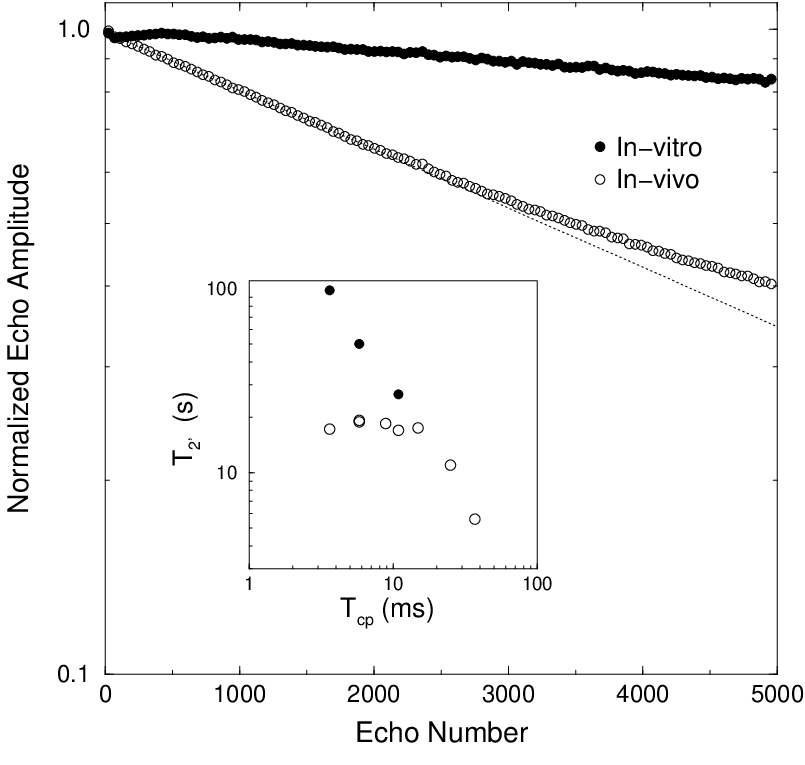
For such a fast repetition rate the lock-in amplifier had to be operated with lower gain which caused a slight decrease in the SNR. The excellent homogeneity of the field allowed for the refocusing of thousands of echoes with very little loss per RF pulse (see App. A). The extremely low power radiated at this frequency allowed these measurements to be safely performed in-vivo as well.
It is clear from Figure 5, that there is marked difference in decay rate between the in-vitro ( s) and in-vivo ( s) results. For in the bag, the transverse relaxation at ms would have been limited by the following: diffusion of the gas in the residual magnet inhomogeneities, -pulse losses, or a combination of both; the longitudinal relaxation, minutes, was too long to have made a contribution. As shown in the inset of Figure 5, the in the bag dropped rapidly with increased indicating that diffusion was the dominant relaxation mechanism above ms. By contrast, the in-vivo hovered around a much lower value (17 - 19 s for this subject, 16 - 22 s for the other three subjects) before falling off at around 15 ms. The values in this plateau region are comparable to the oxygen-limited values ( s) measured for in the lung by MRI at high field [22, 23]. Complementary global measurements of (decays monitored using small angle tipping pulses, as described in Ref. [8]) and (with no applied gradient) have been performed in-vitro at 2 mT in a different NMR apparatus. Decay times of several minutes have been obtained for small amounts of mixed with pure , while 13 s were measured for in air at room pressure and temperature. This strongly suggests that the constant we observed at short was indeed due to the nominal concentration in the lung. To corroborate this finding, similar measurements were made where the subject did not inhale air following a 1-liter bolus of HP gas. In this case, values greater than 30 s and as high as 36 s were observed (for ms), consistent with a longer due to a lower oxygen concentration.
Another strong signature of -induced relaxation can be seen in the main graph of Figure 5. The decay rate in-vivo was not constant, as was seen in-vitro, but instead slowed down over time as the concentration in the lung decreased. This is highlighted by the dashed line which indicates the initial decay rate of 17 s. A full fit to the data (not shown) reveals that the echo decay rate, and hence the partial pressure, decreases linearly with time. This has also been observed by the direct measurement of the in the lung [24].
4.2 Global Diffusion Measurements
A compilation of all our diffusion measurements (taken with and without the Faraday cage, and using two of the subjects only) is shown in Figure 6. These measurements were made with a minimum of 8.8 ms. The general behavior seen here is compared with the recently published results of reference [9] taken at 0.1 T with a different set of two subjects.

The data is plotted as versus , which appears in Eq. (2) as the natural length scale for relaxation due to diffusion. actually differs from the usual pixel size , which sets the resolution of any MR image and provides a useful forum to discuss the results, but the two lengths have similar values in our experiments since .
It is clear from Figure 6 that results at 3 mT (closed symbols) and 0.1 T (open symbols) exhibit the same trend: for a given value of , there is a longer in-vivo owing to the restricted diffusion of the in the small airspaces of the lung. This is fortunate from the point of view of lung imaging, as more time can be had to obtain the desired image resolution. To extract diffusion coefficients, noting that is negligible for these data, linear fits (through the origin) were made to the data of Figure 6 plotted as versus . This procedure gives more weight to measurements with longer which have a higher SNR, and is thus preferred to a linear fit of versus . For in-vitro results, we obtained a value of , in perfect agreement with the expected free diffusion coefficient (see App. B). This is likely to be fortuitous since the gradient calibration is not accurate to better than 1% and the ambient pressure and temperature were not precisely measured during the experiments. The solid line in Figure 6 was drawn using this value to show the theoretical response for the free diffusion of in .
Using all our in-vivo measurements we obtained a value for the global ADC in the lung of , whereas results from reference [9] give (see Tab. 1).
| ADC () | error() | |
|---|---|---|
| all 3mT data | 14.2 | 0.6 |
| 0.1T data | 22 | 1.5 |
| all 3mT data | 11.9 | 3.4 |
| initial 3mT data | 11.3 | 4.2 |
| 3mT data in cage | 12.4 | 2.5 |
| 0.1T data | 16 | 5 |
On average our measurements give a global ADC that is on the order of (the dashed line in Figure 6). In contrast with in-vitro measurements, a possible deviation from quadratic dependence and a large scatter are observed in Figure 6 for in-vivo measurements. The small quoted statistical error on the ADC values in the lung are thus misleading, and it is much more relevant to extract one ADC value from each measurement and to relate the scatter to differences between measurements. The corresponding results are given in the lower part of Table 1. The possible deviation from quadratic dependence in Figure 6 could not arise from the anisotropy of the lung structure at microscopic length scales, as probed using strong bipolar gradients for diffusion weighting [25]. In this experiment, it would rather indicate the complex variation of the gas confinement over the explored length scales (2 - 10 mm). Over the range of diffusion times examined here, the scatter in the data is likely dominated by differences that exist in the physiology of the subjects, and in the degree of lung inflation. In light of these last two points, it is interesting to note that the smallest scatter was obtained for a set of measurements that happened to be taken in a single subject only and where with similar breathing maneuvers were used (data in the Faraday cage, solid circles in Fig. 6).
It is also worthwhile noting that average ADC values reported here and in Ref. [9] tend to be lower than those of other healthy subjects that have recently been measured at 1.5 T using bipolar gradient pulses (17 to from Ref. [26] or 16 to from Ref. [27]). Certainly, physiology and imaging parameters could account for the observed discrepancies, however one should also consider the difference in probed length scales as argued in Ref. [9].
4.3 Regional Diffusion Measurements
Each recorded echo contains information on the distribution of the polarized gas along the applied gradient axis (here, the vertical Z axis oriented from feet to head for a standing subject). FFTs of the spin echoes thus provide series of 1D images with a nominal resolution given by the pixel size defined in the previous section. Provided that the SNR is large enough, a pixel by pixel analysis of the decays can be performed to obtain Z-profiles of the initial gas distribution and of the local decay time. Examples of results of such analyses are shown in Figure 7 for two in-vivo measurements performed with opposite gradient directions.

For each measurement, the fitted initial amplitudes (solid lines) and decay times are obtained from non-linear least squares (NLLS) exponential fits of the power spectra (i.e. fitting, for each pixel, the squares of the amplitudes of the echoes by a single exponential decaying to the noise level). The fitted amplitude profiles are used to compute the actual gas distribution profiles (symbols) by simply correcting for the acquisition system bandwidth (in Fig. 7, the 395 mm field of view (FOV) corresponds to a frequency range of 10 kHz, while the FWHM bandwidth of the detection coil is 5.6 kHz). The SNR in the central region of the lung with highest signal intensity is 180 (signal amplitude in Fig. 7 divided by standard deviation between echoes in similar recordings without polarized gas). The noise level increases near the edges of the FOV due to the growing influence of the amplifier noise in the bandwidth-corrected data.
A difference in profiles obtained for opposite directions of the applied gradient was systematically observed in all experiments, both in-vivo and in-vitro. It is attributed to the rather strong magnet inhomogeneities at the position of the measurements, which result in a non-uniform value of the total gradient. It is much weaker on the field axis, it scales with (as was checked at 1.5 mT) and it is relatively larger at reduced applied . Figure 7 clearly shows that an apparent excess (lack) of signal amplitude is correlated to a longer (shorter) than the average: both effects result from a locally decreased (increased) value of the total field gradient. To first order, the averages of the values obtained from experiments performed with (the filled symbols in Fig. 7) should thus reproduce the true gas distribution profile and the true profile which would be directly measured in a homogeneous field.
A clear non-uniform distribution of the average signal is observed in the high intensity region, however it may result from the imperfectly compensated effects of the measurements. The average profile is quite uniform over most of lung ( over the high signal intensity region), and the observed variations cannot be safely ascribed to actual ADC differences in spite of the high SNR. Regional dependence of the measured ADC in the normal human lung has been observed at 1.5 T [28], with 20% lower ADC values in the posterior part of the lungs of a supine lying subject (this is attributed to the known gravity-induced differences, e.g. of alveolar inflation, in the normal lung). As is discussed in reference [9], the length scale involved in such measurements (typically 0.3 mm) is much smaller than the length scale in a CPMG measurement, and this may impact on the ADC values.
For all measurements performed in the Faraday cage, the high SNR allows to perform a local ADC analysis and to apply the corrections required to obtain local or global values of the ADC. However the reduced SNR of all initial measurements (without the Faraday cage) prevented us from making such corrections, and the global values in Figure 6 have been computed by NLLS exponential fits of the total areas of the power spectra of the echoes. We have checked on all high SNR data (both for and ) that this procedure actually introduces little bias (10%) on the global compared to the true average, much less in fact that the rather large scatter of the in-vivo results.
5 Prospects
In this paper we have presented NMR measurements of in the human lung made with a simple, homebuilt system operating at 3 mT. With this device we were able to demonstrate for the first time some of the proposed benefits of performing HG imaging at very low field, most notably, human scale MR with good SNR using a very simple scanner design. Using a simple wire-wound coil, we were able to generate a field of sufficient homogeneity to observe very long CPMG decay rates without being obscured by -pulse losses or affected by tissue susceptibility effects. Thanks to the full use of the available magnetization in a CPMG experiment, this provides an accurate way to measure the concentration and its time evolution with small quantities of polarized gas. The assessment of the potential interest of these measurements, and their extension to regional measurements must now be performed.
Good SNR was obtained in the 1D profiles even using modest quantities of gas and unsophisticated NMR coils. With additional gradient coils, 2D and 3D imaging is expected to provide results similar to those already obtained in a commercial 0.1 T apparatus [9], with the added flexibility allowed by the ultrafast RF repetition and the very long intrinsic . This potential to perform quality lung imaging and accurate ADC mapping at very low field in a standing subject will be fully used when a dedicated field of adequate homogeneity over the lung volume - a system rather easy to design and build - will be operational.
Appendix A Field inhomogeneities and tipping angle accuracy
In the rotating frame synchronous with the near-resonant component of the RF field, the magnetization tipping at a given point results from the precession during a time around the effective field where is the local Larmor frequency and the frequency of the field. Noting the angle of with the Z direction (that of the average field, see Sec. 2.1), the actual tip angle at position is given by
| (4) |
180∘ pulses cannot be exactly obtained except at resonance (), and the largest tip angle which can be obtained is for the optimal pulse duration We now consider situations where imperfect 180∘ pulses result from small deviations from the resonance conditions and small spatial variations of Setting the pulse duration to its optimal value for the average field (assuming resonance conditions), the tip angle computed from Eq. (4) depends on position through the local values of and as shown in Figure 8.

In our experiment, the RF field is uniform to 3%, and Hz. The field is ramped up just before data acquisition, and the resonance condition at the center of the apparatus is obtained with a reproducibility and a stability of 50 Hz. In the absence of applied gradients, the field inhomogeneity over a typical lung volume is estimated from FFTs of spin echoes such as in Figure 4 (top panel). The 90 Hz FWHM spread (200 Hz spread for 90% of the spectrum area) corresponds to 45 Hz (100 Hz). Finally, when switched gradients are used, their residual value during the RF pulses is lower than 0.5% of the applied value (at most 5 kHz over a 395 mm FOV), i.e. 15 Hz over a lung volume. From the plots in Figure 8, actual angles of 170∘ (160∘) are expected for detunings of 50 Hz (100 Hz). Since angle errors are expected to induce a loss for each pulse in a CPMG sequence [29], the corresponding values for this loss are (). This is consistent with the negligible contribution from pulse losses inferred in all our experiments, even when thousands of echoes are recorded as in Figure 5.
Appendix B Value of in several gas mixtures
The free diffusion coefficient in Eq. (2) depends on the gas temperature , pressure and composition. For helium, there is an additional effect of the isotopic nature. Data have been published for diffusion in helium based on calculations of transport coefficients for accurate potentials [30] and on NMR measurements in [31, 32]. Data for binary diffusion of the - [33, 34] and - [34] systems have been obtained by mass-diffusion measurements. Using a classical theory for transport in dilute gases [35], we provide numerical formulas to compute for a gas with partial pressure in a gas containing other components (, , ) with partial pressure , and , in the simple case of uniform temperature and partial pressures.
We first evaluate the self- and binary-diffusion coefficients of , , , and . With notations of Reference [35],
| (5) |
where is the Boltzmann constant, the atomic mass, the collision cross section in a rigid-sphere model and a -dependent factor depending on the actual interatomic potential. The pressure-independent reduced diffusion coefficient has an apparent temperature dependence (actually assumed in Ref. [32]), but this is not exact for a real gas. For helium ( and isotope mixtures), the computed values in the 200-600 K range [30] can be accurately reproduced (within 0.2%) by a power law For a binary mixture in which (with negligible partial pressure) diffuses in another component is given by Eq. (5) in which the mass is replaced by the reduced mass by (the foreign gas pressure) and depends on the involved interaction potential. The reduced diffusion coefficient again only depends on temperature. For , the values measured in the 300-800 K range [33] can be nicely fit by For both and the ratios of the measurements of reference [34] provide the same exponent 1.68 but this determination is less accurate due to the small temperature interval (300 and 323 K). We thus choose to use the same exponent 1.65 for and All these experimental data have been obtained for , and the faster diffusion of can be evaluated using the ratio of the relevant reduced masses. This procedure provides the correct values within 0.1% compared to the diffusion of helium [30] or helium-hydrogen [36] isotope mixtures. This results from the negligible effect of quantum statistics on the binary collisions at room temperature, and is even more accurate for collisions with a heavier molecule. These isotope effects and the numerical formulas for and are collected in Table 2.
The free diffusion coefficient in a gas mixture is finally given from these reduced diffusion coefficients by :
| (6) |
Eq. (6) can be applied for instance to the gas mixtures used for the in-vitro measurements of Figure 6, for which typically 30 cm3 of were mixed to 1 liter of : for 1 atm at 20 one obtains mm2/s, slightly larger than mm2/s. Eq. (6) can also be applied to evaluate the free diffusion coefficient for typical in-vivo experiments, in which the inhaled dose (30 cm3 of mixed with 0.5 liter of ) mixes with the subject’s lung contents (5 liters of -depleted air, since the typical partial pressure of is 0.13 atm in-vivo instead of 0.21 atm in room air). For 1 atm of this mixture at 37 one obtains mm2/s. This higher value is mostly due to the higher temperature, and to a lesser extent to the faster diffusion of helium in
References
- [1] C.H. Tseng, G.P. Wong, V.R. Pomeroy, R.W. Mair, D.P. Hinton, D. Hoffman, R.E. Stoner, F.W. Hersman, D.G. Cory, and R.L. Walsworth, Low-Field MRI of Laser Polarized Noble Gas, Phys. Rev. Lett. 81, 3785-3788 (1998).
- [2] G.P. Wong, C.H. Tseng, V.R. Pomeroy, R.W. Mair, D.P. Hinton, D. Hoffman, R.E. Stoner, F.W. Hersman, D.G. Cory, and R.L. Walsworth, A System for Low Field Imaging of Laser-Polarized Noble Gas, J. Magn. Reson. 141, 217-227 (1999).
- [3] M.S. Albert, G.D. Cates, B. Driehuys, W. Happer, B. Saam, C.S. Springer and A. Wishnia, Biological Magnetic Resonance Imaging Using Laser-polarized , Nature 370, 199-201 (1994).
- [4] M. Ebert, T. Grossmann, W. Heil, E.W. Otten, R. Surkau, M. Leduc, P. Bachert, M.V. Knopp, L.R. Schad, and M. Thelen, Nuclear Magnetic Resonance Imaging with Hypolarized , Lancet 347, 1297-1299 (1996).
- [5] P. Bachert, L.R. Schad, M. Bock, M.V. Knopp, M. Ebert, T. Grossmann, W. Heil, D. Hoffman, R. Surkau, and E.W. Otten, Nuclear Magnetic Resonance Imaging of Airways in Humans with Use of Hypolarized , Magn. Reson. Med. 36, 192-196 (1996).
- [6] J.R. MacFall, H.C. Charles, R.D. Black, H. Middleton, J.C. Swartz, B. Saam, B. Driehuys, C. Erickson, W. Happer, G.D. Cates, G.A. Johnson, and C.E. Ravin, Human Lung Air Spaces: Potential for MR Imaging with Hyperpolarized He-3 Radiology 200, 553-558 (1996).
- [7] D.I. Hoult and P.C. Lauterbur, The Sensitivity of the Zeumatographic Experiment Involving Human Samples, J. Magn. Reson. 34, 425-433 (1979).
- [8] L. Darrasse, G. Guillot, P.-J. Nacher, and G. Tastevin, Low-field Nuclear Magnetic Resonance in Human Lungs, C.R. Acad. Sci. Paris 324, 691-699 (1997).
- [9] E. Durand, G. Guillot, L. Darrasse, G. Tastevin, P.-J. Nacher, A. Vignaud, D. Vattolo, and J. Bittoun, CPMG Measurements and Ultrafast Imaging in Human Lungs with Hyperpolarized Helium-3 at Low Field (0.1 T), Magn. Reson. Med. 47, 75-81 (2002).
- [10] J.R. Mayo and M.E. Hayden, Hyperpolarized Helium 3 Diffusion Imaging of the Lung, Radiology 222, 8-11 (2002).
- [11] A. Mohori, J. Stepinik, M. Kos, and G. Planini, Self-Diffusion Imaging by Spin Echo in Earth’s Magnetic Field, Journal of Magnetic Resonance 136, 22-26 (1999).
- [12] D. Norris, Phase Errors in NMR Images, in Second Annual Meeting of the Society of Magnetic Resonance in Medicine, 1037 (1985).
- [13]
E. Durand,PhD thesis(Paris,2001)
pp. 173-178, available on line at:
http://tel.ccsd.cnrs.fr/documents/archives0/00/00/09/30/index.html
(in french). - [14] A.K. Venkatesh, L.V. Kubatina, A.X. Zhang, C-H Oh, D. Balamore, F.A. Jolesz, and M.S. Albert, In Vivo MRI at 0.015 Tesla Using Hyperpolarized Xenon, Proc. Eighth Annual Meeting of the International Society of Magnetic Resonance in Medicine, Denver, CO, 2000; 2189.
- [15] S. Meiboom and D. Gill, Modified Spin-echo Method for Measuring Nuclear Relaxation Times, Rev. Sci. Instrum. 29, 688-691 (1958).
- [16] V. Senaj, G. Guillot and L. Darrasse, Inductive measurement of magnetic field gradients for magnetic resonance imaging, Rev. Sci. Instrum. 69, (1998) 2400-2405.
- [17] T. Chupp and S. Swanson, Medical Imaging with Laser Polarized Noble Gases, Adv. At. Mol. Opt. Phys. 45, 51 (2001).
- [18] G. Tastevin, Optically Polarized Helium-3 for N.M.R. Imaging in Medicine, Physica Scripta T86, 46-50 (2000).
- [19] P.-J. Nacher, G. Tastevin, X. Maitre, X. Dollat, B. Lemaire, and J. Olejnik, A Peristaltic Compressor for Hyperpolarized Helium, Eur. Radiol. 9, B18 (1999).
- [20] E. Stejskal and J. Tanner, Spin diffusion measurements: spin echoes in the presence of a time-dependent field gradient, J. Chem. Phys. 42, 288-292 (1965).
- [21] L. van der Weerd, F.J. Vergeldt, P.A. de Jager, and H. Van As, Evaluation of Algorithms for Analysis of NMR Relaxation Decay Curves, Magn. Reson. Imaging 18, 1151-1157 (2000).
- [22] A.J. Deninger, B. Eberle, M. Ebert, T. Grossman, G. Hanisch, W. Heil, H.-U. Kauczor, K. Markstaller, E. Otten, W. Schreiber, R. Surkau, and N. Weiler, -MRI-based measurements of intrapulmonary and its time course during apnea in healthy volunteers: first results, reproducibility, and technical limitations, NMR Biomed. 13, 194-201 (2000).
- [23] H.-U. Kauczor, X.J. Chen, E.J.R. van Beek, and W.G. Schreiber, Pulmonary ventilation imaged by magnetic resonance: at the doorstep of clinical application, Eur. Respir. J. 17, 1-16 (2001).
- [24] A.J. Deninger, B. Eberle, J. Bermuth, B. Escat, K. Markstaller, J. Schmiedeskamp, W.G. Schreiber, R. Surkau, E. Otten, and H.-U. Kauczor, Assessment of a single-acquisition imaging sequence for oxygen-sensitive , Magn. Reson. Med. 47, 105-114 (2002).
- [25] D.M. Yablonskiy, A.L. Sukstanskii, J.C. Leawoods, D.S. Gierada, G.L. Bretthorst, S.S. Lefrak, J.D. Cooper, and M.S. Conradi, Quantitative in vivo assessment of lung microstructure at the aveolar level with hyperpolarized diffusion MRI, Proceedings of the National Academy of Sciences USA 99, 3111-3116 (2002).
- [26] B.T. Saam, D.M. Yablonskiy, V.D Kodibagkar, J.C. Leawoods, D.S. Gierada , J.D. Cooper, S.S. Lefrak, and M.S. Conradi, MR Imaging of Diffusion of Gas in Healthy and Diseased Lungs, Magnetic Resonance in Medicine 44, 174-179 (2000).
- [27] M. Salerno, E.E. deLange, T.A. Altes, J.D. Truwit, J.R. Brookeman, and J.P. Mugler III, Emphysema: Hyperpolarized Helium 3 Diffusion MR Imaging of the Lungs Compared with Spirometric Indexes - Initial Experience, Radiology 222, 252-260 (2002).
- [28] M. Salerno, J.R. Brookeman, E.E. de Lange, J. Knight-Scott and J.P. Mugler III, Demonstration of an alveolar-size gradient in the healthy human lung: a study of the reproducibility of hyperpolarized He3 diffusion MRI, Proc. Eighth Annual Meeting of the International Society of Magnetic Resonance in Medicine, Denver, CO, 2000; 2195.
- [29] B. Cowan, “Nuclear Magnetic Resonance and Relaxation”, Cambridge University Press, Cambridge, 1997, Sect. 4.6.3.
- [30] M.J. Slaman and R.A. Aziz, Accurate transport-properties and 2nd virial-coefficients for helium based on a state-of-the-art interatomic potential, Int.J. Thermophys. 12, 837-854 (1991).
- [31] R. Barbé, M. Leduc and F. Laloë, Magnetic-resonance in an inhomogeneous radiofrequency field. II. Experimental verifications - measurement of the He3 self-diffusion coefficient, J. Phys. Paris 35, 935-951 (1974).
- [32] M. Bock, Simultaneous T2* and diffusion measurements with He3, Magn. Reson. Med. 38, 890-895 (1997).
- [33] J. Liner and S. Weissman, Determination of the Temperature Dependence of Gaseous Diffusion Coefficients Using Gas Chromatographic Apparatus, J. Chem. Phys. 56, 2288-2290 (1972).
- [34] P.S. Arora and P.J. Dunlop, The pressure dependence of the binary diffusion coefficients of the systems He-Ar, He-N2, He-O2, and He-CO at 300 and 323 K: tests of Thorne’s equation, J. Chem. Phys. 71, 2430-2432 (1979).
- [35] J.O. Hirschfelder, C.F. Curtiss and R.B. Bird, “Molecular theory of gases and liquids”, Second printing, Wiley, New York, 1964, Chapter 8, p 527.
- [36] W.L. Taylor, J.J. Hurly, B.A. Meyer and P.J. Dunlop, Binary diffusion coefficients of helium/hydrogen isotope mixtures, J. Chem. Phys. 103, 6959-6965 (1995).